www.earth-syst-sci-data.net/9/281/2017/ doi:10.5194/essd-9-281-2017
© Author(s) 2017. CC Attribution 3.0 License.
An open-access CMIP5 pattern library for temperature
and precipitation: description and methodology
Cary Lynch1, Corinne Hartin1, Ben Bond-Lamberty1, and Ben Kravitz2 1Pacific Northwest National Laboratory, Joint Global Change Research Institute,
5825 University Research Court, Suite 3500, College Park, MD 20740, USA 2Atmospheric Sciences and Global Change Division, Pacific Northwest National Laboratory,
902 Battelle Boulevard, Richland, WA 99352, USA
Correspondence to:Cary Lynch ([email protected])
Received: 21 December 2016 – Discussion started: 13 January 2017 Revised: 18 April 2017 – Accepted: 19 April 2017 – Published: 15 May 2017
Abstract. Pattern scaling is used to efficiently emulate general circulation models and explore uncertainty in climate projections under multiple forcing scenarios. Pattern scaling methods assume that local climate changes scale with a global mean temperature increase, allowing for spatial patterns to be generated for multiple models for any future emission scenario. For uncertainty quantification and probabilistic statistical analysis, a library of patterns with descriptive statistics for each file would be beneficial, but such a library does not presently exist. Of the possible techniques used to generate patterns, the two most prominent are the delta and least squares regression methods. We explore the differences and statistical significance between patterns generated by each method and assess performance of the generated patterns across methods and scenarios. Differences in patterns across seasons between methods and epochs were largest in high latitudes (60–90◦N/S). Bias and mean errors between modeled and pattern-predicted output from the linear regression method were smaller than patterns generated by the delta method. Across scenarios, differences in the linear regression method patterns were more statistically significant, especially at high latitudes. We found that pattern generation methodologies were able to approximate the forced signal of change to within≤0.5◦C, but the choice of pattern generation methodology for pattern scaling purposes should be informed by user goals and criteria. This paper describes our library of least squares regression patterns from all CMIP5 models for temperature and precipitation on an annual and sub-annual basis, along with the code used to generate these patterns. The dataset and netCDF data generation code are available at doi:10.5281/zenodo.495632.
1 Introduction
Projections of future climate are bound by a limited number of possible forcing scenarios, making the task of robustly ex-ploring uncertainties in climate projections difficult. In the absence of a large sample of model experiments to draw upon, extrapolation from and interpolation between scenar-ios can be used to reduce uncertainty from future forcing by spanning a much larger range of emission scenarios (San-ter et al., 1990; Dessai et al., 2005). One such computation-ally efficient method to emulate many different future forcing scenarios scaled from general circulation models (GCMs) is pattern scaling.
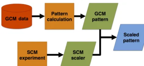
Pattern scaling was initially established to enable the cre-ation of transient climate projections from the steady state response of a GCM to a doubling of the preindustrial CO2 concentration (Santer et al., 1990). Under the assumption that a climate variable from a GCM scales proportionally with global mean temperature (GMT) change, patterns are derived from multiple GCMs. Those patterns can then be scaled in magnitude by a specified GMT change or by the GMT change obtained from a simple climate model (SCM) to span a wide range of future scenarios (Moss et al., 2010) that have not been simulated by full GCMs (Fig. 1).
Figure 1.Generalized flowchart of pattern scaling process.
method or the “delta” method, where local future change in a climate variable is normalized by future GMT change aver-aged over some chosen time period, hereafter referred to as anepoch(Osborn, 2009; Tebaldi and Arblaster, 2014; Herger et al., 2015). The second is the linear regression method, which uses ordinary least squares regression coefficients to fit local trends to a GMT time series (Mitchell, 2003; Ruos-teenoja et al., 2007; Lopez et al., 2013; Osborn et al., 2015). In terms of computational efficiency, the delta method is the fastest, which is a reason why it is predominantly used (Herger et al., 2015). However, in terms of skill in trend esti-mation and adaptability to additional predictors, the linear re-gression method is preferable (Mitchell, 2003; Frieler et al., 2012; Lustenberger et al., 2014; Barnes and Barnes, 2015).
In pattern scaling several broad assumptions are made. First, it is assumed that patterns generated under different forcing scenarios are not significantly different. Tebaldi and Arblaster (2014) found that patterns from different scenarios were highly spatially correlated, and that choice of scenario did not explain a significant proportion of variability in pat-terns when using the delta pattern scaling method. For the linear regression methodology, Mitchell (2003) found that the linear regression method reduces the influence of the non-linearities arising from differing rates of warming, but the magnitudes of estimation errors vary between scenarios and climate variables due to nonlinearity in GMT relationships.
Second, it is assumed that responses to external forcing and internal variability are independent, implying that an-thropogenic forcings do not modify the internal variability of the climate system (Mitchell, 2003; Lopez et al., 2013), but this premise is not always true (Screen, 2014). Changes in variability may introduce estimation errors in pattern fit; in practice, estimation errors introduced through this assump-tion at the global scale were small, although they can be large enough at the regional scale to mislead adaptation decisions (Lopez et al., 2013).
Third, it is assumed that local change scales proportionally with GMT change, and that the relationship is stationary over time (Mitchell, 2003). This assumption is not always true in the climate system, especially considering different forcing scenarios and spatial heterogeneity of projected change. For temperature variables, the assumption of stationarity is
gen-erally valid, but the magnitudes of estimation errors vary be-tween scenarios for non-temperature variables (Frieler et al., 2012) and temperature extremes on the upper tail of the tem-perature distribution (Lustenberger et al., 2014). Lopez et al. (2013) found that when pattern scaling temperature extremes over southern Europe, the magnitude of the error in the pat-tern estimates was large. In linear regression, the error term is assumed to have a normal distribution with a mean of zero. So it is likely that outliers or climate extremes would be in the very end of the tails and yield high error terms. This can be problematic when constructing confidence intervals but is not necessarily a limitation in the pattern scaling methodol-ogy, nor in the resulting patterns (Lustenberger et al., 2014). Currently there are three prominent online tools and soft-ware that generate climate patterns and scale them with spe-cific SCM scalers (Wigley, 2008; Osborn, 2009; Castruccio et al., 2014). These tools lock the user into using a specific SCM and do not provide pattern data and diagnostics, which can be important for understanding individual model scaled patterns. For uncertainty quantification and probabilistic sta-tistical analysis, a library of patterns with descriptive statis-tics for each file would be beneficial, but such a library does not presently exist.
Using a sub-selection of climate models, this paper first examines surface temperature patterns generated by the two primary pattern generation methods, and explores the dif-ferences in patterns across two forcing scenarios. We focus on spatial heterogeneity and magnitude of the local response to GMT change (hereafter called “pattern sensitivity”) from both pattern estimation methodologies. We then present a de-scription of our pattern library and code to generate the pat-terns.
2 Data/methods
2.1 Climate models
We employed three sets of experiments from the Coupled Model Intercomparison Project Phase 5 (CMIP5; Taylor et al., 2011). The “historical” experiment was used to con-struct reference epochs for use in pattern creation via the delta method. Model historical runs varied in length, so we used 1861 as the start of the historical period, and 2005 as the end. For future projections, we used the high-forcing rcp8.5 scenario, in which radiative forcing increases to 8.5 W m−2 through the 21st century (Riahi et al., 2011), and the mid-forcing rcp4.5 scenario, in which radiative mid-forcing increases to 4.5 W m−2 through the 21st century (Thomson et al., 2011) achieved by limiting future emissions. For the future simulations, the start year was 2006, and the end year was 2100.
chose not to average over multiple realizations from each model. This was done because some modeling centers only archived/produced one realization for each model–scenario combination, and the magnitude of the local response to GMT change across realizations is assumed to be consistent. For this study, only seasonal and annual surface air tem-perature was analyzed, and in some cases, the influence of the land–ocean contrast was examined. For such cases, a land mask was applied using each model’s native resolution, with 100 % of the grid cell either land or ocean. Assessment of patterns generated by each methodology was done by exam-ining the multi-model ensemble mean as well as the uncer-tainty represented by the model spread.
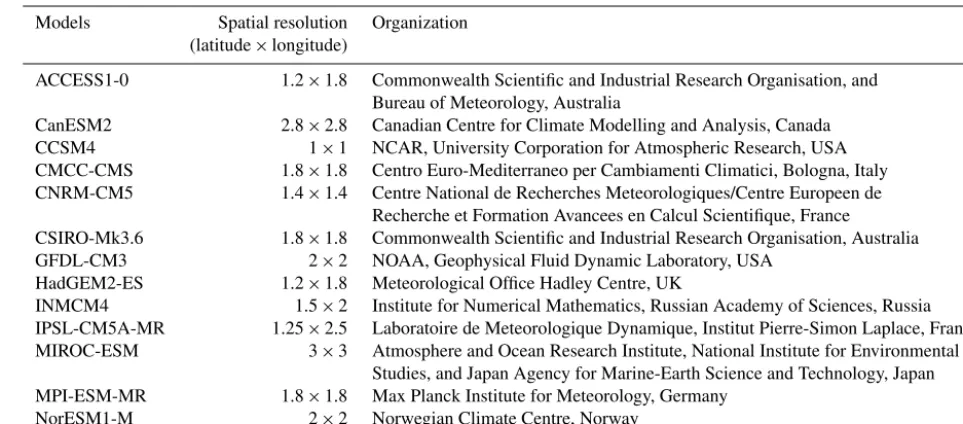
All model output was regridded to the lowest spatial res-olution of the multi-model ensemble prior to the calculation of an ensemble mean or median (Table 1). This was done for averaging purposes, as each model had a different spatial resolution. Regridding to the lowest resolution of the multi-model ensemble is a conservative assumption that avoids in-terpolation errors.
2.2 Data analysis
The delta pattern (DP) is described as follows:
DPMS=
1TLMS
1TGMS
. (1)
For each model (M) and future scenario (S), local (two-dimensional, a value for each latitude and longitude pair) temperature change (TL) is normalized by global (scalar value) mean temperature change (TG), with respect to a 30-year reference epoch from the CMIP5 historical simulation.
All epochs were 30 years in length, as it was assumed that the length of epochs used should not alter the result-ing pattern. Barnes and Barnes (2015) argue that the ideal epoch length is dependent on minimizing variable variance by selecting a epoch length with a high signal-to-noise ra-tio, which is largely dependent on length of time series, and whether the trend in the time series is linear. They found that for temperature, one-third the length of the time series is ideal, and for a 100-year time series (or longer) a 30-year epoch length is sufficient. Throughout the IPCC Fifth As-sessment Report (AR5; Stocker et al., 2013) a 20-year refer-ence epoch of 1986–2005 was used for discussion of pro-jected anomalies; previous assessment reports used earlier epochs. In impact studies, a later reference epoch is more suitable because it is more representative of the current cli-mate, and hence what socioeconomic systems were already somewhat adapted to (Fowler et al., 2007; Herger et al., 2015). In adaptation/mitigation analyses, a preindustrial con-trol simulation epoch is often used as the baseline from which change is diagnosed, as this period has little to no anthro-pogenic forcing. However, for pattern generation, an epoch in the later half of the 20th century is often used (Osborn, 2009; Tebaldi and Arblaster, 2014).
For the aforementioned epoch variations, we used two ref-erence epochs to generate patterns: a late 19th (1861–1890) and a late 20th (1971–2000) century average, hereafter re-ferred to as L19C and L20C, respectively. The bulk of the epoch patterns use a future epoch that spans the last 30 years of the 21st century (2071–2100), but a mid-21st century (2041–2070) epoch was also used when examining epoch pattern differences. These epochs were hereafter referred to as L21C and M21C, respectively, in the figures and text.
The least squares regression (LSR) patterns were calcu-lated from future forcing scenarios only. We use a least squares approach, which provides the best fit for calculating the regression pattern:
TLMS=αMS+βMS×TGMS+MS. (2)
In this equation, TG is the GMT time series (one-dimensional, unsmoothed), and TL is the gridded time series (three dimensional).β is a two-dimensional field of regres-sion slopes, andis a three-dimensional residual term (error) stemming from linearly fitting the dependent variable to the predictor.αis theyintercept, which we take to be 0 by only computing change, not absolute temperature.
To examine the assumption that the multi-model ensemble probability distribution and the sample mean between pat-terns and scenarios generated by each method were not sig-nificantly different, we calculated the Student’st-distribution probability. This was done because the ensemble consists of only 12 models, which poorly samples the space of possi-ble modeled climate realizations, and because we assume the ensemble variance for each pattern is the same. The resulting probability indicates where there is a significant difference between patterns generated by each method.
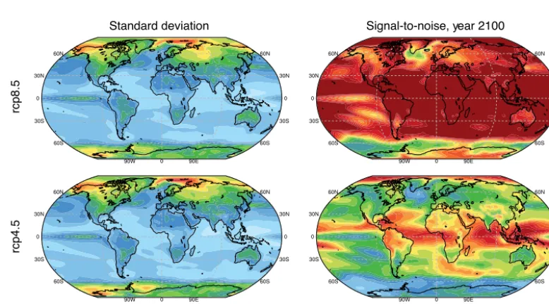
Pattern estimation can be skewed by local variability be-cause large variability can mask the local warming signal. To identify areas where pattern fit is poor due to high variabil-ity, we calculated the detrended 21st century variance and the signal-to-noise ratio as defined by Hawkins and Sutton (2012). The signal-to-noise ratio identifies regions where the magnitude of the warming signal in relation to historical vari-ability is large. The signal calculation in the signal-to-noise ratio makes an assumption that local temperature changes scale with global temperature (Hawkins and Sutton, 2012), similar to pattern scaling methodologies.
Table 1.List of the CMIP5 models and their respective spatial resolution and organization used in this analysis.
Models Spatial resolution Organization (latitude×longitude)
ACCESS1-0 1.2×1.8 Commonwealth Scientific and Industrial Research Organisation, and Bureau of Meteorology, Australia
CanESM2 2.8×2.8 Canadian Centre for Climate Modelling and Analysis, Canada CCSM4 1×1 NCAR, University Corporation for Atmospheric Research, USA CMCC-CMS 1.8×1.8 Centro Euro-Mediterraneo per Cambiamenti Climatici, Bologna, Italy CNRM-CM5 1.4×1.4 Centre National de Recherches Meteorologiques/Centre Europeen de
Recherche et Formation Avancees en Calcul Scientifique, France CSIRO-Mk3.6 1.8×1.8 Commonwealth Scientific and Industrial Research Organisation, Australia GFDL-CM3 2×2 NOAA, Geophysical Fluid Dynamic Laboratory, USA
HadGEM2-ES 1.2×1.8 Meteorological Office Hadley Centre, UK
INMCM4 1.5×2 Institute for Numerical Mathematics, Russian Academy of Sciences, Russia IPSL-CM5A-MR 1.25×2.5 Laboratoire de Meteorologique Dynamique, Institut Pierre-Simon Laplace, France MIROC-ESM 3×3 Atmosphere and Ocean Research Institute, National Institute for Environmental
Studies, and Japan Agency for Marine-Earth Science and Technology, Japan MPI-ESM-MR 1.8×1.8 Max Planck Institute for Meteorology, Germany
NorESM1-M 2×2 Norwegian Climate Centre, Norway
RMSE=
r P
x h
ˆ
B(x)−B(x)·A(x)i2
q P
x[A(x)]2
, (3)
whereA(x) is the area of the grid boxx and sums were cal-culated over allx.
3 Pattern results
3.1 Pattern differences
For the delta methodology, choice of epoch can be important. In our ensemble at the local spatial scale, absolute tempera-ture differences between reference epochs were small, but differences in future epochs often exceeded 2◦C in rcp8.5, particularly over land and at high latitudes (Fig. 2). Patterns across epochs were similar despite differences in the rate of GMT change and absolute temperature differences in epochs (Fig. 3). Differences between reference epoch patterns were largest in the Northern Hemisphere mid- and high latitudes, but differences were generally not significant, except for the Great Lakes region of North America in December through February (DJF) and over the North Pacific Basin and eastern Asia in June through July (JJA). These differences in patterns across reference epochs were amplified when the mid-21st century future epoch is used, as compared to the late 21st century future epoch.
Regardless of epoch chosen for the delta method, the resulting patterns were similar to the regression patterns (Fig. 4). The key idea in either pattern scaling method is that local temperature change scales with global tempera-ture change, despite different ways of calculating the local–
global relationship. With the exception of the high latitudes, the differences in the annual pattern were small (<0.2◦C). Pattern differences were similar across seasons, but differ-ences in patterns were the largest in DJF, particularly for the delta pattern with the earlier reference period. The regres-sion patterns have a stronger temperature sensitivity to GMT change in the Northern Hemisphere and a weaker tempera-ture sensitivity in the Southern Hemisphere at high latitudes as compared to the delta methods. These differences in sen-sitivity stem from how each methodology captures the effect of Arctic amplification, where the warming trend in the Arc-tic is almost twice as large as the trend in the global average, but the effect of Arctic amplification on pattern generation is not explored here.
There were few regions where the patterns differ signifi-cantly (Fig. 4), and there were fewer significant differences between the regression method and the delta method using the L20C epoch over the L19C epoch. Significant differences between patterns generated from each method were shown in the Baltic/northern European region for both epochs in the annual and DJF pattern, but in the earlier epoch, signifi-cant differences across seasons were shown in the northwest-ern Pacific region. In general, the temperature pattnorthwest-erns across methods were very similar.
AN
N
D
JF
JJA
L20C – L19C
rcp8.5 L21C – M21C
rcp4.5 L21C – M21C
oC
Figure 2.Ensemble mean temperature difference (◦C) between the L20C (1971–2000) and L19C (1861–1890) epoch; the L21C (2071– 2100) and M21C (2041–2070) epoch from the rcp8.5 scenario; and the L21C and M21C epoch from the rcp4.5 scenario for mean annual, DJF, and JJA.
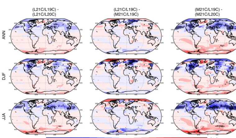
(L21C/L19C) -(L21C/L20C)
(L21C/L19C) -(M21C/L19C)
(M21C/L19C) -(M21C/L20C)
oC/ oC
AN
N
D
JF
JJA
Figure 3.Ensemble mean delta method pattern differences between L21C (2071–2100)/L19C (1861–1890) and L21C/L20C (1971–2000); L21C/L19C and M21C (2041–2070)/L19C; and M21C/L19C and M21C/ L20C for mean annual, DJF, and JJA using future forcing scenario rcp8.5. Significance values below the 95 % confidence interval using a Student’st-distribution probability statistic are stippled.
delta patterns have a strong temperature sensitivity over the Baltic/northern European region. Assuming that the GMT trend is linear, it appears that the regression pattern scaling method underestimates the relationship between global tem-perature and local temtem-perature when GMT change is 1◦C. However, the degree to which it overestimates the relation-ship is small (<0.08◦C).
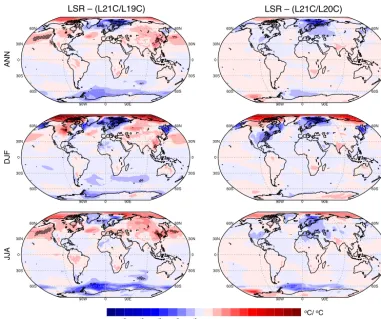
LSR – (L21C/L19C) LSR – (L21C/L20C)
AN
N
D
JF
JJA
oC/ oC
Figure 4.Ensemble mean regression method pattern and delta method pattern differences in ◦C/◦C for L21C (2071–2100)/L19C (1861– 1890) and L21C/L20C (1971–2000) for annual, DJF and JJA for future forcing scenario rcp8.5. Significance values below the 95 % confi-dence interval using a Student’st-distribution probability statistic are stippled.
Table 2.Root mean square difference between actual and pattern predicted global mean anomalies in◦C/◦C for each pattern method-ology at the end of the 21st century.
L21C/L19C L21C/L20C LSR Annual rcp8.5 0.156 0.110 0.039 rcp4.5 0.149 0.103 0.034 DJF rcp8.5 0.179 0.127 0.059 rcp4.5 0.173 0.120 0.050 JJA rcp8.5 0.136 0.095 0.034 rcp4.5 0.130 0.089 0.028
relationship between global and local temperature as seen in Fig. 6. Nevertheless, Table 2 indicates that the both method-ologies do well emulating actual model output.
Overall, the annual and seasonal patterns from each method were not significantly different from each other, re-gardless of reference epoch for the delta method. The dif-ferences were slightly larger when using an earlier reference epoch, but the regions where the ensemble differences were
significant (above the 95 % significance level) were small. Our small ensemble size (12 models with only one realiza-tion) may have contributed to the lack of significance in dif-ferences across epoch patterns, particularly when using para-metric tests like calculatingpvalues for the Student’st test. A more robust analysis would include multiple realizations from all available models.
3.2 Scenario differences
rcp8.5 rcp4.5
L21C/L19C
L21C/L20C
L
SR
oC/ oC
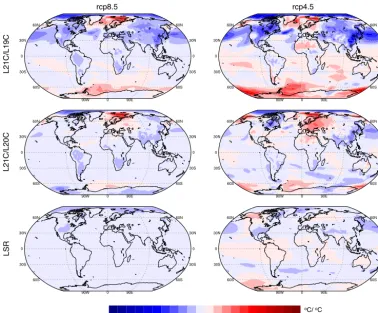
Figure 5.Difference between patterns predicted from L21C (2071–2100)/L19C (1861–1890), L21C/L20C (1971–2000), and LSR methods and annual multi-model mean change, when GMT change=1◦C for future forcing scenarios rcp8.5 and rcp4.5 in ◦C/◦C.
rcp4.5 scenario more difficult to estimate because the signal is harder to distinguish from the noise in this scenario.
Temperature change at high latitudes cannot be approxi-mated by a linear relationship due to strong regional feed-backs, for example Arctic amplification (Holland and Bitz, 2003), and therefore is not well predicted when using pat-tern scaling methods. The differences between scenarios are larger in the regression method, but both methods show similar spatial patterns. To further examine why the regres-sion method produces larger differences across scenarios, we looked at the linear fit of local temperature to GMT (Fig. 8). In the rcp8.5 scenario, the R2 values, between local tem-perature and GMT with respect to time, were large, but in the rcp4.5 scenario,R2values were much lower particularly along the Antarctic continent and in the North Atlantic. Even though the global/local fit is poorer in the rcp4.5 scenario, the lower forcing scenario predicted pattern is more like the actual model output (Table 2).
Large differences in patterns across scenarios were mainly due to a larger local / global ratio at high latitudes in the rcp4.5 scenario as compared to the rcp8.5 scenario (Fig. 9). These differences at high latitudes result from the nonlinear evolution of temperature due to retreating sea ice.
Sensitiv-ity of high latitudes to even small changes in GMT is evi-dent across scenarios, but the rcp4.5 scenario overestimates this relationship, resulting in substantial differences in pat-terns between the scenarios, particularly for the regression methodology.
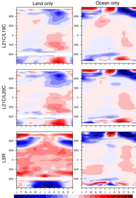
Differences between patterns across scenarios is further examined by separating the land and ocean patterns (Fig. 10). The differences between scenarios for the regression method when isolating the land/ocean pattern were comparatively large, especially over the Arctic and Antarctic regions. For the regression method, the rcp4.5 ocean-only pattern sensi-tivity is≥0.5◦C greater than the rcp8.5 (ocean only) tern sensitivity over the Arctic, and the rcp4.5 land-only pat-tern sensitivity is≥0.5◦C greater than the rcp8.5 (land only) pattern sensitivity over the Antarctic. The differences in pat-terns across scenarios for the delta method when isolating the land/ocean pattern were small except over the Arctic region, which shows strong seasonal differences (≥0.5◦C) in boreal autumn (SON). In this way the delta method is more consis-tent across future forcing scenarios, which should be taken into consideration when choosing methodology.
L
SR
L21C/L20C
L21C/L19C
rcp8.5 – rcp4.5 rcp8.5 / rcp4.5 p-value
oC/ oC
Figure 6.Ensemble annual average difference in ◦C/◦C and significance of difference using a Student’st-distribution probability statistic between future forcing scenarios rcp8.5 and rcp4.5 for L21C (2071–2100)/L19C (1861–1890), L21C/L20C (1971–2000), and LSR patterns.
rcp8.5
rcp4.5
Standard deviation Signal-to-noise, year 2100
oC
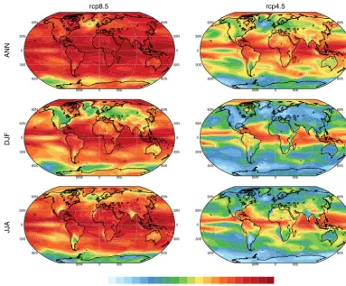
rcp8.5 rcp4.5
AN
N
D
JF
JJA
Figure 8.Ensemble mean of the square of the correlation coefficient between GMT and local surface temperature over the 21st century for rcp8.5 and rcp4.5 scenarios for annual mean, DJF, and JJA.
oC/ oC
Figure 9.Ensemble mean annual average difference in ◦C/◦C in the ratio of local / global linear trend over the 21st century (2006– 2100) between rcp8.5 and rcp4.5.
for scenarios with stronger mitigation (May, 2011; Ishizaki et al., 2012), even though we found that, for the models and scenarios we used, the lower forcing scenario patterns better emulated the actual model response. A weaker GMT signal coupled with nonlinear relationships between GMT change and local climate change (particularly in the Arctic) under
strong mitigation scenarios result in larger pattern errors. We found that differences in patterns between scenarios are more evident in the regression method as compared to the delta method, but similar features appear in the patterns produced by the delta method. How models incorporate sea ice may also add to the variability of patterns across models, but this is a subject we have not explored.
4 Code and data availability
CMIP5 model data are publicly available via the Earth System Grid Federation website (ESGF, https://pcmdi.llnl. gov/). Code used to construct this analysis is available on GitHub through the Joint Global Change Research Institution repository (https://github.com/JGCRI/CMIP5_ patterns/). Any additional data can be obtained from Cary Lynch ([email protected]).
5 Conclusions
Land only Ocean only
L
SR
L21C/L20C
L21C/L19C
oC/ oC
Figure 10. Ensemble mean temperature pattern differences in
◦C/◦C between rcp8.5 and rcp4.5 in zonal monthly means for land
only and ocean only for L21C (2071–2100)/L19C (1861–1890), L21C/L20C (1971–2000), and LSR patterns.
and with the assumption of linearity, the regression method-ology pattern outperforms the delta methodmethod-ology pattern. The regression methodology patterns also have lower RMSE, and better emulates actual model output. The simplistic de-sign of the regression method allows for additional pre-dictors (e.g., land/ocean term, latitudinal position, non-CO2 aerosols) in the pattern equation and confidence intervals to be easily calculated. The delta method introduces complexity in choice of reference epoch and length of reference epoch, but we have found little difference between patterns across epochs.
Choice of scenario can affect the resulting pattern, particu-larly at high latitudes. With the regression methodology pat-tern, the GMT temperature sensitivity is stronger when using the rcp4.5 scenario because the GMT trend is proportionally smaller and changes in GMT have a stronger effect on local temperature, particularly when strong mitigation is employed later in the simulation. Delta method patterns were more con-sistent across scenarios with less heterogeneity in local
tem-poral and spatial GMT sensitivity. With the assumption that different future forcing scenarios should not change the re-sulting pattern, the delta pattern is more consistent across scenarios, regardless of epoch chosen, despite differences in epoch means being large.
Our pattern library was created because the online tools and software that generates pattern scaling products do not provide pattern data and diagnostics, and do not offer flexi-bility in use of a SCM for scaling. Based on our analysis, we have created a library of patterns using the least squares re-gression methodology. We also provide descriptive statistics for each output file, which we believe to be beneficial for un-certainty quantification and probabilistic statistical analysis.
While this paper did not analyze precipitation, precipi-tation patterns are included in the library. The relationship between global mean temperature and local precipitation is complex and requires a more in-depth examination of pattern scaling methodologies and the resulting patterns. Therefore, we have written an entirely separate paper which discusses precipitation patterns (Kravitz et al., 2016).
Creation of a pattern library is the first step in our goal of exploring inter-model and future forcing uncertainty in cli-mate projections. Our next steps will be to push the current boundaries of pattern scaling by exploring scaling measures of climate variability and scaling of different variables, such as pH. Our efforts will be documented in future papers, and all patterns will be added to the repository.
6 Pattern library
The pattern library is available on GitHub through the Joint Global Change Research Institution repository (https://github.com/JGCRI/CMIP5-patterns). GitHub is a web-based version control repository and Internet hosting service which uses git concepts and commands. The purpose of creating this pattern library was to allow for researchers across various fields to be able to efficiently use the statistical patterns generated by the described regression method to ex-amine model response to change in global mean temperature for all the available CMIP5 models (41 models, at present). We also further intend for those patterns to be easy to scale using a scaler generated from a SCM of ones choosing.
The pattern library contains patterns, generated by the least squares regression methodology, for the first realiza-tion of the 41 CMIP5 climate models. Annual, seasonal, and monthly patterns are provided for surface temperature and precipitation. For temperature patterns, units in degrees Cel-sius were used as this is the standard temperature unit for impact analysis.
The following are included in each netCDF file for each model:
2. the adjustedR2 between the predictor and dependent terms (2-D);
3. the standard error of the estimated regression coefficient (2-D);
4. a historical climatology based on the 1961–1990 average from each model (2-D), which can be used to construct absolute values at timeX;
5. the 95th percentile confidence level pattern for model parameters.
The patterns from all 41 CMIP5 models range in size (165 kB to 1 MB) due to spatial resolution, but all patterns were kept at the native resolution of the dependent variable and no re-gridding of input/output variables was done. This was done to retain model specific information, which may have been lost if regridded to a common spatial resolution.
All source code used to produce patterns is available in the aforementioned repository. Source code is written in NCAR Command Language (version 6.3.0; http://dx.doi.org/ 10.5065/D6WD3XH5).
The Supplement related to this article is available online at doi:10.5194/essd-9-281-2017-supplement.
Competing interests. The authors declare that they have no con-flict of interest.
Acknowledgements. This research is based on work supported by the US Department of Energy, Office of Science, Integrated Assessment Research Program. The Pacific Northwest National Laboratory is operated for DOE by Battelle Memorial Institute under contract DE-AC05-76RL01830.
Edited by: M. E. Contadakis
Reviewed by: two anonymous referees
References
Barnes, E. A. and Barnes, R. J.: Estimating Linear Trends: Sim-ple Linear Regression versus Epoch Differences, J. Climate, 28, 9969–9976, doi:10.1175/JCLI-D-15-0032.1, 2015.
Castruccio, S., McInerney, D. J., Stein, M. L., Liu Crouch, F., Jacob, R. L., and Moyer, E. J.: Statistical Emulation of Climate Model Projections Based on Precomputed GCM Runs, J. Climate, 27, 1829–1844, doi:10.1175/JCLI-D-13-00099.1, 2014.
Christensen, J., Hewitson, B., Busuioc, A., Chen, A., Gao, X., Held, I., Jones, R., Kolli, R., Kwon, W.-T., Laprise, R., Rueda, V. M., Mearns, L., Menéndez, C., Räisänen, J., Rinke, A., Sarr, A., and
Whetton, P.: Regional Climate Projections, in: Climate Change 2007: The Physical Science Basis. Contribution of Working Group I to the Fourth Assessment Report of the Intergovernmen-tal Panel on Climate Change, edited by: Solomon, S., Qin, D., Manning, M., Chen, Z., Marquis, M., Averyt, K., Tignor, M., and Miller, H., chap. 11, Cambridge University Press, Cambridge, United Kingdom and New York, NY, USA., 2007.
Dessai, S., Lu, X., and Hulme, M.: Limited sensitivity analysis of regional climate change probabilities for the 21st Century, J. Geophys. Res.-Atmos., 110, D19, doi:10.1029/2005JD005919, 2005.
Fowler, H. J., Blenkinsop, S., and Tebaldi, C.: Linking climate change modelling to impacts studies: recent advances in down-scaling techniques for hydrological modelling, Int. J. Climatol., 27, 1547–1578, doi:10.1002/joc.1556, 2007.
Frieler, K., Meinshausen, M., Mengel, M., Braun, N., and Hare, W.: A Scaling Approach to Probabilistic Assessment of Regional Cli-mate Change, J. CliCli-mate, 25, 3117–3144, doi:10.1175/JCLI-D-11-00199.1, 2012.
Hawkins, E. and Sutton, R.: Time of emergence of climate signals, Geophys. Res. Lett., 39, L01702, doi:10.1029/2011GL050087, 2012.
Herger, N., Sanderson, B. M., and Knutti, R.: Improved pattern scal-ing approaches for the use in climate impact studies, Geophys. Res. Lett., 42, 3486–3494, doi:10.1002/2015GL063569, 2015. Holland, M. M. and Bitz, C. M.: Polar amplification of
cli-mate change in coupled models, Clim. Dynam., 21, 221–232, doi:10.1007/s00382-003-0332-6, 2003.
Ishizaki, Y., Shiogama, H., Emori, S., Yokohata, T., Nozawa, T., Ogura, T., Abe, M., Yoshimori, M., and Takahashi, K.: Temper-ature scaling pattern dependence on representative concentration pathway emission scenarios, Climatic Change, 112, 535–546, doi:10.1007/s10584-012-0430-8, 2012.
Kravitz, B., Lynch, C., Hartin, C., and Bond-Lamberty, B.: Ex-ploring precipitation pattern scaling methodologies and robust-ness among CMIP5 models, Geosci. Model Dev. Discuss., doi:10.5194/gmd-2016-258, in review, 2016.
Lopez, A., Suckling, E. B., and Smith, L. A.: Robustness of pattern scaled climate change scenarios for adaptation decision support, Climatic Change, 122, 555–566, doi:10.1007/s10584-013-1022-y, 2013.
Lustenberger, A., Knutti, R., and Fischer, E. M.: The potential of pattern scaling for projecting temperature-related extreme in-dices, Int. J. Climatol., 34, 18–26, doi:10.1002/joc.3659, 2014. May, W.: Assessing the strength of regional changes in near-surface
climate associated with a global warming of 2◦C, Climatic Change, 110, 619–644, doi:10.1007/s10584-011-0076-y, 2011. Mitchell, T. D.: Pattern Scaling: An Examination of the Accuracy of
the Technique for Describing Future Climates, Climatic Change, 60, 217–242, doi:10.1023/A:1026035305597, 2003.
Moss, R., Edmonds, J., Hibbard, K., Manning, M., Rose, S., van Vuuren, D., Carter, T., Emori, S., Kainuma, M., Kram, T., Meehl, G., Mitchell, J., Nakicenovic, N., Riahi, K., Smith, S., Stouffer, R., Thomson, A., Weyant, J., and Wilbanks, T.: The next gener-ation of scenarios for climate change research and assessment, Nature, 463, 747–756, doi:10.1038/nature08823, 2010. Osborn, T.: A user guide for ClimGen: a flexible tool for
available at: https://crudata.uea.ac.uk/~timo/climgen/ClimGen_ v1-02_userguide_2feb2009.pdf, 2009.
Osborn, T. J., Wallace, C. J., Harris, I. C., and Melvin, T. M.: Pattern scaling using ClimGen: monthly-resolution future climate sce-narios including changes in the variability of precipitation, Cli-matic Change, 134, 353–369, doi:10.1007/s10584-015-1509-9, 2015.
Riahi, K., Rao, S., Krey, V., Cho, C., Chirkov, V., Fischer, G., Kin-dermann, G., Nakicenovic, N., and Rafaj, P.: RCP 8.5 – A sce-nario of comparatively high greenhouse gas emissions, Climatic Change, 109, 33–57, doi:10.1007/s10584-011-0149-y, 2011. Ruosteenoja, K., Tuomenvirta, H., and Jylhä, K.:
GCM-based regional temperature and precipitation change estimates for Europe under four SRES scenarios applying a super-ensemble pattern-scaling method, Climatic Change, 81, 193– 208, doi:10.1007/s10584-006-9222-3, 2007.
Santer, B., Wigley, T., Schlesinger, M., and Mitchell, J.: Developing Climate Scenarios from Equilibrium GCM Results, Tech. rep., Hamburg, Germany, 1990.
Screen, J. A.: Arctic amplification decreases temperature variance in northern mid- to high-latitudes, Nature Climate Change, 4, 577–582, 2014.
Stocker, T., Qin, D., Plattner, G.-K., Tignor, M., Allen, S., Boschung, J., Nauels, A., Xia, Y., Bex, V., and Midgley, P. (Eds.): IPCC, 2013: Climate Change 2013: The Physical Science Basis. Contribution of Working Group I to the Fifth Assessment Report of the Intergovernmental Panel on Climate Change, Cambridge University Press, Cambridge, United Kingdom and New York, NY, USA, 1535 pp., doi:10.1017/CBO9781107415324, 2013. Taylor, K. E., Stouffer, R. J., and Meehl, G. A.: An Overview of
CMIP5 and the Experiment Design, B. Am. Meteorol. Soc., 93, 485–498, doi:10.1175/BAMS-D-11-00094.1, 2011.
Tebaldi, C. and Arblaster, J. M.: Pattern scaling: Its strengths and limitations, and an update on the latest model simulations, Cli-matic Change, 2014.
Thomson, A. M., Calvin, K. V., Smith, S. J., Kyle, G. P., Volke, A., Patel, P., Delgado-Arias, S., Bond-Lamberty, B., Wise, M. A., Clarke, L. E., and Edmonds, J. A.: RCP4.5: a pathway for sta-bilization of radiative forcing by 2100, Climatic Change, 109, 77–94, doi:10.1007/s10584-011-0151-4, 2011.