Optimal Use of Put Options in a Stock
Portfolio
Bell, Peter N
University of Victoria
13 March 2014
© Peter Bell, 2014
Optimal Use of Put Options in a Stock Portfolio
Peter N. Bell
Department of Economics, University of Victoria
March 29, 2014
This research was supported by the Joseph-Armand Bombardier Canada Graduate Scholarship –
Doctoral through the Social Sciences and Humanities Research Council from the Government of
Abstract
I analyze a portfolio optimization problem where an agent holds an endowment of stock and is
allowed to buy some quantity of a put option on the stock. My model rephrases a fundamental
question from insurance economics: how much coverage should a risk averse agent buy? Classic
studies of rational insurance purchasing use exact algebraic analysis with a binomial probability
model of portfolio value to explore this problem. In contrast, I use numerical techniques to
approximate the probability distributions for key variables. Using large-sample, asymptotic
analysis, I identify the optimal quantity of put options for three types of preferences over the
distribution of portfolio value. The location of the optimal quantity varies with preferences and
provides examples of important concepts from the rational insurance purchasing literature:
coinsurance for log utility (q*<1), full-insurance for quantile-based preferences (q*=1), and
over-insurance for mean-variance utility (q*>1). I use resampling analysis to show that the
optimal quantity is well defined for mean-variance and quantile-based preferences, but the
optimal quantity for log utility is not stable. Although my analysis corroborates the classic result
that coinsurance is optimal for log utility, I show that the specific amount of coinsurance is not
well defined. In addition, the optimal quantity for mean-variance utility in my model is not
allowed in a classic insurance model. By matching and extending the set of results for basic
rational insurance purchasing, my research demonstrates the value of using numerical techniques
to analyze the optimal use of financial derivatives in a continuous setting.
Keywords: Portfolio optimization, financial derivative, put option, quantity, expected
Optimal Use of Put Options in a Stock Portfolio
Introduction
In this working paper I explore how to use financial derivatives. I present a portfolio
optimization problem where an agent holds one unit of stock and is allowed to buy a put option
on the stock. What quantity of put options should he buy? Although this question receives brief
attention from Philip Jorion in terms of the minimum variance hedge ratio (2007, p. 296), I frame
my research in context of a topic in insurance economics: rational choice of insurance coverage.
The classic approach to rational insurance purchasing uses an exact, analytic solution to the
portfolio optimization problem (Mossin, 1968). I update this approach with modern perspectives
on financial derivatives and numerical analysis.
Jan Mossin is an influential scholar in the economic theory of risk taking. His 1968
article provides the phrase rational insurance purchasing to describe the analysis of insurance
from the buyer’s perspective. The article attempts to “illustrate the power of the expected utility
approach to problems of risk taking” (1968, p. 553) by exploring three questions: the maximum
premium an agent would pay to buy insurance, the optimal amount of insurance coverage at a
given premium, and the optimal deductible amount. I focus on Mossin’s contribution to this
second question, the optimal amount of insurance coverage, because it can be rephrased today as:
how best to use financial derivatives to mitigate the risk of loss.
Mossin separates wealth into several different terms (safe wealth, risky wealth, and size
of loss). Although this definition of wealth requires cumbersome notation, given in Equation (1),
it produces a parsimonious model for optimal coverage (1968, p. 557). Mossin uses the model to
generate testable implications about risk aversion based on insurance choices (1968, p. 564).
(1) Y = A + L – X + (C/L)X – p C
The key variable in Mossin’s model is total wealth or portfolio value (Y). The other
variables are defined as follows: safe wealth (A), risky wealth (L), size of loss (X), price of
insurance (p), and amount of coverage for loss (C). Since the size of loss (X) is the only random
the net payoff for a financial derivative ((C/L)X – p C). This separation of total value into two
terms is a simple and powerful idea that I will use in my model.
The objective in Mossin’s model is to maximize expected utility over wealth (E(U(Y))). The agent’s choice variable is the level of coverage (C), which is constrained because an agent cannot buy more coverage than the value of the asset (0≤C≤L). Mossin solves the optimization
problem algebraically. He shows that the first order conditions evaluated at the boundaries for
the choice variable (C=0 or L) justify an interior solution (1968, p. 557), but he is not able to
produce an exact formula for the solution in general.
To gain analytic traction, Mossin specifies a model that yields an analytic solution (log
utility and binomial probability model for loss). He uses comparative statics to show how the
optimal coverage changes with wealth, which provides the foundation for the testable predictions
mentioned above (1968, p. 558). The binomial model that Mossin uses is a classic part of
insurance economics because it characterizes a situation where the agent suffers either no loss or
the complete loss of an asset. The binomial model provides an exact solution, which is valuable
in modern mathematical economics, but the results are limited because they only consider losses
of one size.
Mossin’s 1968 article was influential. It was extended by Razin (1976) to consider the minimax regret function from Leonard Savage’s decision theory and again by Briys & Loubergé
(1985) to consider bounded rationality, an important extension to rational choice theory. Since
both subsequent articles extended Mossin’s model by changing the objective function, I use three
types of preferences in my model. I use the familiar log and mean-variance utility functions, and
a based objective function inspired by Value at Risk (VaR). Although the
quantile-based objective is not a utility function, it is relevant to risk management decisions.
Both Razin (1976) and Briys & Loubergé (1985) kept the binomial probability model that
Mossin introduced. My model maintains the basic structure of wealth as a random asset plus a
financial derivative, but I abandon the binomial model. Instead, I focus on numerical analysis of
continuous probability models. I specify an interval of values for the choice variable, simulate
the distribution of wealth for each value as a statistical ensemble, and then compare the
Model Setup
To develop my model, I briefly discuss assumptions about the agent and his portfolio. I
assume that the agent cares only about the portfolio value when the derivative expires, as in
Mossin (1968). The portfolio value at expiry is random, but the agent knows the probability
distribution for the value. The agent also knows how the derivative affects the distribution of
portfolio value; thus, he can rank different quantities of put options. This model is classic
decision theory: portfolio optimization with perfect information.
I assume the portfolio is composed of one unit of stock and some quantity of European
put options. The agent knows the initial value of the stock and the distribution of the future
value. The put option is infinitely divisible, the strike price is equal to the initial stock price (at
the money), and the stock expires in one time step (one year). Equation (2) represents the agent’s portfolio optimization problem in this simple setting.
(2) max q>0 V(W(q)) s.t. W(q) = S + N(S,q)
The choice variable in Equation (2) is the quantity of derivatives (q). The objective
function is denoted as V(), which can be thought of as expected utility. For robustness, I use
three different forms for V(). The forms represent important preferences in the literature
(expected log utility, mean-variance utility1, and 5% quantile2). The value of the portfolio at
expiry is denoted W(q), which is a random variable. The value of the stock at expiry is denoted
as S and net payoff for the derivative is N(S,q).
(3) N(S,q) = q [ (K-S)+ - O ]
Equation (3) defines the net payoff for a put option. The quantity (q) appears as a linear,
multiplicative term. The term (K-S)+ is the intrinsic value of the put at expiry. As above, I
assume the strike (K) is equal to the stock price when the agent makes the initial decision for the
quantity (q). I calculate the option price (O) using the Black-Scholes formula because the stock
price is log-normal. When the agent picks q, they do not know the net payoff of the put option
because the value of N(S,q) depends on the future value of the stock (S), which is random.
1 I use a standard value for the risk aversion coefficient (λ=0.1) for the mean-variance utility (U(X)=µ-(λ/2)σ2). 2 Defined by the distribution of portfolio value (W(q)). It is w such that: Pr(W(q)<w)=0.05. Note that VaR is the
Numerical Analysis
In the numerical analysis of my model, I assume specific values for all parameters. For
example, I assume that the initial price of the stock is $100 and the returns are normally
distributed with 0% average and 10% volatility for one time step. This model for asset value
satisfies the random walk hypothesis and provides a basis for pricing the put option with
Black-Scholes. I provide further details on these assumptions in an appendix, which contains Matlab
code that can reproduce all of my results.
Asymptotic Analysis
For each value of q in an interval ([0.00,2.00] with step size 0.01), I simulate the stock
price a large number of times (1,000,000) to estimate the distribution of portfolio value for that
quantity. I calculate utility over the distribution and analyze it in several different ways. To
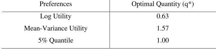
[image:7.612.119.490.376.460.2]begin, I report the optimal quantity (q*) for each type of preferences in Table 1.
Table 1: Optimal quantity of put options for different preferences
Preferences Optimal Quantity (q*)
Log Utility 0.63
Mean-Variance Utility 1.57
5% Quantile 1.00
Table 1 shows that the optimal quantity differs across the three preferences. The standard
question for the insurance literature is whether it is better to have full insurance (q*=1) or
coinsurance (q*<1) and Table 1 shows that both are optimal under different preferences in my
model. As in prior research, the optimal choice for log utility is coinsurance (q*=0.63).
However, the optimal choice for quantile-based preferences is and full insurance (q*=1.00),
which is a striking result in a numerical setting because it is on a knife-edge. Table 1 also shows
that the optimal quantity for mean-variance utility is well above one (q*>1), which is
inadmissible in the classical model of rational insurance purchasing. Table 1 suggest that my
modelling framework can generate results that match and extend the classic results from a
Now that I have identified the optimal choice across different preferences, I briefly
characterize each optimum. I do this by estimating the shape of the objective function over a
range of values for the choice variable. This is straightforward because the objective function
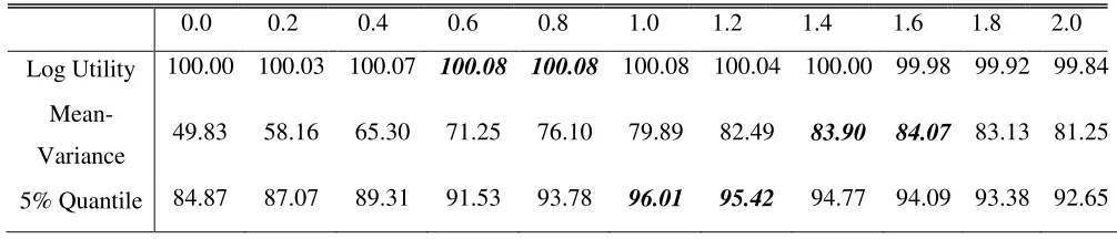
and choice variable are each 1-dimensional in my model. In Table 2 I report a money-metric
associated with the expected utility for each value of the choice variable and utility measure. For
the log and mean-variance utility, this money-metric is the certainty equivalent. For the
quantile-based objective function, the money-metric is the 5% quantile from the distribution of portfolio
[image:8.612.52.555.263.371.2]value. For each type of preference, a higher value is preferred to a lower value.
Table 2: Shape of objective function for range of values for choice variable
0.0 0.2 0.4 0.6 0.8 1.0 1.2 1.4 1.6 1.8 2.0
Log Utility 100.00 100.03 100.07 100.08 100.08 100.08 100.04 100.00 99.98 99.92 99.84
Mean-
Variance 49.83 58.16 65.30 71.25 76.10 79.89 82.49
83.90 84.07 83.13 81.25
5% Quantile 84.87 87.07 89.31 91.53 93.78 96.01 95.42 94.77 94.09 93.38 92.65
Table 2 provides a basic sense of the shape of the objective function using a sparse
sampling rate for the choice variable (0.2 units apart). I highlight two data points around the
optimal quantity for each type of preferences in bold and italics. Table 2 shows that the optimal
quantities for the mean-variance utility and the quantile-based objective functions are both
well-defined because the objective functions are concave around the optimums. In contrast, the
results for the log utility raise concerns because there is little variation in the agent’s valuation of
different portfolios. The results suggest that optimal quantity for log utility may not be robust to
sample selection. Although Table 2 uses sparse sampling points, the results give confidence in
optimum under the mean-variance utility and the 5% quantile preferences, but not the log utility.
When an agent with mean-variance utility holds zero put options (q=0), Table 2 shows
that he would trade the portfolio for $50. Note that the initial value of the stock is $100. The
large difference between valuations speaks to the negative effect of risk on a risk-averse agent.
If the same agent buys a close approximation to his optimal quantity of put options (q*=1.6),
then he would be much better off and would trade the portfolio for $84.07. This significant
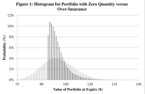
Figure 1 shows how a put option changes the probability distribution of portfolio value.
The figure shows a discrete approximation for the continuous density function. The shape
marked by light bars represents the portfolio with zero put options and the shape marked by dark
bars represent the portfolio with over-insurance. When an agent decides what quantity of put
option to buy, he is effectively picking which distributions he likes best. As such, visualizing
these distributions can tell us a lot about how preferences are driving decisions.
There are two important features in Figure 1. First, the probability of low values for the
portfolio is less when the agent buys put options; this is because put options are designed to
offset losses. Notice how the value of the portfolio with derivatives is never less than $90.
Second, the probability of high values for the portfolio is also less when the agent buys put
options; this is because the agent has to pay for the put options in the good times. Notice how
the right tail is lower when the agent buys the option. These two features show that
over-insurance reduces the frequency and severity of both high and low values for the portfolio, which
reduces the variance of the portfolio value at both ends and benefits a risk-averse agent. 0%
2% 4% 6% 8% 10% 12%
75 90 105 120 135 150
P
rob
ab
il
ity
(%
)
[image:9.612.74.541.207.511.2]Value of Portfolio at Expiry ($)
Figure 1: Histogram for Portfolio with Zero Quantity versus
Over-Insurance
Robustness to Small Sample
The analysis so far uses a single, large sample to establish all results. This asymptotic
analysis may hide variability that develops as the sample changes. To detect such variability I
conduct further simulations with resampling. Basically, I repeat the analysis above to estimate
the distribution for the optimal value, but I use a smaller sample size (1,000 draws of S) and loop
the calculation many times (10,000 estimates of q*). I present the distribution of the optimal
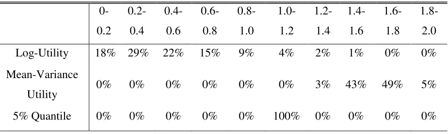
[image:10.612.77.539.256.395.2]values in Table 3.
Table 3: Frequency for location of optimal quantity (q*) by preferences
0-0.2 0.2-0.4 0.4-0.6 0.6-0.8 0.8-1.0 1.0- 1.2 1.2-1.4 1.4-1.6 1.6-1.8 1.8-2.0
Log-Utility 18% 29% 22% 15% 9% 4% 2% 1% 0% 0%
Mean-Variance
Utility 0% 0% 0% 0% 0% 0% 3% 43% 49% 5%
5% Quantile 0% 0% 0% 0% 0% 100% 0% 0% 0% 0%
Table 3 shows the distribution of the optimal quantity across each objective function.
The columns in Table 3 are closed on the lower side and open on the upper side (0-0.2 denotes
the interval [0,0.2]). Table 3 shows that the distribution of the optimal value varies greatly by
preferences. Again, the results for the quantile-based preferences are striking because the
optimum is always located at the special point of full insurance (q*=1.00 with 100% frequency).
The results for the mean-variance utility are encouraging because they show a symmetric, narrow
distribution around the optimal value. Thus, the optimal quantity for the quantile-based and
mean-variance preferences are, in some sense, well behaved.
Table 3 shows the optimal quantity for log utility is not well behaved. The optimal
quantity is broadly dispersed between 0 and 1, indicating that the optimal quantity for log utility
is not robust to sample selection. This echoes the potential problem I noted in Table 2 for log
utility. A classic result from Mossin is that coinsurance is optimal for log utility (1968, p. 558).
My analysis shows that coinsurance is generally the optimal choice for log utility, but not
Conclusion
This paper analyzes a portfolio optimization problem where an agent holds one unit of
stock and is allowed to buy put options on the stock. This is a specific example of the general
situation where an agent endowed with an asset is allowed to trade derivatives on the asset. I
position this research in relation to the question of optimal coverage in the literature on rational
insurance purchasing. The rational insurance purchasing literature uses algebraic analysis to
identify an exact solution under a binomial probability model for asset values (Mossin, 1968). In
contrast, I use numerical analysis to approximate a solution under a log-normal probability
model. This different analytic perspective allows me to develop rich insight into the
optimization problem by approximating continuous variables of interest.
The results show that the character of the optimal quantity depends on the agent’s
preferences. I find it is always optimal to have full insurance for quantile-based preferences,
which is a striking numerical result that deserves further attention because the quantile-based
preferences are designed after the VaR risk measure. As in the classic insurance literature, I find
it is generally optimal to have coinsurance under log utility. However, I find the specific amount
of coinsurance is not robust to resampling. Sometimes the optimal quantity is greater than one,
which means over-insurance is optimal under log utility. These results reflect problems with log
utility that are related to issues raised by Ole Peters (2011).
The rational insurance purchasing literature explicitly disallows over-insurance (Mossin,
1968, p. 557). In contrast, my results show that over-insurance is the optimal choice for the
mean-variance utility function. To show how over-insurance affects an agent, I compare the
probability distribution of portfolio value for zero insurance against over-insurance. I find that,
in bad times, over-insurance decreases the severity and frequency of low values for the portfolio
because the agent receives the option payoff. In good times, over-insurance decreases the
severity and frequency of high values for the portfolio because the agent pays the option
premium. Thus, over-insurance reduces the frequency and severity for both high and low values
of the portfolio, which reduces the variance and benefits a risk-averse agent. My analysis
demonstrates that numerical techniques are valuable in this setting because they allow us to
identify optimal values with continuous probability models and continuous choice variables,
There are, of course, some limitations to my research. By using numerical techniques, I
have picked arbitrary values for many parameters and it is possible that different values for
parameters may change the qualitative nature of the results. Interested readers could investigate
the parameters in the stock price, the level of risk aversion, or the percentile used in the
quantile-based preferences. Another limitation is my simple assumptions about the agent’s portfolio. It is
possible that different values for the strike price of the option or the timing of cash flows could
change the results further. The model also takes a simple view of randomness; I use known
randomness, not Knightian uncertainty. It may be possible to extend the analysis to a Bayesian
setting with subjective beliefs about probability distributions and preferences, which may be a
useful guide for design of experiments with human subjects. Finally, all of my analysis has used
ensemble averages and the results may be very different with time averages; Ole Peters (2011)
has shown that time averages resolve misconceptions at the heart of expected utility theory
References
Briys, E.P., & Loubergé, H. (1985). On the Theory of Rational Insurance Purchasing: A Note.
The Journal of Finance, 40(2), 577-581.
Jorion, P. (2007). Financial Risk Manager (4th ed.). Hoboken, NJ: John Wiley and Sons Inc.
Mossin, J. (1968). Aspects of Rational Insurance Purchasing. Journal of Political Economy,
76(4), 553-568.
Peters, O. (2011). The time resolution of the St. Petersburg paradox. Philosophical Transactions
of the Royal Society A: Mathematical, Physical and Engineering Sciences, 369(1956).
4913-4931.
Appendix
%% Code Appendix -- Optimal Use of Derivatives % © Peter Bell, March 10 2014
% Written for Matlab to produce all results used in working paper. %
%% Section 1: Global Parameters % Set random number generator
clear all
stream = RandStream('mt19937ar','Seed',12);
RandStream.setDefaultStream(stream);
% Simulate price for stock
numPrice = 10^6; S0 = 100; sigma=0.1;
% Simulate option price
K = 100; r = 0;
d1 = (1/sigma)*(log(S0/K)+r+sigma^2/2); d2 = d1 - sigma;
O = cdf('norm',-d2,0,1)*K - cdf('norm',-d1,0,1)*S0;
% Agent Utility
lambda = 0.5; %
% Simulations in Section 3 for Asymptotic Setting
numSimOne = 201; qScaleOne=100; qStep=1/qScaleOne; resultTable = zeros(3,numSimOne);
% numSimOne represents # points for choice variable
% qScaleOne is parameter to make so that consider q in [0,2] % Each simulation has length numPrice (10^6), specified above
% Simulations in Section 4 for small samples
numSimTwo= 10^4; numPriceSmall = 1000;
% numSimTwo represents # of times that identify optimal quantity (q*) % numPriceSmall is length of time series, which replaces numPrice
%% Section 2: Demo with single value for choice variable % Goal: demonstrate how particular quantity affects utility
q = 0.5;
S = S0*exp(randn(numPrice,1)*sigma); W = S + q*(max(K-S,0)-O);
% Log Utility
exp(mean(log(S))) exp(mean(log(W)))
% Mean-Variance Utility
mean(S) - lambda*var(S) mean(W) - lambda*var(W)
% 5% Quantile for distribution
temp1(length(temp1)*5/100) temp2 = sort(W);
temp2(length(temp1)*5/100)
%% Section 3: Analyze shape of objective function in asymptotic setting % Goal: Calculate material for Table 1, 2, and Figure 1.
%
for numChoice = 1:numSimOne
qLoop = (numChoice-1)/qScaleOne
% Simulate large number of prices for each q, calculate objective
S = zeros(1,1); W = zeros(1,1); S = S0*exp(randn(numPrice,1)*sigma); W = S + qLoop*(max(K-S,0)-O);
% Log Utility
resultTable(1,numChoice) = exp(mean(log(W)));
% Mean-Variance Utility
resultTable(2,numChoice) = mean(W) - lambda*var(W);
% 5% Quantile for distribution
temp2 = sort(W);
resultTable(3,numChoice) = temp2(length(temp2)*5/100); resultTable(4,numChoice) = qLoop;
end
% Table 1:
qTemp = 1:20:220;
tableOne = [(qTemp-1)*qStep;resultTable(1:3, qTemp)];
% Table 2: Optimal Choice by Utility
[uMaxLog iMaxLog] = max(resultTable(1,:));
[uMaxMeanVar iMaxMeanVar] = max(resultTable(2,:)); [uMaxQuantile iMaxQuantile] = max(resultTable(3,:));
qStarLog = (iMaxLog-1)*qStep;
qStarMeanVar = (iMaxMeanVar-1)*qStep; qStarQuantile = (iMaxQuantile-1)*qStep;
tableTwo = [qStarLog qStarMeanVar qStarQuantile ]
% Figure 1: Calculate histogram for wealth with optimal derivative
WStarLog = S + qStarLog*(max(K-S,0)-O);
WStarMeanVar = S + qStarMeanVar*(max(K-S,0)-O);
histIndex = 75:1:150;
[nZeroPut xOutOne] = hist(S, histIndex);
[nOptimalPut xOutTwo] = hist(WStarMeanVar, histIndex);
figureOne = [xOutOne' (nZeroPut./numPrice)' (nOptimalPut./numPrice)'];
% Goal: Build Table 3 in paper (histogram of q* for each utility) %
for simCount = 1:numSimTwo
simCount
resultTable = zeros(3,numSimOne);
for numChoice = 1:numSimOne
qLoop = (numChoice-1)/qScaleOne;
S = S0*exp(randn(numPriceSmall,1)*sigma); W = S + qLoop*(max(K-S,0)-O);
% Log Utility
resultTable(1,numChoice) = exp(mean(log(W)));
% Mean-Variance Utility
resultTable(2,numChoice) = mean(W) - lambda*var(W);
% 5% Quantile for distribution
temp2 = sort(W);
resultTable(3,numChoice) = temp2(length(temp2)*5/100); end
% Optimal Choice by Utility
[uMaxLog iMaxLog] = max(resultTable(1,:));
[uMaxMeanVar iMaxMeanVar] = max(resultTable(2,:)); [uMaxQuantile iMaxQuantile] = max(resultTable(3,:));
% Collect optimal choice (q*) for each run in loop
qStarLoop(simCount,1) = (iMaxLog-1)*qStep; qStarLoop(simCount,2) = (iMaxMeanVar-1)*qStep; qStarLoop(simCount,3) = (iMaxQuantile-1)*qStep;
end
% Calculate histogram for optimal choice q* across resampling
histIndexTwo = 0:0.2:2;
[qStarHistLog xOut] = hist(qStarLoop(:,1), histIndexTwo); [qStarHistMeanVar xOut] = hist(qStarLoop(:,2), histIndexTwo); [qStarHistQuantile xOut] = hist(qStarLoop(:,3), histIndexTwo);
tableThree = [(qStarHistLog./numSimTwo); ...
(qStarHistMeanVar./numSimTwo); (qStarHistQuantile./numSimTwo)];