Determining the Optimal Stock Portfolio in Tehran Stock Exchange Based on Multi-Objective Evolutionary Algorithm with ϵ Error Level (ϵ-MOEA)

(1)

Journal of Humanities Insights 1(4): 158-163, 2017

Research Paper

Determining the Optimal Stock Portfolio in Tehran

Stock Exchange Based on Multi-Objective Evolutionary

Algorithm with

𝝐

Error Level (

𝝐

-MOEA)

Fatemeh Khodaparast1*, Mahdi Moradi2_{, Mahdi Salehi}2 1_{MSc in Accounting, Teacher at Hatef University, Zahedan}

2_{Associate Professor at Faculty of Economics and Administration, Ferdowsi University, Mashhad}

Received: 06 September 2017 Accepted: 17 October 2017 Published: 01 December 2017

Abstract

Classical statistical models can solve the problem of portfolio optimization and can determine the efficient frontier of investment when there are few investable assets and constraints. But these models cannot easily solve optimization problems when we consider real-world constraints. Therefore, data mining techniques such as evolutionary algorithms are important in portfolio optimization. The purpose of the present research was to solve the mean-variance cardinality constrained portfolio optimization (MVCCPO) problem using

𝜖

-MOEA. Thus, optimal portfolios were created using the monthly returns data of 185 companies listed in Tehran Stock Exchange (TSE) during the period 2009-2010 and the performance of these companies were evaluated. The results showed that

𝜖

-erorr multi-objective evolutionary algorithm (

𝜖

-MOEA) can successfully solve the optimization problem.

Keywords: Optimal Portfolio; Mean-variance Cardinality Constrained Model; Efficient Frontier; Evolutionary Algorithms;

𝜖

-erorr Multi-objective Evolutionary Algorithm

How to cite the article:

F. Khodaparast1, M. Moradi2, M. Salehi, Determining the Optimal Stock Portfolio in Tehran Stock Exchange Based on Multi-Objective Evolutionary Algorithm with 𝝐 Error Level (𝝐-MOEA), J. Hum. Ins. 2017; 1 (4): 158-163, DOI: 10.22034/jhi.2017.86973

1. Introduction

The original security portfolio was introduced by Harry Markowitz in 1952 [1]. Investors before him were familiar with the concepts of risk and returns, but were unable to measure them; Markowitz was the first to propose the role of portfolios in creating variability. Since investors are not sure of the future, they diversify their investments to reduce risks. Markowitz showed quantitatively how and why portfolio diversification can reduce the overall investment risk. His mean-variance model of portfolio selection picks securities on the basis of expected returns and risk, where risk is the standard deviation of returns and return is the weighted combination of assets' returns [2] (Markowitz, 1959).

*_{Corresponding Author Email: [email protected]}

It must be noted that Markowitz’s standard model

(2)

real values) is the most appropriate coding for the mean-variance cardinality constrained model [5].

Abdelaziz et al., (2005) proposed a chance constrained compromise programming model for portfolio selection which was, in fact, a combination of compromise programming and chance constrained programming models [6]. Ehrgott et al., (2004) used the multi-criteria decision making approach for portfolio optimization [7]. Multi-objective optimization methods that use genetic algorithms are used for generating efficient frontiers with two or three objective functions. Best and Hlouskova (2006) incorporated transaction costs in the process of portfolio optimization using quadratic programming [8].

Yu (2011) did an experimental research on portfolio optimization problem using known algorithms [9]. They found that Strength Pareto Evolutionary Algorithm 2nd_{version (SPEA2)} performs the best for comparatively small number of generations. Roy (1952) defined risk as the probability of an adverse outcome [10]. Recently, Huang (2008) proposed a new definition of risk based on Roy's definition where for each adverse outcome a probability is considered and risk is no longer a single value, but a curve [11]. Lin and Ko (2009) used a genetic algorithm to extract the best portfolio set and the most suitable peak threshold in order to estimate the portfolio's value-at-risk (VaR) by means of extreme value theory (EVT) [12]. Anagnostopoulos (2011) and consider another form of the MVCCPO model where the cardinality constraint becomes an objective function to be minimized [13] (cited in Anagnostopoulos and Mamanis, 2011).

2. Portfolio Optimization Problem

The modern portfolio theory was first introduced by Markowitz (1952) [1]. This theory, also known as the mean-variance model, was so important that brought him the Nobel Memorial Prize in Economic Sciences. In his portfolio selection theory, he argued that investors select their portfolios based on risk and returns and proposed a mathematical model for optimal portfolio selection. According to this model, investors try to select a portfolio that gives maximum return for a given risk, or minimum risk for given return. Using Markowitz model, we can create a portfolio of financial assets to minimize risk for a given level of return. Identifying the efficient frontier of portfolios allows investors to earn the highest expected return for a given level of risk based on utility function and their degree of risk-taking. Based on their degree of risk-aversion or risk-seeking, each investor selects a point on the efficient frontier and determines their portfolio aiming to maximize return and minimize risk [14].

The Markowitz model expanded over the years by adding real-world constraints such as cardinality

constraint which is a constraint on the number of assets in each portfolio and quantitative constraints that limit the weight of each asset in the portfolio so as to lie between upper and lower bounds. This model, i.e. mean-variance cardinality constrained portfolio optimization model, can overcome optimization challenges and concerns.

These constraints show the decision making process and portfolio selection when managers wish to have a portfolio with a relatively small number of assets as compared to the assets available in financial market so as to facilitate management and control for transaction costs. From a computational perspective, these constraints introduce integer variables into the problem, making it a discrete, non-linear, multi-objective optimization problem which is quite difficult to solve.

According to Deng et al., (2012), the mean-variance cardinality constrained model is formulated as follows [15]:

min 𝑝(𝑥) = ∑ ∑ 𝑥_𝑖𝑥_𝑗𝛿_𝑖𝑗 𝑛

𝑗=1 𝑛

𝑖=1

max 𝜇(𝑥) = ∑ 𝑥𝑖𝜇𝑖

𝑛

𝑖=1

s.t

∑ 𝑥𝑖

𝑛

𝑖=1

= 1 .

∑ 𝛿𝑖

𝑛

𝑖=1

≤ 𝑘 .

𝑙_𝑖𝛿_𝑖≤ 𝑥_𝑖≤ 𝑢_𝑖𝛿_𝑖 𝑖 = 1. … . 𝑛

𝛿𝑖∈ {0 . 1}. 𝑖 = 1. … . 𝑛

𝑁 is the number of assets for investment, 𝛿𝑖𝑗 is the

covariance of asset 𝑖. 𝑗, 𝑥_𝑖 is a decision variable that shows th weight of each asset and takes a value between zero and one (0 ≤ 𝑥_𝑖≤ 1), 𝐾 is the maximum number of assets in the portfolio, 𝜇(𝑥) is

the expected return of the portfolio, 𝜌(𝑥) is the

portfolio variance, 𝑙_𝑖 and 𝑢_𝑖 are the lower and upper bounds of variable 𝑖, and 𝛿𝑖 is an investment

decision variable in each stock. If 𝛿_𝑖 equals1, asset

𝑖 is placed in the portfolio.

Problem constraints

•First constraint: The sum of ratios (weights) equals 1.

•Second constraint: There are exactly

𝑘

assets in the portfolio.

(3)

min 𝜆 ∑ ∑ 𝑥_𝑖𝑥_𝑗𝛿_𝑖𝑗− (1 − 𝜆) ∑ 𝑥_𝑖𝜇_𝑖 𝑛

𝑖=1 𝑛

𝑗=1 𝑛

𝑖=1

𝜆 is a parameter whose value lies between 0 and 1.

When 𝜆 equals 0, the entire weight coefficient is given to return and when it equals 1, the entire weight coefficient is given to risk. Regardless of returns, a portfolio with the minimum risk is selected. In the interval between 0 and 1, only those portfolios with optimal risk and return levels are selected.

Solving the portfolio optimization problem leads to a curve similar to the following figure considering different returns and optimal weights.

Figure 1. Efficient frontier of investment. The overall framework of the research can be summarized in the following model.

Figure 2. The proposed problem-solving framework.

3.

𝝐

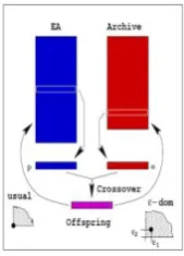
-MOEA algorithm

Here we use

𝜖

-dominated multi-objective evolutionary algorithm which was introduced by Deb (2001) [16]. The search space is divided into a number of grids (or hyper-boxes) and diversity is maintained by ensuring that a grid or hyper-box

can be occupied with only one solution. In this type of MOEA, there are two co-evolving populations: the EA population P(t) and the archive population E(t) (where 𝑡 is the iteration counter) as shown in Figure 4. MOEA starts with an initial population

P(0). The archive population E(0) stores the non-dominated solutions. Then, two solutions are selected from each population for mating. To select a solution from P(t), two members of the parent population are randomly selected and a domination check (in the usual sense) is made (As shown in the left side of Figure 3 for minimization of the objective function).

If one solution dominates the other, the former is selected. Otherwise, the two solutions are non-dominated to each other and we simply choose one of the solutions at random. We denote the chosen solution with 𝑝. To select the solution 𝑒 from E(t),

several strategies involving a certain relationship with 𝑝 can be made. However, here we randomly take a solution from E(t). After this selection phase,

solutions 𝑝 and 𝑒 are mated to create 𝜆 offspring solutions (𝑐𝑖. 𝑖 = 1.2. … . 𝜆). We displayed the

instance 𝜆 = 1 in the figure and used this value in all the simulations with 𝜖-MOEA in this article. Now,

each of these offspring solutions is compared with the archive and the EA population for their possible inclusion. For inclusion in the archive, the offspring

𝑐

_𝑖 is compared with each member in the archive for

𝜖

-dominance. Every solution in the archive is assigned an identification array (𝐵) as follows:

𝐵𝑗(f) = {

⌊𝑓𝑗− 𝑓𝑗

min

𝜖𝑗⌋

. for minimizing 𝑓𝑗.

⌈(𝑓𝑗− 𝑓𝑗min )/𝜖𝑗⌋. for minimizing 𝑓𝑗.

where 𝑓_𝑗min is the minimum possible value of the 𝑗

-th objective and 𝜖𝑗 is the allowable tolerance in the 𝑗-th objective beyond which two values are

significant to the user. This 𝜖_𝑗 value is similar to the

𝜖 used in the 𝜖-dominance definition. The

identification arrays make the whole search space into grids having

𝜖

𝑗 size in the

𝑗

-th objective.

Figure 3. 𝜖-MOEA procedure, the minimization of an

(4)

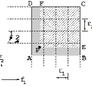
Figure 4 shows that the solution P𝜖-dominates the

entire region ABCDA (in the minimization sense), while the original dominance definition allows P to

dominate only the region PECFP.

Figure 4. The 𝜖-dominance concept (for minimizing 𝑓1

and 𝑓2).

For the sake of brevity, the rest of the discussion is only limited to minimization instances. However, a similar analysis can be done for maximization or mixed instances as well. The identification array of

P is the coordinate of point A in the search space. With the identification arrays calculated for offspring 𝑐_𝑖 and each archive member 𝑎, we use the following procedure. If the identification array B_𝑎 of any archive member 𝑎 dominates that of offspring 𝑐_𝑖, it means that the offspring is 𝜖-dominated by the archive member and the offspring is not accepted. However, if B_𝑐 of the offspring dominates B_𝑎 of any archive member 𝑎, those archive members are

deleted and the offspring is accepted. If neither of the above cases happens, it means that the offspring is 𝜖-non-dominated with the archive members. If

the offspring dominates the archive member or if the offspring is non-dominated to the archive member but is closer to the B vector than the

archive member (in terms of the Euclidean distance), the offspring is retained. In case an offspring does not share the same B vector with any archive member, the offspring is accepted. Interestingly, the former condition ensures that only one solution with a distinct B vector exists in each hyper-box, that is, each hyper-box on the Pareto-optimal front can be occupied by exactly one solution, thereby providing two properties: (1) well-distributed solutions are retained, and (2) the archive size will be bound. Therefore, no specific upper limit needs to be set on the archive size. The archive will be bounded according to the chosen 𝜖 -vector. The decision whether or not an offspring will replace any population member can be made using different strategies. Here, we compare each offspring with all population members. If the offspring dominates any population member, it replaces the member. However, if any population member dominates the offspring, it is not accepted. When both the above tests fail, the offspring replaces a randomly selected population member. This ensures that the EA population remains unchanged. This procedure is continued for a

specific number of iterations and the final members of the archive are reported as the obtained solutions. The proposed algorithm has the following properties:

1.It is a steady-state MOEA.

2.It emphasizes non-dominated solutions. 3.It maintains diversity in the archive by allowing

only one solution to be present in each pre-assigned hyper-box on the Pareto-optimal front. 4.It is an elitist approach.

4. Methodology

185 companies listed in Tehran Stock Exchange (TSE) were selected from a total population 452 companies. The financial data of these companies for a three-year period (2009-2011) comprised the input data. After initial processing in Excel Software, the data were imported into MATLAB for further analyses. First the shares of each of these companies were assigned a weight from 1 to 100. After determining the weights of companies, a 10-share optimal portfolio was generated from 185 companies. The constraints of the problem were:

1.The sum of ratios (weights) equals 1

2.Second constraint: There are exactly 10 assets in each portfolio (𝑘 = 10)

3.Third constraint: If an asset is placed in the portfolio then 𝛿_𝑖= 1 and its weight lies between

𝑙_𝑖 and 𝑢_𝑖; if the assets is not placed in the portfolio then 𝛿𝑖= 0 and its weight will be zero.

Satisfaction of constraints: 1.Beginning the algorithm

2.Problem parameters: At this stage the parameters and the main problem are examined.

• Reading the problem: 𝜎, 𝜇, sample size, K = 10, and 𝑙𝑖 and 𝑢𝑖 as the lower and upper bounds of

the portfolio that take a vale from 0.01 to 1.

• Calculating risk which obtained from the covariance of the expected returns of each company. Therefore, a 50 × 185 matrix is

created with entries that correspond to these expected returns.

• Determining the initial population with 50 random chromosomes.

• The iteration process must be five times the initial population.

• Two objective functions 𝑓₁ and 𝑓₂

min 𝑝(𝑥) = ∑ ∑ 𝑥𝑖𝑥𝑗𝛿𝑖𝑗 𝑛

𝑗=1 𝑛

𝑖=1

max 𝜇(𝑥) = ∑ 𝑥𝑖𝜇𝑖

𝑛

𝑖=1

• The genes in each chromosome is 185 (𝑁 = 185)

(5)

generated where 50 is the number of chromosomes and 185 is the number of companies. The entries in this matrix are random weights between 0.01 and 1 (lower and upper bounds of the problem).

𝑤₁= [

𝑥_1×1 𝑥_1×2 ⋯ 𝑥_1×185

⋮ ⋮ ⋯ ⋮

𝑥_50×1 𝑥_50×2 ⋯ 𝑥_50×185

]

50×18

Then, 10 more weights are selected in each row and the rest of the entries are zeroed. Therefore, the second constraint on the number of portfolio shares is satisfied (K = 10).

𝑤2= [

0.5 0 0.3 ⋯

⋮ ⋱ ⋮

]

50×18

Then the binary matrix (∆) is created where companies with weight take a value of 1 and companies without weight take a value of 0.

∆= [

1 0 0 1 1 0 1 ⋯

⋮ ⋮ ⋮

]

50×185

Now the initial population is evaluated. The evaluation rate is calculated as follows:

𝑋 = li. 𝛿 + 𝑤. 𝛿

∑𝑛𝑖=1𝑤. 𝛿

(1 − ∑ 𝑙. 𝛿)

𝑛

𝑖=1

. 𝑖 = 1. … . 𝑛

This rate calculates the real weights of the portfolio whose sum equals 1 (the first constraint).

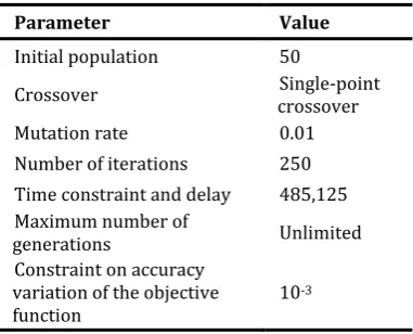
Table 1. The parameters of 𝜖-MOEA.

Parameter Value

Initial population 50

Crossover _crossoverSingle-point

Mutation rate 0.01

Number of iterations 250 Time constraint and delay 485,125 Maximum number of

generations Unlimited

Constraint on accuracy variation of the objective

function 10

-3

Considering the objective function and the defined constraints, a portfolio is generated from the superior shares which not only has the maximum expected return, but also minimizes risk.

Figure 5 displays the approximate shape of the efficient frontier obtained through the proposed procedure along with the cardinality constrained efficient frontier (TCCEF). TCCEF contains 185 efficient points that have been calculated using the model and algorithm explained earlier. It can be observed that

𝜖

-MOEA has calculated the efficient frontier in a way that approximates the efficient points obtained from the mathematical method (Figure 5).

Figure 5. The efficient frontier obtained from TCCEF and 𝜖-MOEA.

5. Conclusion

The present research is in the area of accounting and is carried out based on the stock market data and financial statements of companies. First, the data were collected from the software provided by Tehran Stock Exchange that contained the financial statements of the listed companies. Then, the data were analyzed in Excel and MATLAB applications. Finally, the optimal portfolio was generated suing

MVCCPO and the efficient frontier was obtained using the standard Markowitz procedure as well as

𝜖

-MOEA. As can be seen in Figure 5, these efficient frontiers coincide, suggesting that the proposed algorithm has been successful in solving the portfolio optimization problem.

References

1.Markowitz, H. 1952. Portfolio selection. The

(6)

2.Markowitz, H, 1959. Portfolio Selection: Efficient Diversification of Investments. New York: John Wiley & Sons.

3.Chang, T. J., N. Meade, J. E. Beasley, Y. M. Sharaiha. 2000. Heuristics for cardinality constrained portfolio optimisation. Computers & Operations

Research 27(13): 1271–1302.

4.Alexander, J. G., A. M. Baptista. 2001. Economic implications of using a mean-VaR model for portfolio selection: A comparison with mean-variance analysis. Journal of Economic Dynamics and Control 26(7-8): 1159-1193.

5.Hanne, T. 2007. A multiobjective evolutionary algorithm for approximating the efficient set. European Journal of Operational Research 176(3): 1723-1734.

6.Abdelaziz, F., B. Aouni, R. E. Fayedh. 2007. Multi-objective stochastic programming for portfolio selection. European Journal of Operational

Research 177(3): 1811–1823.

7.Ehrgott, M., K. Klamroth, C. Schwehm. 2004. An MCDM approach to portfolio optimization. European Journal of Operational Research 155(3): 752-770.

8.Best, M. J., J. Hlouskova. 2006. Quadratic programming with transaction costs. Computers &

Operations Research 35(1): 18–33.

9.Yu, L., X. Yao, S. Wang, K. K. Lai. 2011. Credit risk evaluation using a weighted least squares SVM classifier with design of experiment for parameter

selection. Expert Systems with Applications 38(12): 15392–15399.

10.Roy, A. D. 1952. Safety first and the holding of assets. Econometrics 20: 431-449.

11.Huang, X. 2008. Portfolio selection with a new definition of risk. European Journal of Operational Research 186(1): 351-357.

12.Lin, P. C., P. C. Ko. 2009. Portfolio value-at-risk forecasting with GA-based extreme value theory. Expert Systems with Applications 36(2): 2503-2512.

13.Anagnostopoulos, K. P., G. Mamanis. 2011. The mean–variance cardinality constrained portfolio optimization problem: An experimental evaluation of five multi objective evolutionary algorithms. Expert Systems with Applications 38 (11): 14208–14217.

14.Danayifar, H., S. M. Alvani. 2004. Quantitative Research Methodology in Management: A Comprehensive Approach, 2rd Edn. Saffar Publications, Tehran.

15.Deng, G. F., W. T. Lin, C. C. LO. 2012. Markowitz-based portfolio selection with cardinality constraints using improved particle swarm optimization. Expert Systems with Applications 39(4): 4558–4566.