Export Led Growth in Tunisia: A wavelet filtering based analysis

Munich Personal RePEc Archive

Export-Led Growth in Tunisia: A

wavelet filtering based analysis

Hamrita, Mohamed Essaied

Heigh Institute of Applied Mathematics and Informatics

5 January 2014

Online at

https://mpra.ub.uni-muenchen.de/52722/

Export-Led Growth in Tunisia: A wavelet filtering

based analysis

Mohamed Essaied Hamrita

High Institute of Applied Mathematics and Informatics,

Department of Mathematics, Street Ibn Fourat, 3100 Kairouan, Tunisia.

[email protected]

Abstract

In this paper, we use a wavelet filtering based approach to study the econo-metric relationship between exports, imports, and economic growth for Tunisia, using quarterly data for the period 1961:1-2007:4. GDP is used as a proxy for eco-nomic growth. We explore the interactions between these primary macroecoeco-nomic inputs in a co-integrating framework. We also study the direction of causality between the three variables, based on the more robust Toda-Yamamoto modified Wald (MWALD) test. The much-studied relationship between these three primary indicators of the economy is explored with the help of the wavelet multi-resolution filtering technique. Instead of an analysis at the original series level, as is usually done, we first decompose the variables using wavelet decomposition technique at various scales of resolution and obtain relationship among components of the de-composed series matched to its scale. The analysis reveals interesting aspects of the interrelationship among the three fundamental macroeconomic variables.

Keywords: Export, economic growth, cointegration, wavelet filtering, causality.

1

Introduction

to trade is also central in international negotiations about trade and tariff barriers where trade theory suggests that all parties on aggregate will enhance their welfare position in relation to their autarky situation. An export-led growth (ELG) hypothesis which states that exports are keys to promoting economic growth provides one of the answers to this fundamental question. There is a considerable literature that investigates the link and causation between exports and economic growth, but the conclusions still remain a subject of debate.

A number of empirical studies have documented a strong and positive relationship

be-tween export and economic growth including [Balassa(1978)], [Jung, W.S. and P.J. Marshall (1985)], [Chow(1987)], [Ahmad and Kwan(1991)], and [Moosa (1999)] among others. The results

reveal evidence in support of the export-led growth hypothesis for various countries. Sev-eral studies have also shown that it is possible to have growth-led exports (GLE) which has the reverse causal flow from economic growth to exports growth. In the GLE case, ex-port expansion could be stimulated by productivity gains caused by increases in domestic levels of skilled-labor and technology [Bhagwati (1988)], [Krugman (1984)]. The third alternative is that of import-led growth (ILG) which suggests that economic growth could be driven primarily by growth in imports. Endogenous growth models show that imports can be a channel for long-run economic growth because it provides domestic firms with access to needed intermediate factors and foreign technology [Coe and Helpman(1995)]. Growth in imports can serve as a medium for the transfer of growth-enhancing foreign R&D knowledge from developed to developing countries [Joy, M (2001)].

In this paper, we use a wavelet filtering based approach to study the econometric relationship between exports, imports and gross domestic product (GDP). We explore the interactions between these primary macroeconomic indicators in a co-integrating and vector auto-regression framework and their dynamic causality under the augmented level VAR setup. The much studied relationship between these three primary indicators of the economy is explored with the help of the wavelet multi-resolution filtering technique. Instead of an analysis at the original series level, as is usually done, we first decompose the variables using wavelet decomposition technique at various scales of resolution and obtain relationship among components of the decomposed series matched to its scale. The analysis reveals interesting aspects of the interrelationship among the three funda-mental macroeconomic variables.

This paper contributes to the literature on the export-out growth nexus in the follow-ing ways. First, previous studies on the dynamic linkages between exports and economic growth are extended through the application of wavelet transform and through the appli-cation of recent advance in time series statistical technique (augmented level VAR model-ing with integrated and co-integrated process of arbitrary orders [Toda and Yamamoto (1995)] and [Dolado and Lutkepohl(1996)]). In addition to employing recently developed time series modeling techniques, this study also expands on the three variables to include exports, imports and economic growth.

and section 4 summarizes the paper’s findings.

2

Analytical framework and methodological issues

2.1

Background on Wavelets

In this section we give a brief exposition of the relevant aspects of wavelet theory, with-out going into deeper detail abwith-out the mathematical involved. For precise mathematical statement we refer the reader to [Meyer (1990)], [Mallat (1989)], [Daubechies (1992)], [Chui(1992)], [Percival and Walden (2000)], [Genacy et al. (2002)] and [Nason (2000)].

Wavelets are building block functions and localized in time or space. They are ob-tained from a simple functionψ(t), called the mother wavelet, by translations and dila-tions. The wavelet ψ_j,k is obtained from the mother wavelet by shrinking by a factor of 2j _{and translating by 2}j_{k to obtain}

ψj,k(t) = 2j/2ψ(2jt−k) (1)

Except in some special cases, there is no analytic formula for computing wavelet func-tions. To evaluate a wavelet function, use the dilation equation

φ(t) = √2X

k

lkφ(2t−k) (2)

where φ(t) is the so called scaling function (or father wavelet), satisfying R_Rφ(t)dt = 1. We can obtain the mother wavelet ψ(t) from the father wavelet through

ψ(t) =√2X

k

hkφ(2t−k) (3)

with hk = (−1)kl1−k, called the quadrature mirror filter relation, where the coefficients lk and hk are the low-pass and high-pass filter coefficients defined as

lk =

√

2

Z

R

φ(t)φ(2t₋k)dt (4)

and

hk =

√

2

Z

R

ψ(t)φ(2t₋k)dt (5) For the wavelet series representation of a function, we expand the function in terms of some orthonormal base different from the trigonometric base. The standard wavelet series representation in terms of basis functions is given by:

f(t) = X

k

c_j0,kφj0,k(t) +

X

j≥j0

X

k

d_j,kψ_j,k(t) (6)

c_j0,k =

Z

R

f(t)φ_j0,k(t)dt and dj,k =

Z

R

f(t)ψ_j,k(t)dt

j0 is called thecoarest scaleof the wavelet representation,φj0,k(t) is an orthonormal basis

function given by

φj0,k(t) = 2

j0/2

φ(2j0t−k) (7)

Wavelet decomposition is usually obtained using an algorithm referred to as the Mallats Pyramid algorithm [Mallat (1989)]. This algorithm due to Mallat consists of a sequence of application of low-pass and high-pass filters.

The procedure starts with the datac0 = (c0,0, . . . , c0,T−1)′, wherec0,i=Xi, i= 0, . . . , T−

1. In theJ-th step, the algorithm computes c_j,k and d_j,k from the smooth coefficients of level j₋1,cj−1,k through

cj,k =

X

n

l2k−ncj−1,n (8)

d_j,k = X

n

h2k−ncj−1,n (9)

2.2

Unit root test

A unit root test tests whether a time series variable is non-stationary using an

autoregres-sive model. The most famous test is the Augmented Dickey-Fuller test [Dickey and Fuller(1979)]. Another test is the Phillips-Perron test [Philips and Perron (1988)]. The ADF and PP

unit root tests are for the null hypothesis that a time series y_t is I(1). Stationarity tests, on the other hand, are for the null that yt is I(0). The most commonly used

sta-tionarity test, the KPSS test, is due to Kwiatkowski, Phillips, Schmidt and Shin (1992) [Kwiatkowski et al. (1991)].

2.3

Cointegration analysis

The second stage involves testing for the existence of a long-run equilibrium relationship between real exports, real imports and GDP within a multivariate framework.

Further, we explore a co-integrating relationship among the variables. We first con-sider co-integration testing in a univariate time series setup. If a time seriesYt, with no

deterministic component, can be represented by a stationary and invertible ARMA pro-cess after differencingdtimes, the series is said to be integrated of orderd, i.e.,Yt∼I(d).

Furthermore, if all elements of a vector time seriesYt are I(d) and there exists a vector β ₆= 0 such that βT_Y

t ∼ I(d−b) for any b > 0, the vector process is said to be

The standard procedure for testing co-integration is through Engel-Granger test [Granger, C.W.J (1987)]. The test is a two-step procedure where ifX1, X2, . . . , Xk are k I(1) variables. Then first

we find the OLS regression of say, X1 on (X2, . . . , Xk), i.e., X1t =α+β1X2t+. . .+βk−1Xkt+εt

Next we apply stationarity test, like the ADF test on the estimated residuals and infer that (X1, X2, ..., Xk) is a set of co-integrated variables if and only if the estimated

residu-als are stationary. The co-integrating vector in such a situation is (1,₋β1,−β2, . . . ,−βk−1).

The long run equilibrium relationship between the variables beingX1 =α+β1X2+. . .+

βk−1Xk.

Existence of con-integration can also be tested under VAR setup. The VAR based con-integration testing is known as the Johansen’s tests. Under the VAR setup, we consider the vector autoregressive formulation with stationary errors

Y_t =µ+

p

X

i=1

φ_iY_i−1+εt (10)

The first difference formulation of the above model is

∆Yt=µ+ Γ1∆yt−1+ Γ2∆yt−2+. . .+ Γp−1∆yt−p+1+ ΠYt−p+εt

where

Γi = (φ1+φ2+. . .+φi)−Ik; for i= 1,2, . . . , p−1

and

Π = (φ1 +φ2+. . .+φi)−Ik

The matrix Π contains information on possible co-integrating relations between k ele-ments of Yt. Rank(Π) equals the number of independent co-integrating vectors of the

system. Number of distinct co-integrating vectors can thus be obtained by checking the significance of the characteristic roots of Π. [Johansen, S (1988)] uses maximum likeli-hood based approach for testing the number of characteristic roots that are significantly different from zero.

Johansen’s ”Trace Test” procedure sequentially tests the following hypotheses:

H00 : r= 0 vs H 0

A:r ≥0 H01 : r≤1 vs H

1

A:r ≥2

...

H0k−1 : r ≤k−1 vs H

k−1

A :r =k

wherer denotes the number of co-integrating vectors in the system. Johansen’s ”Trace Statistics”, for testing the rth hypothesis is given by

λ_trace(r0) =−T

k

X

i=r0+1

where T is the sample size and bλi are the estimated eigenvalues of the matrix Π. If

rank(Π) =r0 thenbλr0+1, . . . ,bλkshould all be close to zero andλ_trace(r0) should be small.

In contrast, if rank(Π)> r0 then some of bλr0+1, . . . ,bλk will be nonzero (but less than 1)

and λ_trace(r0)) should be large. The asymptotic null distribution of λtrace(r0) is not

chi-square but instead is a multivariate version of the Dickey-Fuller unit root distribution which depends on the dimensionn₋r0 and the specification of the deterministic terms.

Then the ”maximum eigenvalue” test statistic for testing therth hypothesis is given by

λmax(r0) = −Tlog(1−bλr0+1) (12)

As with the trace statistic, the asymptotic null distribution ofλmax(r0) is not chi-square

but instead is a complicated function of Brownian motion, which depends on the dimen-sion n₋r0 and the specification of the deterministic terms.

2.4

Causality relationships

Causality denotes a necessary relationship between one event (called cause) and another event (called effect) which is the direct consequence of the first. In others words, whether one variable can help forecast another variable or not.

One way to address this question was proposed by [Granger, C.W.J (1987)] and popular-ized by Sims [Sims, C.A (1972)]. Testing causality, in the Granger sense, involves using F-tests to test whether lagged information on a variable Y provides any statistically significant information about a variableX in the presence of lagged X. If not, then ”Y

does not Granger-causeX”. Here, assuming a particular autoregressive lag length p, we estimate the following unrestricted equation by ordinary least squares (OLS):

Xt =µ+ p

X

i=1

αiXt−i+ p

X

i=1

βiYt−i+ut (13)

The null hypothesis under this setup of causality testing is framed as

H0 : Y does not Granger-cause X.

In terms of model (Equation 13), we are interested in testing the following hypothesis

H′

0 : β1 =β2 =. . .=βp = 0.

This is the simultaneous testing of a subset of regression parameters and can be tested using usual F-statistic. It is worth noting that with lagged dependent variables, as in Granger-causality regressions, the test is valid only asymptotically. The test procedure can be extended to cover the causality situation involving groups of variables.

The [Toda and Yamamoto (1995)] procedure uses a modified Wald (MWALD) test to test restrictions on the parameters of the VAR(k) model. This test has an asymptotic chi-squared distribution withkdegrees of freedom in the limit when a VAR [k+d(max)] is estimated (whered(max) is the maximal order of integration for the series in the sys-tem). Two steps are involved with implementing the procedure. The first step includes determination of the lag length (k) and the maximum order of integration (d) of the variables in the system. Measures such as the Akaike Information Criterion (AIC) and Hannan-Quinn (HQ) Information Criterion can be used to determine the appropriate lag structure of the VAR. Given the VAR(k) selected, and that the order of integration

d(max) is determined, a level VAR can then be estimated with a total ofp= [k+d(max)] lags. The second step is to apply standard Wald tests to the firstkVAR coefficient matrix (but not all lagged coefficients) to conduct inference on Granger causality.

3

Empirical results

3.1

Data description and descriptive statistics

For the present study, we have considered Tunisian macroeconomic time series data on ex-ports, imports and GDP index. The data set,obtained from the National Statistics Insti-tute of Tunisia, is quarterly and covers the periods 1961:1-2007:4. All the variables are in natural logarithms. The definitions of variables are the following: X = ln Real Exports,

M = ln Real Imports and GDP = ln Gross Domestic Product.

The descriptive statistic is given in the (Table 1). From this table, the mean is not

signifi-mean std.dev skewness kurtosis JB p.value Y 3.1171 0.0512 -0.5492 -1.0741 18.2965 0.0001 X 3.0664 0.0688 -0.5950 -1.0281 19.2133 0.0001 M 3.0659 0.0773 -0.7715 -0.8498 24.3055 0.0000

Table 1: Summary statistics

cantly different from zero for either series. Normality is tested with the Jarque-Bera test, distributed asχ2

(2) under the null hypothesis, so is strongly rejected for all series. Since rejection could be due to either excess kurtosis, or skewness. We report these statistics, separately in the (Table 1).

Figure 1: GDP, Exports and Imports series

3.2

Wavelet decomposition

We first obtain a wavelet decomposition of the respective macroeconomic series. All the wavelet decompositions are done using a Daubechies extremal phase filters of length

re-lationships. We observe that the approximation series, corresponding to a level 3 de-composition of each of the macroeconomic indicators results in reasonable smoothing1

The application of the translation invariant wavelet transform with a number of scales

J = 3 produce three vectors of details coefficients, that isd1, d2 andd3,, and one vector of

wavelet smooth. The vectors of details coefficients corresponding to this decomposition represent the short-term fluctuations and are stationary and hence do not contain any deterministic information about the respective series. Econometric analysis, as discussed in the following section, is carried out on the level 3 approximation series, which repre-sent the smooth components of the respective macroeconomic indicators. In Figure 2,

Figure 3, and Figure 4 we report the wavelet decomposition of series.

Figure 2: Wavelet decomposition of Exports series

1_{In general, J is the highest resolution level such that 2}J

Figure 4: Wavelet decomposition of GDP series

3.3

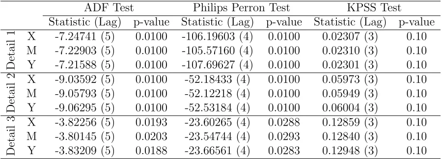
Test results for unit roots

ADF Test Philips Perron Test KPSS Test Statistic (Lag) p-value Statistic (Lag) p-value Statistic (Lag) p-value

X -2.08588 (5) 0.48641 -1.96583 (4) 0.95592 4.47958 (3) 0.01000

M -1.91339 (5) 0.56832 -1.50448 (4) 0.97650 4.31119 (3) 0.01000

Y -1.85945 (5) 0.59555 -1.43931 (4) 0.97571 4.53364 (3) 0.01000 ∆X -3.42928 (5) 0.05154 -28.65515 (4) 0.01000 0.37662 (3) 0.08723 ∆M -3.89190 (5) 0.01589 -31.51380 (4) 0.01000 0.56147 (3) 0.02782 ∆Y -3.20722 (5) 0.08855 -28.38377 (4) 0.01000 0.51762 (3) 0.03770 Table 2: Unit root test results of level 4 approximation series and their first difference series

Export, Import and GDP are all order one integrated, i.e. I(1) time series processes.

ADF Test Philips Perron Test KPSS Test

Statistic (Lag) p-value Statistic (Lag) p-value Statistic (Lag) p-value

D

et

ai

l

1 _{X -7.24741 (5) 0.0100 -106.19603 (4) 0.0100 0.02307 (3) 0.10}

M -7.22903 (5) 0.0100 -105.57160 (4) 0.0100 0.02310 (3) 0.10 Y -7.21588 (5) 0.0100 -107.69627 (4) 0.0100 0.02301 (3) 0.10

D

et

ai

l

2 _{X -9.03592 (5) 0.0100 -52.18433 (4) 0.0100 0.05973 (3) 0.10}

M -9.05793 (5) 0.0100 -52.12218 (4) 0.0100 0.05949 (3) 0.10 Y -9.06295 (5) 0.0100 -52.53184 (4) 0.0100 0.06004 (3) 0.10

D

et

ai

l

3 _{X -3.82256 (5) 0.0193 -23.60265 (4) 0.0288 0.12859 (3) 0.10}

M -3.80145 (5) 0.0203 -23.54744 (4) 0.0293 0.12840 (3) 0.10 Y -3.83209 (5) 0.0188 -23.66561 (4) 0.0283 0.12948 (3) 0.10

Table 3: Unit root test statistics of the details time series

3.4

Cointegration test results

The cointegration tests were performed utilizing the Johansen [Johansen, S (1991)] and [Johansen, S (1995)] methodology. The Johansen methodology is a generalization of the Dickey-Fuller test. Two likelihood ratio tests, λ_{max and} λ_{trace, were used to test the}

hypotheses regarding the number of cointegrating vectors.

Before implementing the Johansen procedure for co-integration analysis, the auto-regression order of the VAR in Equation 10 has to be correctly specified. Therefore, to select the correct specification, we based our decision on the Schwarz Bayesian information crite-rion (BIC) and selectedp= 3.

the corresponding λ values. The maximum eigenvalue tests for at most r co-integrating vectors against the alternative of exactly r + 1, and the trace tests for at most r co-integrating vectors against an alternative of at least r+ 1 vectors.

[Johansen, S (1991)] discussed the likelihood based co-integration theory for such a

Trace test Max test

H0 λ Statistic p-value Statistic p-value

r = 0 0,12389 34,855 0,0112 24,469 0,0142

r _≤1 0,038899 10,387 0,2566 7,3401 0,4585

r _≤2 0,016333 3,0466 0,0809 3,0466 0,0809

Table 4: Johansen’s test for multiple cointegration vectors. Note that the p-values are computed via the approximations by[Doornik(1998)].

model without constant terms. It turns out, however, that the presence of a constant in the non-stationary part of the data generating process plays a crucial role in the statisti-cal analysis and for the interpretation of the model. In particular, [Johansen, S (1991)] proved that the asymptotic distribution of the test statistics and estimators in an error-correction model is not invariant to the assumption made about the constant term. [Osterwald (1992)] also proved that the distribution of the trace statistic could be af-fected by the presence of a constant term. Thus, we used the [Johansen, S (1995)] like-lihood ratio test to test whether the model should contain a constant term. The results of this test indicate that a model with an unrestricted constant should be adopted for the analysis. Both the maximum eigenvalue and trace statistics indicate the existence of a unique long-run relationship among the three endogenous variables included in the analysis.

3.5

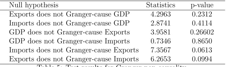
Test results for Granger Non-causality

Results from a VAR estimated using the procedure developed by [Toda and Yamamoto (1995)] are presented in Table 5.

For the purposes of this paper, the procedure is applied as follows:

1. Since the VAR model contains three lags and since the highest order of integration in the data is one, we first estimate a VAR in levels with four lags, then

2. We test jointly that the first three lags of the relevant variable are zero using a Wald test, which has a χ2

distribution.

between economic growth and export growth. This simultaneity arises from the fact that, at the initial stages of development, economic growth promotes exports, but along the way exports start generating the capital needed for further economic growth.

Null hypothesis Statistics p-value Exports does not Granger-cause GDP 4.2963 0.2312 Imports does not Granger-cause GDP 2.8741 0.4114 GDP does not Granger-cause Exports 3.9581 0.26602 GDP does not Granger-cause Imports 0.7346 0.8650 Imports does not Granger-cause Exports 7.3567 0.0613 Exports does not Granger-cause Imports 6.2653 0.0994

Table 5: Test results for Granger non-causality

4

Conclusion

In this chapter, we use the wavelet based filtering technique for establishing relationships among macroeconomic indicators of exports, imports and economic growth. An accu-rate analysis of co-integaccu-rated long-run equilibrium or causal relationships among these macroeconomic indicators is important. We consider the case of the Tunisian economy and explore and extract interesting relationships using wavelet technique. Using quar-terly data over the time period 1961:1-2007:4, after filtering the series using wavelet technique, we have analyzed the time series properties of the exports, imports and eco-nomic growth variables in order to determine the appropriate functional form for testing the ELG hypothesis.

The study find that, the exports, imports and GDP are co-integrated. From the causal-ity tests we have seen that there exist a bi-directional relationship between the Exports and GDP, no relevant causality between import and export growths at 10% level of significance and a bi-directional relationship between import and economic growths.

References

[Ahmad and Kwan(1991)] Ahmad, J and A.C.C. Kwan, Causality Between Exports and Economic Growth, Economics Letters, 37, 243-248,(1991).

[Balassa(1978)] Balassa, B, Exports and economic growth: further evidence, Journal of Development Economics, 5, 181 -189,(1978).

[Chow(1987)] Chow, P.C.Y, - Causality Between Export Growth and Industrial Perfor-mance: Evidence from the NIC’s, Journal of Development Economics, 26, 55-63, (1987).

[Chui(1992)] Chui, C.K, An Introduction to Wavelets, Academic Press, New York, (1992).

[Coe and Helpman(1995)] Coe, T.D and Helpman, E, International R&D spillovers, Eu-ropean Economic Review, 39, 859-887, (1995).

[Daubechies (1992)] Daubechies, I, Ten Lectures on Wavelets, Society for Industrial and Applied Mathematics, (1992).

[Dickey and Fuller(1979)] Dickey, D.A. and W.A. Fuller, Distribution of the Estimators for Autoregressive Time Series with a Unit Root, Journal of the American Statistical Association, 74, 427-431, (1979).

[Dolado and Lutkepohl(1996)] Dolado, J, J, and Lutkepohl, H, Making Wald test work for cointegrated VAR systems, Econometric Reviews, 15, 369-386, (1996).

[Doornik(1998)] Doornik, J, A - Approximations to the Asymptotic Distribution of Coin-tegration Tests, Journal of Economic Surveys, 12, 573-93, (1998).

[Genacy et al. (2002)] Genacy, R, Selcuk, F & Whitcher, B, An Introduction to Wavelets and Other Filtering Methods in Finance and Economics, Academic Press, New York, (2002).

[Granger, C.W.J (1987)] Granger, C.W.J, Coi-integration and error correction: repre-sentation, estimation and testing, Econometrica, 55, 251-276, (1987).

[Johansen, S (1988)] Johansen, S, Statistical Analysis of Cointegrating Vectors, Journal of Economic Dynamic and Control, 12, 231-254, (1988).

[Johansen, S (1991)] Johansen, S, Estimation and hypothesis testing of cointegration vectors in Gaussian vector autoregressive models, Econometrica, 59, 1551-80, (1991). [Johansen, S (1995)] Johansen, S, Likelihood Based Inferences in Cointegrated Vector

Autoregressive Models, Oxford: Oxford University Press, (1995).

[Joy, M (2001)] Joy, M, - Imported machinery and growth in LDCs, Journal of Develop-ment Economics, 65, 209-224, (2001).

[Krugman (1984)] Krugman, P.R, Import protection as export promotion, In: Kierzkowski, H. (Ed.), Monopolistic Competition in International Trade. Oxford University Press, Oxford, (1984).

[Kwiatkowski et al. (1991)] Kwiatkowski, D., P.C.B. Phillips, P. Schmidt and Y. Shin, Testing the Null Hypothesis of Stationarity Against the Alternative of a Unit Root, Journal of Econometrics, 54, 159-178, (1991).

[Mallat (1989)] Mallat, S, - A Theory for Multiresolution Signal Decomposition: The Wavelet Representation, IEEE Transactions on Pattern Analysis and Machine In-telligence, 11, 674-693, (1989).

[Meyer (1990)] Meyer. Y, Ondelettes et oprateurs I - Ondelettes, Hermann, (1990). [Moosa (1999)] Moosa, I, - Is the Export Led Growth Hypothesis Valid for Australia,

Applied Economics, 31, 903-906, (1999).

[Nason (2000)] Nason,G, Wavelet Methods in Statistics with R, Springer, (2000). [Osterwald (1992)] Osterwald-Lenum, M, A note with quantiles of the asymptotic

dis-tribution of the maximum likelihood cointegration rank test statistics: four cases, Oxford Bulletin of Economics and Statisitics, 54, 461-72, (1992).

[Percival and Walden (2000)] Percival, D. B and Walden, A. T, Wavelet Methods for Time Series Analysis, Cambridge University Press, (2000).

[Philips and Perron (1988)] Phillips, P, C, B and Perron, P, Testing for a unit root in time series regression, Biometrika, 75, 335-46, (1988).

[Sims, C.A (1972)] Sims, C.A, Money, income and causality, American Economic Re-view, 62, 540-552, (1972).

[Toda and Yamamoto (1995)] Toda, H,Y and Yamamoto, T, - Statistical inference in vector autoregressions with possibly integrated processes, Journal of Econometrics, 66, 225-250, (1995).