Coupled Kernel Ensemble Regression
Dickson Keddy Wornyo
Sch. Of Comp. Sci. and Telcomm. Eng.JiangSu University, Xuefu Road 301 Zhenjiang, Jiangsu, 212013, China
Elias Nii Noi Ocquaye
Sch. Of Comp. Sci. and Telcomm. Eng.JiangSu University, Xuefu Road 301 Zhenjiang, Jiangsu, 212013, China
Bright Bediako-Kyeremeh
Department Of Comp. Sci. Sunyani Technical University P. O. Box 206, Sunyani-BA, GhanaABSTRACT
In this paper, the concept of kernel ensemble regression scheme is enhanced considering the absorption of multiple kernel regrssors into a unified ensemble regression framework simultaneously and coupled by minimizing total loss of ensembles in Reproducing ker-nel Hilbert Space. By this, one kerker-nel regressor with more accurate fitting precession on data can automatically obtain bigger weight, which leads to a better overall ensemble performance. Comparing several single and ensemble regression methods such as Gradient Boosting, Support Vector Regression, Ridge Regression, Tree Re-gression and Random Forest with our proposed method, the ex-perimental results of the proposed model indicates the highest per-formances in terms with regression and classification tasks using several UCI dataset.
Keywords
Ensemble regression, Multi-kernel learning, Kernel regression
1. INTRODUCTION
Regression is a technique from fundamental statistic useful for pre-dicting outputs that are continuous. Regression techniques used for predicting data assimilation models have received a lot of active research hot spot in recent times, particularly in real-world applica-tions [6]. Presently, regression is portrayed as one of the most fun-damental big data statistical techniques utilized in solving issues of big data [5]. This help in predictions, in which both the sample size and the number of predictors are large for high-dimensional regressions. Additionally, it plays an important role in optimizing operations of complex systems due to its ability to forecast sys-tems behaviors [14]. As a result, regression techniques have been adopted in wide application areas, including but not limited to data mining, computer vision and medical image analysis [18]. Furthermore, a lot of strategies have been adopted in the execution of regression processes with diverse schemes. These schemes are mainly divided into two categories: single regression models and ensemble regression models [11]. The single regression model can also be sub grouped into non-linear and linear methods, whilst lin-ear regression, ridge regression and lasso regression among others are the representative examples of the non-linear method. For ex-ample, Santiago et al. [21] demonstrated the effectiveness of multi-variate linear regression models towards their application in vir-tual screening and mechanistic interrogation. Hellton et al. [12] also proposed the use of ridge regression with cross-validation as a plug-in estimate. Mangalathu et al. [19] proposed a
methodol-ogy to identify the relative impact of input variables and level of treatments needed in the estimation of seismic demand models and fragility curves using lasso regression.
On the other hand, linear methods, such as, kernel ridge regression and support vector regression (SVR) are widely known for their theoretical or experimental results. For example, Li et al. [17] pro-posed a kernel ridge regression with truncated Gaussian radial basis function kernel (KRR-TRBF) to train classifiers and further authen-ticates a current user as a legitimate user or an imposter. Cheng et al. [4] developed a full polynomial chaos expansion (PCE) meta-model based on an SVR technique using an orthogonal polynomi-als kernel function.
Besides, in the second broad category, ensemble regression model combines several decision trees to produce better predictive per-formance than utilizing a single decision tree. The main principle behind the ensemble model is that a group of weak learners come together to form a strong learner. This has yielded success in many real-world applications, such as decision tree regression, random forest regression and gradient boosting regression. For example, Hariharan et al. [9] explained how a random forest based model was used to estimate model parameters for modeling of a green-field terrain by non-deposit samples.
The Introduction of the Reproducing Kernel Hilbert Space (RKHS)[22] into the structure of the linear regression methods, sig-nificantly contributes to a higher performance result as compared with the non-linear regression methods. Thus the discrete relation-ship among data samples are characterized better. However, the se-lection of parameters has great influence on the performance of a single kernel regression method. The selection of a suitable kernel with their parameters is therefore a key problem for kernel regres-sion methods that must be greatly considered.
opti-mizes each base kernel regressor in separate RKHS and then cou-ples them into one regression model in multiple RKHSs whiles the existing coupling methods try to combine multiple RKHSs into one unified space.
The main contributions of this paper are as follows:
1. In the proposed method, base kernel regressors are coupled and co-optimized in a coupled ensemble framework by minimizing loss in multiple RKHSs. This is done without multiple RKHSs being combined into one unified space.
2. The coupled ensemble idea can find appropriate kernel types and their parameters in a base kernel regressor through a pool of ensemble regression framework, which is different from the state-art-of-work.
3. Additional experiments on artificial data sets, UCI regression and classification data sets indicate that compared to other re-gression methods, for example, random forest and SVR, the pro-posed method has the advantages of effective performances in keeping lowest regression loss and highest classification accu-racy
The rest of the paper is organized as follows: Section 2 introduces some related works with respect to the topic under discussion. Sec-tion 3 presents the proposed method. Experimental results are pre-sented in section 4. Finally, section 5 concludes the paper.
2. RELATED WORK
Regression learning has been addressed in a lot of prior studies. In this section, two main categories of regression have been in-troduced. Thus, single regression model and ensemble regression model. The single regression model is also classified into two sub categories: linear and non-linear methods
2.1 Non-linear methods
Lasso is a non-linear regression method that involves correcting the total size of the regression coefficients. Lasso regression is a regu-larization technique that’s useful for feature selection and to prevent over-fitting training data. It works by penalizing the sum of abso-lute value (L1 norm) of weights found by the regression. Wang et al. [24] proposed a lasso regression algorithm that employs variable selection for feature variables and further guide the trained predic-tor towards a generalization solution, thereby improving the accu-racy and interpretability of the model. Experimental results showed superiority prediction of fuel consumption compared to existing methods. Zhang et al. [27] recently proposed a locally weighted ridge regression method to overcome the problem of online sen-sitivity identification using ordinary regression methods that are prone to large errors.
Linear regression which is also an example of the non-linear meth-ods, attempts to model the relationship between two variables by fitting a linear equation to observed data. One variable is consid-ered to be an explanatory variable, and the other is considconsid-ered to be a dependent variable. Hirukawa et al.[13] demonstrated how the ordinary least square estimator of the linear regression model used matched samples of inconsistent and non-standard conver-gence rate to deal with earning data of missing observations to be imputed. Experimental results showed that the estimators had an indirect-inference interpretation and attained a parametric conver-gence rate when the number of matching variables is no greater than four.
2.2 Linear methods
The Introduction of the Reproducing Kernel Hilbert Space (RKHS) into the structure of the linear regression methods, significantly contributes to a higher performance result as compared with the non-linear regression methods. Thus the discrete relationship among data samples are characterized better. The nonlinear prob-lem is transformed into a linear probprob-lem through the application of different mathematical kernel functions. Representative kernel methods are kernel ridge regression and SVR methods.
Kernel ridge regression (KRR) is an instance of a natural exten-sion of ridge regresexten-sion and combines ridge regresexten-sion with ker-nel tricks. It thus learns a linear function in the space induced by the respective kernel and the data. For non-linear kernels, this cor-responds to a non-linear function in the original space. Chang et al. [2] proposed a kernel ridge regression (DSKRR) method based on divide-and-conquer strategy that provides error analysis for dis-tributed semi-supervised learning. Their results showed that the un-labeled data played an important role in reducing the distributed error and enlarging the number of data subsets in DSKRR. Support Vector Regression methods are the natural extension of SVM, proposed by Drucker [7]. SVR method is identical to ker-nel ridge regression base on their model forms. Chen et al. [3] pro-posed a three-layer weighted fuzzy support vector regression (TL-WFSVR) model for understanding human intention, and it is based on the emotion-identification information in human-robot interac-tion. Experimental results showed that the proposed TLWFSVR model obtained higher intention understanding accuracy and less computational time than that of the comparative methods. 2.3 Ensemble regression model
Ensemble regression (ER) can combine individual regressors to-gether and keep their performance better as compared to the sin-gle regression model. Tree regression method is used to predict the numerical outcomes of the dependent variables. Rathore et al. [20] presented a decision tree regression-based approach for the number of faults prediction in a given software module.
Furthermore, Gradient Boosting Decision Trees (GBDT) is an ad-dictive ensemble regression model in decision trees. Wang et al. [25] proposed a new fusion method based on the LR algorithm and GBDT algorithm for mobile recommendation system. Their method is observed to achieve a good F1 score in a mobile recom-mendation scenario.
Among ensemble regression methods, random forest (RF) method is a useful machine learning technique which can be applied in both regression and classification problems. Hasan et al. [10] applied random forest for intrusion detection problems. The research indi-cated that random forest takes less time to train its classifier than SVM and also achieves more accurate results than SVM classifier. Wu et al. [26] used random forest regression approach to analyze the weekly analysis of influenza-like illness rate using one year pe-riod of factors. Experimental results showed that regression errors decreased from 5.04% to 4.35% in mean absolute percentage error (MAPE) and 2.85E-04 to 1.97E-04 in mean square error (MSE) for prediction of weekly ILI rate.
3. THE PROPOSED METHOD
Kernel Hilbert Space (RKHS) and then the proposed coupled ker-nel ensemble regression method is proposed in the next subsection.
3.1 Reproducing Kernel Hilbert Space
Reproducing Kernel Hilbert Space is a special Hilbert space asso-ciated with a kernel such that it reproduces (via an inner product) each function in the space. It has a wide range of applications in machine learning, such as SVR and Radial Basis Functions [23]. Given data {{(xi, yi)}ni=1 ∈ Rp × Rp}, where Rp is a p -dimensional real space. A kernelkprovides a similarity measure between pairs of datapoints
k:Rp×Rp→R: (xi, yi)↔k(xi, yi) (1)
The set of these mappings can be extended by including all possible finite combinations, adjoining the limits and constructing an inner product base on the chosen kernel
ϕ(x)(x0) =hk(x,•), k(x0,•)i=k(x, x0) (2)
wherekhas a symmetric property that meansk(xi, x) =k(x, xi).
Some suitable functions can be regarded as kernels: -The Polynomial kernel
k(xi, xj) = (axTixj+b)c (3)
- The RBF kernel(Radial Basis Function)
k(xi, xj) =exp(−
kxi−xjk
µ ) (4)
- The Gaussian kernel
k(xi, xj) =exp(−
kxi−xjk2
2σ2 ) (5)
wherea, b, c, µ, σ ∈ R. Meanwhile,K denotes a Gram matrix which is obtained according to samples. It is a symmetric and semi-positive definite matrix, which can be shown as follows:
K=
k(x1, x1) k(x1, x2) · · · k(x1, xN)
k(x2, x1) k(x2, x2) · · · k(x2, xN)
..
. ... . .. ... k(xN, x1) k(xN, x2) · · · k(xN, xN)
(6)
The resulting RKHS has then the property that every evaluation operator and norm of any element inHkis bounded. For a Mercer
KernelK:χ×χ−→R, there is an associated RKHSHkof the
functionχ−→Rwith the corresponding normk kk.The standard
framework estimates an unknown function by minimizing
f∗=argmin
N X
i=1
ν(xi, yi, f) +ιkfk2k (7)
Whereν is a kind of loss function, such as squared loss(yi −
f(xi))2 for RLS or hinge loss function max[0,1−yif(xi]for
SVM.ιkfk2
k is regarded as a smoothness conditions on possible
solutions in the RKHS. In this case,it is proven that the optimal representer offin Eq.7 can be defined as a finite sum around the observations:
f=
N X
i=1
αik(xi, x) (8)
Therefore, the problem is reduced to optimizing over the finite di-mensional space or coefficientsαi, which is the algorithmic basis
for SVM and other kernel methods.
3.2 Coupled kernel ensemble regression
The proposed method can combine multiple kernel regressors into a unified ensemble regression framework and the weight of each kernel regressor in this ensemble method is coupled by minimizing total loss of ensembles in Reproducing Kernel Hilbert Spaces. This gives an advantage of one kernel regressor having more accurate fitting precession on data and can, therefore, obtain bigger weight which leads to a better overall ensemble performance
Firstly, different kernels are obtained according to samples. Sup-pose a regression problem has a training setXwith regression re-sult(X={(x1, y1), ...,
(xN, yN)}) and a testing set Xt without regression result
(Xt={(x1, ..., xNt)})where xn(xn ∈ R
d, n = 1, ..., N)
ex-presses a training sample,yn is the true regression result ofxn,
andxm(xm∈Rd, m= 1, ..., Nt)expresses a testing sample.N
is the number of training samples andNtis the number of testing
samples. The base kernel regression model is
kKα+b−yk2+λαTKα (9)
whereKdenotes a kernel matrix which can be obtained according to samples,αis a column vector related to the weight of every sam-ple,bexpresses bias term for the specificK.The proposed method aims to obtain the optimal co-regularized weight vector of base re-gressors. The termkKα+b−yk2is the square loss for determin-ing the performance of the base kernel regression model.
Unfortunately, since regression performance varies dramatically with the selection of both kernel functions and their parameters, it is also hard to obtain suitable Kernel functions and parameters which are commonly selected manually in practice. To overcome this problem, the proposed method can combine multiple kernel regressors into a unified ensemble regression framework without considering the selection of both kernel functions and their param-eters in individual kernel regressors. L different kernels are used in the proposed framework and a new coupled kernel ensemble re-gression model is proposed:
arg min
w,αi 1 2
L X
i=1
Wi(kKiαi+bi−yk
2
+λαiTKiαi)
s.t. 1TW = 1
(10)
WhereLis the number of kernels. Assuming that the number of training samples is N, and the number of testing samples is Nt
andW = [W1, ..., WL]Tdenotes a weight vector of individual
ker-nel regression model.Kirepresents the different kernel matrix.Ki
is the i-th base Gram matrix and the dimension ofKi isN×N
for training dataset,Nt×N for testing dataset.αidenotes a
col-umn vector related to the weight of every sample for eachKi. The
dimension ofαiisN×1for training dataset,Nt×1for testing
dataset.bi is the bias item for a specificKi.bi is a column
vec-tor that has the same dimension as samples, and each value in the vector is equal to a specificKi.ydenotes the true output and its
dimension is the same as samples.λis the constriction parameter that smoothens the model.
We take the derivative of formula 9 with respect toαiand obtain
the following formula.
αi= (Ki+λI)−1y (11)
According to Formula 11, we can get
bi=
1 N(
N X
t=1 yt−
N X
j=1
Ki(xj, xt)αi,j) (12)
We consideredWito beWir (rrepresents the control parameter
for the weights of multiple features) because linear programming attains its optimum solution at the extreme ends, i.e eitherWi= 0
orWi= 1. That means there will only be one kernel selected
con-trary to the proposed objective of exploring the rich complementa-tion of multiple kernels. Whenr= 1, it is only one kernel that will be selected in the optimal result, which is undesirable, but ifr >1 the outcome is based on multi-kernel balancing.ris a man-made value to obtain appropriatew. It can further be deduced as:
Wi=
(1
ζi)
r−1
L P
i=1 (1
ζi)
r−1 (13)
Whereζi=kKiαi+bi−yk
2
+λαiTKiαi denotes the loss of
each kernel. According to Eq, the optimal weight of the ensemble method can be obtained, where r is a parameter to obtain appro-priate w. An ensemble regresion model is obtain by combining the various base kernel models linearly. The proposed kernel ensemble regressor is built using the following formula 14
f(xt) = L X
i=1 Wi(
N X
j=1
Ki(xj, xt)αi,j+bi) (14)
4. EXPERIMENTAL RESULTS
In this section, all the experimental results under different settings are presented. For a fair comparison, each dataset is randomly split into 2/3 (training data) and 1/3 (testing data) and the regularization parameter is obtained by cross-validation method. In our experi-ments, five comparative methods (Gradient boosting, Tree Regres-sion, Support Vector RegresRegres-sion, Ridge Regression and Random Forest) are selected as base models. Mean Square Error (MSE) and Mean Absolute Error (MAE) are selected as the criteria [1].
M AE= 1 Nt
Nt
X
i=1
|f(xi)−yi| (15)
M SE= 1 Nt
Nt
X
i=1
(f(xi)−yi)
2
(16)
In the proposed method, a demonstration of how to combine the base kernel model of the ensemble is shown. A single polynomial kernel model in Eq.3 is applied as the basic model of the ensemble for different datasets.
[image:4.595.370.503.87.158.2]There are three parameters (a, bandc) in this type of model and the different values of the parameters show different effects on the experimental results. Generally, we seta ∈ {1∗1e−6,1∗ 1e−5,· · ·,1000},b∈ {1∗1e−6,1∗1e−5,· · ·,1000}and c∈ {1,2,3,4,5}. For each dataset, we select the optimal parame-ters (a, bandc) and base kernels are obtained by 10-fold cross vali-dation in experiments. The parameterLin Eq.10 denotes the num-ber of base polynomial kernel models. The generalization ability of an ensemble regressor will be good if there are enough base mod-els. However, excessive base models may consist of many worse base models and result in low classification accuracy. Therefore,
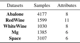
Table 1. : Descriptions of UCI dataset Datasets Samples Attributes
Abalone 4177 8
RedWine 1599 11
WhiteWine 1030 8
Mg 1385 6
Space 3107 6
we takeL∈ {10,20,50,100,150}. In our experiments, we select 20 combinations among three parameters (a, bandc).
And the parameter in Eq.10 is the parameter that smoothens the base regressor. The parameterrin Eq.13 is the control parameter for the weights of multiple base models. In our experiments, we select values forλandras 0.1 and 2, respectively.
4.1 Dataset description
The selection of nine benchmark publicly available datasets for the evaluation of the performance of the proposed model is made.These datasets are from the UCI database repository, a detailed summary is presented in Table 1.
4.2 Experimental settings
We compared the effectiveness and robustness of the proposed novel Kernel Ensemble Regression with the conventional multi-kernel features. The performances of some single and ensemble regression preserving methods such as Ridge Regression, Random Forest and Support Vector Regression among others are conducted but with careful tuning of the parameters. All the datasets selected are applied to these methods.
4.3 Performance Evaluations and comparisons
[image:4.595.114.283.468.540.2]This section discusses the general performance of the proposed co-regularized kernel ensemble regression algorithm and all the com-parative methods.
Table 2 shows the comparisons of the MSE mean of the CoKer, linear models and ensemble models. As shown in Table 2, the re-sult of CoKER on Abalone dataset is very small as compared to the other comparative methods. This indicates that, CoKER produces a smaller Mean Square Error (MSE) of 3.599 with respect to the abalone datasets. The tree regression model performs poorly with the highest MSE of 4.491. Considering the Red Wine dataset, all the comparative methods and CoKER yielded a positive result with respect to MSE. Nevertheless, CoKER performs best with an MSE of about 0.15% compared to the comparative methods. CoKER leads with a value of 56.0335 which is 3.42% better. It is then fol-lowed by ridge regression, while tree regression comes in with the least performance. Tree regression method has the worst perfor-mance of 6.4709 for this dataset.CoKER yields better results than the other methods in all the datasets except the Bodyfat dataset. Fi-nally, with a value of 0.022,CoKER leads the others on the Space dataset. From the MSE values presented in table 2, it demonstrates that for MSE values, CoKER proves beyond doubt to be the best method considering the comparative methods
Table 2. : The average of MSE comparison of CoKER, single models and ensemble models
Datasets CoKER GB TR SVR RR RF
Abalone 3.59 3.91 4.49 4.31 4.18 4.00
RedWine 0.41 0.42 0.50 0.61 0.44 0.43
WhiteWine 0.49 0.51 0.53 0.68 0.51 0.49
[image:5.595.56.300.98.168.2]Mg 0.013 0.016 0.022 0.0175 0.020 0.014 Space 0.022 0.024 0.032 0.039 0.024 0.023
Table 3. : The average of The MAE comparison of CoKER, single model and ensemble models
Datasets CoKER GB TR SVR RR RF
Abalone 0.124 0.134 1.026 1.170 0.174 4.002
[image:5.595.54.298.212.281.2]RedWine 0.051 0.061 0.397 0.517 0.100 0.070 WhiteWine 0.101 0.104 0.108 0.121 0.152 0.107 Mg 0.0007 0.001 0.011 0.035 0.002 0.001 Space 0.021 0.028 0.038 0.054 0.035 0.046
Table 4. : Descriptions of UCI classification dataset
Dataset Samples Attribute
Diabetes 768 8
German 1000 20
LD 345 7
Abalone 4177 8
Dexter 2600 20000
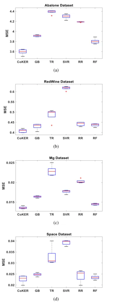
dataset, CoKER again performs better than the other methods with a value of 0.410. Gradient boosting is the second best performer while SVR has the worst lower bound performance. Fig 1(a) and 1(c) shows a lot of flat shaped plot. This implies that, when the re-gression variance becomes smaller, the more stable the method, and the lower the median, the better the regression result of the method. This because most of the variance is very small,i.e.,10−4and could not be shown in the tables.. Here, CoKER again performed better than the rest of the methods.
From the above discussion, it can conclude that the propose CoKER outperforms the comparative methods.
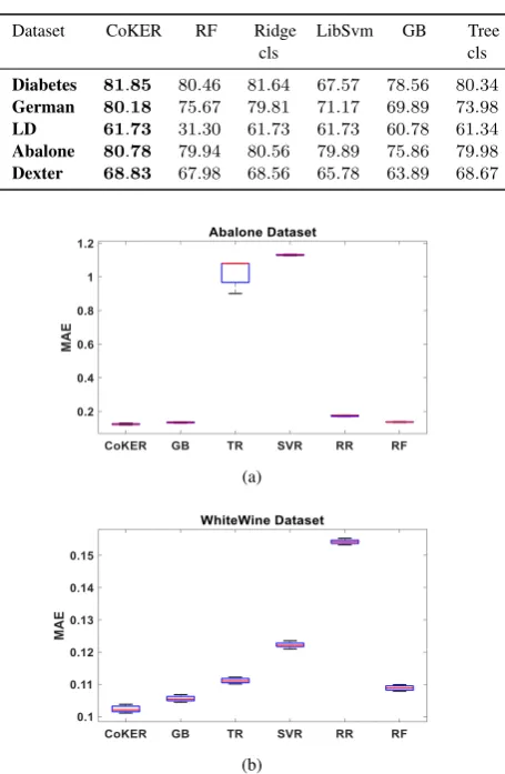
Table 3 presents the mean MAE comparisons among the propose CoKER, linear models and ensemble models. From the results, it can be seen that, when applied to the Abalone dataset, the CoKER attains the optimal result of 0.1245. Gradient boosting lags slightly behind by 0.01% with a value of 0.134. Random forest yields the worst result with a value of 4.002. When applied to WhiteWine, CoKER performs better than other methods by 1.17%. CoKER pro-vides the best result with a value of 0.134 which is 35% better than the others. CoKER, when applied to Mg turns out to be the best performer with a value of 7.0000e-04 and gradient boosting being the worst performer with a value of 0.001. The Space dataset had the proposed method performing better than the others by 1.3%. It could be seen from the results in table 3 that the propose CoKER has better MAE values compared with the prior studies on the var-ious datasets. From the experimental results, it could be realized that, the propose CoKER outperforms the prior approaches in all experiments.
Figure 2 also gives a different view of MAE comparisons among the propose CoKER, single models and ensemble methods. From
(a)
(b)
(c)
(d)
Fig. 1: Box Plot of the respective datasets for MSE: (a) Abalone (b) Red-wine (c) Mg (d) space
[image:5.595.113.235.313.384.2]Table 5. : The comparison of classification mean accuracies of CoKer com-parative methods, (cls = classification)
Dataset CoKER RF Ridge LibSvm GB Tree cls cls
Diabetes 81.85 80.46 81.64 67.57 78.56 80.34 German 80.18 75.67 79.81 71.17 69.89 73.98 LD 61.73 31.30 61.73 61.73 60.78 61.34 Abalone 80.78 79.94 80.56 79.89 75.86 79.98 Dexter 68.83 67.98 68.56 65.78 63.89 68.67
(a)
[image:6.595.58.286.92.441.2](b)
Fig. 2: Box Plot of the respective datasets for MAE: (a) Abalone (b) WhiteWine
median of the method in the figure, the better the regression result of the method. This because most of the variance is very small,i.e., 10−4and did not show them in the tables.
From the above discussion, it can conclude that, the proposed CoKER demonstrates more effectiveness and superiority than the prior studies in regression accuracy.
4.4 Classification
Although all the models discussed in the previous section are in-tended for regression tasks, classification task is also experimented to further verify the stability of the proposed model.
4.5 Data description
The selection of nine benchmark publicly available datasets for the evaluation of the performance of the proposed model is made, which are Diabetes, German, Liver-disorders (LD), Abalone, and Dexter. A summary is presented in Table 4.
Table 5 did not present the variance of the experiment because they were very small, of about10−4. which means the smaller the
vari-Fig. 3: Comparison of the mean classification accuracies of the various datasets across the five comparative methods
ance, the more stable the method and the lower the median of the method in the table, the better the classification result of the method Fig. 3 presents a comparison of the mean classification accuracies of all the methods across the five datasets. From the figure it can see that, the propose CoKER obtains the highest accuracy of 81.86% on the diabetes dataset, followed closely by Ridge Classification method with an accuracy of 81.66%. Random Forest, Tree Classi-fication and Gradient boosting methods followed suit in that order with the LibSvm method being the worst in classification perfor-mance of about 67.58%.
On the German dataset, all the methods show similar performance maintaining their positions as in the Diabetes dataset. Also CoKER and Ridge classification method obtain a slight reduction in classifi-cation performance of less than 2%. Whilst Random Forest, Gradi-ent boosting and Tree Classification methods all experience a great reduction of at least 5%.
Dexter dataset got all the methods performing below 70% accuracy, with CoKER leading with an accuracy of 68.83% which is a reduc-tion of about 13% from the diabetes dataset. Random Forest, Ridge Classification and Tree Classification all experience a reduction of close to 13%. Gradient boosting obtains the greatest reduction of about 14% with LibSvm being the least reduced of about 2%. Finally, on the LD dataset, CoKER obtains the highest accuracy together with two other methods: Ridge Classification and LibSvm. Interestingly, LibSvm which has been the worst performing in all the datasets became one of the best in LD dataset. Also Random Forest which has been performing well in classification in other datasets got the worst classification performance of 31.30%. Tree Classification on the other hand obtains 61.35% of classification accuracy being the second followed by Gradient Boosting with an accuracy of 60.78%.
Generally, CoKER obtains the highest classification accuracy across all the datasets, with the best coming from Diabetes, Abalone and German datasets in that order, followed by Dexter and lastly LD dataset which did not perform so well. It demonstrates a clear distinction between CoKER and the comparative methods on classification datasets as shown in fig.3. Hence, it can concluded that our propose CoKER obtains a better classification performance according to all the experimental results of classification perfor-mance.
4.6 Digits Recognition
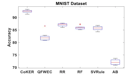
Fig. 4: Box plot of the mean classification accuracies of MNIST dataset across the five comparative methods
testing. Comparing CokER with five different methods namely Weighted Classifier Ensemble method based on Quadratic Forms (QFWEC), Ridge regression (RR), Random Forest (RF), Simple Vote Rule (SVRule) and Adaboost (AB) .
Fig. 4 shows the classification accuracy of the propose CoKER and the comparative methods on the MNIST dataset. The proposed method outperforms the rest of the comparative methods. More sig-nificantly, AB achieves the lowest classification accuracy perfor-mance than the rest of the comparative methods which also perform a poorly as compared to the propose CoKER.
5. CONCLUSION
In this paper, we investigated the problem of how to combine a set of kernel regressors into a unified ensemble regression framework. The framework can simultaneously couple multiple kernel regres-sors by minimizing total loss of ensembles in Reproducing Kernel Hilbert Space. In this way, one kernel regressor with more accurate fitting precession on data, can obtain bigger weight, which leads to a better overall ensemble performance. Experimental results on several UCI datasets for regression and classification, compared with several single models and ensemble models such as Gradient Boosting (GB), Tree Regression (TR), Support Vector Regression (SVR), Ridge Regression (RR) and Random Forest (RF), illustrate that, the proposed method achieves best performances among the comparative methods.
6. REFERENCES
[1] h49, author=Wornyo, Dickson Keddy and Shen, Xiang-Jun and Dong, Yong and Wang, Liangjun and Huang, Shu-Cheng, journal=World Wide Web, pages=1–18, year=2018, publisher=Springer.
[2] Xiangyu Chang, Shao-Bo Lin, and Ding-Xuan Zhou. Dis-tributed semi-supervised learning with kernel ridge regres-sion.Journal of Machine Learning Research, 18(46):1–22, 2017.
[3] Luefeng Chen, Mengtian Zhou, Min Wu, Jinhua She, Zhentao Liu, Fangyan Dong, and Kaoru Hirota. Three-layer weighted fuzzy support vector regression for emotional intention under-standing in human-robot interaction.IEEE Transactions on Fuzzy Systems, 2018.
[4] Kai Cheng and Zhenzhou Lu. Adaptive sparse polynomial chaos expansions for global sensitivity analysis based on sup-port vector regression.Computers & Structures, 194:86–96, 2018.
[5] R Dennis Cook and Liliana Forzani. Big data and partial least-squares prediction.Canadian Journal of Statistics, 46(1):62– 78, 2018.
[6] Kamalika Das and Ashok N Srivastava. Sparse inverse ker-nel gaussian process regression.Statistical Analysis and Data Mining: The ASA Data Science Journal, 6(3):205–220, 2013. [7] Harris Drucker, Christopher JC Burges, Linda Kaufman, Alex J Smola, and Vladimir Vapnik. Support vector regres-sion machines. InAdvances in neural information processing systems, pages 155–161, 1997.
[8] Charles W Edmunds, Choo Hamilton, Keonhee Kim, Nico-las Andre, and Nicole Labbe. Rapid detection of ash and organics in bioenergy feedstocks using fourier transform in-frared spectroscopy coupled with partial least-squares regres-sion.Energy & Fuels, 31(6):6080–6088, 2017.
[9] Siddharth Hariharan, Siddhesh Tirodkar, Alok Porwal, Avik Bhattacharya, and Aurore Joly. Random forest-based prospectivity modelling of greenfield terrains using sparse de-posit data: an example from the tanami region, western aus-tralia.Natural Resources Research, 26(4):489–507, 2017. [10] Md Al Mehedi Hasan, Mohammed Nasser, Biprodip Pal, and
Shamim Ahmad. Support vector machine and random forest modeling for intrusion detection system (ids).Journal of In-telligent Learning Systems and Applications, 6(01):45, 2014. [11] Justin Heinermann and Oliver Kramer. Precise wind power prediction with svm ensemble regression. In International Conference on Artificial Neural Networks, pages 797–804. Springer, 2014.
[12] Kristoffer H Hellton and Nils Lid Hjort. Fridge: Focused fine-tuning of ridge regression for personalized predictions. Statis-tics in medicine, 37(8):1290–1303, 2018.
[13] Masayuki Hirukawa and Artem Prokhorov. Consistent esti-mation of linear regression models using matched data. Jour-nal of Econometrics, 203(2):344–358, 2018.
[14] Achin Jain, Francesco Smarra, Madhur Behl, and Rahul Mangharam. Data-driven model predictive control with re-gression treesan application to building energy management. ACM Transactions on Cyber-Physical Systems, 2(1):4, 2018. [15] Aman Mohammad Kalteh. Monthly river flow forecasting us-ing artificial neural network and support vector regression models coupled with wavelet transform.Computers & Geo-sciences, 54:1–8, 2013.
[16] Zhen Lei and Stan Z Li. Coupled spectral regression for matching heterogeneous faces. InComputer Vision and Pat-tern Recognition, 2009. CVPR 2009. IEEE Conference on, pages 1123–1128. IEEE, 2009.
[17] Yantao Li, Hailong Hu, Gang Zhou, and Shaojiang Deng. Sensor-based continuous authentication using cost-effective kernel ridge regression.IEEE Access, 2018.
[18] Jiajun Liu, Shuo Shang, Kai Zheng, and Ji-Rong Wen. Multi-view ensemble learning for dementia diagnosis from neu-roimaging: an artificial neural network approach. Neurocom-puting, 195:112–116, 2016.
[19] Sujith Mangalathu, Jong-Su Jeon, and Reginald DesRoches. Critical uncertainty parameters influencing seismic perfor-mance of bridges using lasso regression. Earthquake Engi-neering & Structural Dynamics, 47(3):784–801, 2018. [20] Santosh Singh Rathore and Sandeep Kumar. A decision
soft-ware faults prediction.ACM SIGSOFT Software Engineering Notes, 41(1):1–6, 2016.
[21] Celine B Santiago, Jing-Yao Guo, and Matthew S Sig-man. Predictive and mechanistic multivariate linear regres-sion models for reaction development. Chemical science, 9(9):2398–2412, 2018.
[22] Bernhard Sch¨olkopf, Alexander J Smola, Francis Bach, et al. Learning with kernels: support vector machines, regulariza-tion, optimizaregulariza-tion, and beyond. MIT press, 2002.
[23] Ingo Steinwart, Don Hush, and Clint Scovel. An explicit de-scription of the reproducing kernel hilbert spaces of gaus-sian rbf kernels.IEEE Transactions on Information Theory, 52(10):4635–4643, 2006.
[24] Shengzheng Wang, Baoxian Ji, Jiansen Zhao, Wei Liu, and Tie Xu. Predicting ship fuel consumption based on lasso re-gression.Transportation Research Part D: Transport and En-vironment, 2017.
[25] Yaozheng Wang, Dawei Feng, Dongsheng Li, Xinyuan Chen, Yunxiang Zhao, and Xin Niu. A mobile recommendation sys-tem based on logistic regression and gradient boosting deci-sion trees. InIJCNN, pages 1896–1902, 2016.
[26] Hongyan Wu, Yunpeng Cai, Yongsheng Wu, Ren Zhong, Qi Li, Jing Zheng, Denan Lin, and Ye Li. Time series anal-ysis of weekly influenza-like illness rate using a one-year pe-riod of factors in random forest regression.Bioscience trends, 11(3):292–296, 2017.