Sensitivity Analysis for Optimal Distributed Generation Placement in Port Harcourt 33kv Power Distribution System

© 2019, IRJET | Impact Factor value: 7.34 | ISO 9001:2008 Certified Journal

| Page 1710

Sensitivity Analysis for Optimal Distributed Generation Placement in

Port Harcourt 33kv Power Distribution System

Engr. Chizindu Stanley Esobinenwu

_{, Engr. Dr. A.J. Atuchukwu}

_and

_{. Dr. J.P.ILoh}

1

_{Department of Electrical/Electronic Engineering, University of Port Harcourt, Rivers State, Nigeria.}

_{Department of Electrical/Electronic Engineering, Chukwuemeka Odumegwu Ojukwu University Uli,}

Anambra State.

---***---

Abstract: In this paper loss sensitivity factor method is used to identify the optimal placement of DG units in power distribution system. Simulations are conducted on 73-bus Port Harcourt 33 kV Power distribution system modelled in Electrical Transient Analyzer program (ETAP 12.6) software using Newton Raphson (N-R) load flow method. The results obtained showed that 35 load buses are outside the statutory voltage constraint limit (0. 95p.u – 1. 05p.u) that is 31.35KV- 34.65KV. Gas turbine synchronous generators (DGs) of 25MW are placed at the optimal position of the candidate buses identified by sensitivity analysis. To verify the efficacy of the proposed method, load flow analysis was repeated for the test system. The result obtained after DG placement reveals improvement in voltage profile and loss reduction.

Keywords: Distribution system, Loss sensitivity factor, Distributed Generation, load flow, Newton Raphson, ETAP.

1. INTRODUCTION

Loss sensitivity factor is the key method for the optimal DG placement in distribution system. It provides the sequence in which the candidate buses are to be considered for DG placement.

Distributed generation (DG) is a new trend that can be used to improve availability of power and reliability of the power network. Currently, there is no unified definition of distributed generation which is also known as embedded generation or dispersed generation or decentralised generation. In this paper, distributed generation (DG) implies the use of small, modular, decentralized, off- grid or grid connected generators spotted throughout a power system network, providing the electricity locally to load customers (Thomas et al., 2001). The recent literatures relating to optimal placement of DG using sensitivity analysis are:

Graham et al. (2000) applied loss sensitivity factor method (LSF) based on the principle of linearization of the original nonlinear equation (loss equation) around the initial operating point, which helps to reduce the amount of solution space. Optimal placement of DG units is determined exclusively for the various distributed load profiles to minimize the total losses. They iteratively increased the size of DG unit at all buses and then calculated the losses; based on loss calculation they ranked the nodes. Top ranked nodes are selected for DG unit placement

Kanth et al. (2013) implemented sensitivity analysis and PSO on standard IEEE 15 bus test system for determining the location and size of DG in the distribution networks in order to reduce the real power losses of the system. To include the presence of harmonics, PSO was integrated with a harmonic power flow algorithm (HPF).

Nalini et al. (2014) presented a heuristic optimization technique named particle swarm optimization (PSO) as a working tool to minimize simultaneously the economic cost of overall system by changing sitting and varying sizes of DGs. With respect to voltage profile THD and loss reduction by using the sensitivity analysis.

Lakshyabhat et al. (2015) presented sensitivity analysis for 14 bus systems in a distribution network with distributed generators. An analysis is carried out by selecting the most optimum location in placing the Distributed Generators through load flow analysis and seeing where the voltage profile rises. Matlab programming is used for simulation of voltage profile in the respective buses after introduction of DG’s. A tolerance limit of +/-5% of the base value has to be maintained. To maintain the tolerance limit, 3 methods are used. Sensitivity analysis of 3 methods for voltage control is carried out to determine the priority among the methods.

© 2019, IRJET | Impact Factor value: 7.34 | ISO 9001:2008 Certified Journal

| Page 1711

Divya et al. (2016) used sensitivity analysis to determine the location of DG and particle swarm optimization to determine the size of DG to minimize the power losses in the distribution network. The result, so obtained show the improvement of voltage profile, reduction of real power loss using MATLAB.

Kumar et al. (2018) presented loss sensitivity factor method to identify optimal placement of DGs to minimize the power losses and to improve voltage profile and reliability in distribution system. Methodology is applied to IEEE 33-bus Radial Distribution System and the obtained results are compared.

Suresh et al. (2018) proposed dragonfly algorithm to determine the optimal DG placement for benefit maximization in distribution networks and also compared with loss sensitivity factors for 33-bus system.

Newton Raphson Load flow programs compute the voltage magnitudes and phase angles at each bus of the network under steady state operating conditions. These programs also compute real and reactive power in each of the line and power losses for all equipment, including transformers and distribution lines; thus overloaded transformers and distribution lines are identified and remedial measures can be implemented. The software used for the analysis is ETAP 12.6 is a fully graphical Electrical Transient Analyzer Program that provides a very high level of reliability, protection and security of critical applications. Among ETAP’s most powerful features are the composite network and motor element. Composite elements allow you to graphically nest network elements within themselves to an arbitrary depth. For example, a composite network can contain other composite networks, providing the capability to construct complex electrical networks while still maintaining a clean, uncluttered diagram that you want to emphasize. ETAP provides five levels of error checking. The active error viewer appears when you attempt to run a study with missing or inappropriate data.

2. MATERIALS

The materials are: Distribution line data, bus data, load readings of the distribution feeders, installed capacity of

transmission substations, injection substations, power rating of distribution transformers connected to the injection substations and Port Harcourt 33kv power distribution network diagram.

Software’s ( MATLAB, ETAP).

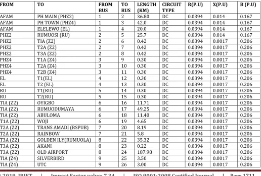
TABLE 1: LINE DATA FOR PORT HARCOURT POWER DISTRIBUTION NETWORK

FROM TO FROM

BUS TO BUS LENGTH (KM) CIRCUIT TYPE R(P.U) X(P.U) B (P.U)

AFAM PH MAIN (PHZ2) 1 2 36.80 DC 0.0394 0.014 0.167

AFAM PH TOWN (PHZ4) 1 3 42.0 DC 0.0394 0.014 0.167

AFAM ELELEWO (EL) 1 4 20.0 DC 0.0394 0.014 0.167

PHZ2 RUMUOSI (RU) 2 5 25.7 DC 0.0394 0.014 0.167

PHZ2 TIA (Z2) 2 6 0.42 DC 0.0394 0.0017 0.206

PHZ2 T2A (Z2) 2 7 0.42 DC 0.0394 0.0017 0.206

PHZ2 T3A (Z2) 2 8 0.42 DC 0.0394 0.0017 0.206

PHZ4 T1A (Z4) 3 9 0.30 DC 0.0394 0.0017 0.206

PHZ4 T2A (Z4) 3 10 0.30 DC 0.0394 0.0017 0.206

PHZ4 T2B (Z4) 3 11 0.30 DC 0.0394 0.0017 0.206

EL T1(EL) 4 12 0.30 DC 0.0394 0.0017 0.206

EL T2 (EL) 4 13 0.30 DC 0.0394 0.0017 0.206

RU T1(RU) 5 14 0.30 DC 0.0394 0.0017 0.206

RU T2(RU) 5 15 0.30 DC 0.0394 0.0017 0.206

TIA (Z2) OYIGBO 6 16 11.71 DC 0.0394 0.0017 0.206

TIA (Z2) RUMUODUMAYA 6 17 49.25 DC 0.0394 0.0017 0.206

TIA (Z2) ABULOMA 6 18 11.40 DC 0.0394 0.0017 0.206

T1A (Z2) WOJI 6 19 4.65 DC 0.0394 0.0017 0.206

T2A (Z2) TRANS AMADI (RSPUB) 7 20 8.19 DC 0.0394 0.0017 0.206

T2A (Z2) RAINBOW 7 21 5.8 DC 0.0394 0.0017 0.206

T3A (Z2) GOLDEN ILY(RUMUOLA) 8 22 35.32 DC 0.0394 0.0017 0.206

T3A (Z2) AKANI 8 23 0.22 DC 0.0394 0.0017 0.206

T3A (Z2) OLD AIRPORT 8 24 187.98 DC 0.0394 0.0017 0.206

TIA (Z4) SILVERBIRD 9 25 3.50 DC 0.0394 0.0017 0.206

© 2019, IRJET | Impact Factor value: 7.34 | ISO 9001:2008 Certified Journal

| Page 1712

T1A (Z4) BOLOKIRI 9 27 11.04 DC 0.0394 0.0017 0.206

TIA (Z4) RUMUOLUMENI 9 28 12.3 DC 0.0394 0.0017 0.206

T2A (Z4) UST 10 29 15.15 DC 0.0394 0.0017 0.206

T2B (Z4) SECRETARIAT 11 30 151.24 DC 0.0394 0.0017 0.206

T1(EL) ELEME 12 31 65.4 DC 0.0394 0.0017 0.206

TI(EL) IGBO ETCHE 12 32 9.0 DC 0.0394 0.0017 0.206

T1(EL) IRIEBE 12 33 70.0 DC 0.0394 0.0017 0.206

T2 (EL) BORI 13 34 60 DC 0.0394 0.0017 0.206

T2 (EL) RSTV(ELELEWO) 13 35 50.0 DC 0.0394 0.0017 0.206

T2 (EL) BRISTLE 13 36 20 DC 0.0394 0.0017 0.206

T1(RU) NEW AIRPORT 14 37 38 DC 0.0394 0.0017 0.206

T1 (RU) RUKPOKWU 14 38 15 DC 0.0394 0.0017 0.206

T2 (RU) NTA 15 39 5 DC 0.0394 0.0017 0.206

T2 (RU) UPTH 15 40 4.0 DC 0.0394 0.0017 0.206

OYIGBO FDR AWETO GUEST HOUSE 16 41 7.19 DC 0.0394 0.0017 0.206

OYIGBO FDR SHELL RES 16 42 8.5 DC 0.0394 0.0017 0.206

RUMUODUMA

YA FDR AGIP/ OKPORO 17 43 35.6 DC 0.0394 0.0017 0.206

RUMUODUMA

YA FDR UNIPORT 17 44 55.6 DC 0.0394 0.0017 0.206

RUMUODUMA

YA FDR CHOBA 17 45 55.6 DC 0.0394 0.0017 0.206

ABULOMA

FDR STALLION PHASE 2 18 46 2.0 DC 0.0394 0.0017 0.206

ABULOMA

FDR GULF ESTATE 18 47 5.0 DC 0.0394 0.0017 0.206

TRANS AMADI

(RSPUB) FDR FIRST ALLUMINIUM 20 48 2.46 DC 0.0394 0.0017 0.206

TRANS AMADI

(RSPUB) FDR ELF NIG 20 49 4.1 DC 0.0394 0.0017 0.206

TRANS AMADI

(RSPUB) FDR BEKEMS PROPERTY 20 50 5.8 DC 0.0394 0.0017 0.206

TRANS AMADI

(RSPUB) FDR TRANS AMADI GARDENS 20 51 8.19 DC 0.0394 0.0017 0.206

TRANS AMADI

(RSPUB) FDR GALBA 20 52 60 DC 0.0394 0.0017 0.206

TRANS AMADI

(RSPUB) FDR RIVOC 20 53 5.8 DC 0.0394 0.0017 0.206

TRANS AMADI

(RSPUB) FDR AIR LIQUID 20 54 8.19 DC 0.0394 0.0017 0.206

TRANS AMADI

(RSPUB) FDR STALLION 1 20 55 6.2 DC 0.0394 0.0017 0.206

TRANS AMADI

(RSPUB) FDR OIL INDUSTRY 20 56 7.0 DC 0.0394 0.0017 0.206

TRANS AMADI

(RSPUB) FDR ONWARD FISHERY 20 57 9.70 DC 0.0394 0.0017 0.206

RAINBOW

FDR ELEKAHIA 21 58 7.0 DC 0.0394 0.0017 0.206

RUMUOLA

FDR SHELL. INDUSTRIAL 22 59 5.2 DC 0.0394 0.0017 0.206

RUMUOLA

FDR PRESIDENTIAL HOTEL 22 60 21.0 DC 0.0394 0.0017 0.206

OLD AIRPORT

FDR ENEKA 24 61 30.0 DC 0.0394 0.0017 0.206

OLD AIRPORT

FDR BIG TREAT 24 62 35.0 DC 0.0394 0.0017 0.206

© 2019, IRJET | Impact Factor value: 7.34 | ISO 9001:2008 Certified Journal

| Page 1713

UTC FDR WATER WORKS 26 64 6.0 DC 0.0394 0.0017 0.206

BOLOKIRI

FDR EASTERN BYPASS 27 65 9.0 DC 0.0394 0.0017 0.206

RUMUOLUME

NI FDR SCHOOL OF NURSING 28 66 29.5 DC 0.0394 0.0017 0.206

RUMUOLUME

NI FDR U.O.E 28 67 20.5 DC 0.0394 0.0017 0.206

RUMUOLUME

NI FDR NAVAL BASE 28 68 32.8 DC 0.0394 0.0017 0.206

RUMUOLUME

NI FDR MASTER ENERGY 28 69 4.3 DC 0.0394 0.0017 0.206

UST AGIP HOUSING ESTATE 29 70 5.0 DC 0.0394 0.0017 0.206

UST NAOC AGIP BASE 29 71 3.2 DC 0.0394 0.0017 0.206

SECRETARIAT JUANUTA 30 72 35.6 DC 0.0394 0.0017 0.206

SECRETARIAT MARINE BASE 30 73 7.0 DC 0.0394 0.0017 0.206

Source: Port Harcourt electricity distribution company (PHEDC)

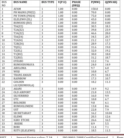
TABLE 2: DATA FOR 73- BUS PORT HARCOURT POWER DISTRIBUTION SYSTEM

BUS

NO BUS NAME BUS TYPE V(P.U) PHASE (DEQ) P(MW) Q(MVAR)

1 AFAM 1 1.00 0.00 150.0 0.00

2 PH MAINS (PHZ2) 2 1.00 0.00 70.0 0.00

3 PH TOWN (PHZ4) 2 1.00 0.00 75.0 0.00

4 ELELEWO (EL) 2 1.00 0.00 45.0 0.00

5 RUMUOSI (RU) 2 1.00 0.00 30.0 0.00

6 TIA(Z2) 3 0.00 0.00 30.5 18.3

7 T2A(Z2) 3 0.00 0.00 39.8 23.9

8 T3A(Z2) 3 0.00 0.00 46.6 28.0

9 TIA(Z4) 3 0.00 0.00 34.5 20.7

10 T2AZ4) 3 0.00 0.00 21.2 12.7

11 T2B(Z4) 3 0.00 0.00 28.9 17.3

12 TI(EL) 3 0.00 0.00 31.6 19.0

13 T2(EL) 3 0.00 0.00 32.0 19.2

14 T1(RU) 3 0.00 0.00 30.0 18.0

15 T2(RU) 3 0.00 0.00 31.2 18.7

16 OYIGBO 3 0.00 0.00 12.2 7.6

17 RUMUODUMAYA 3 0.00 0.00 24.0 14.9

18 ABULOMA 3 0.00 0.00 9.7 6.0

19 WOJI 3 0.00 0.00 10.8 6.7

20 TRANS AMADI 3 0.00 0.00 29.5 18.3

21 RAINBOW 3 0.00 0.00 17.3 10.7

22 GOLDEN

LILY(RUMUOLA) 3 0.00 0.00 18.2 11.3

23 AKANI 3 0.00 0.00 14.9 9.2

24 OLD AIRPORT 3 0.00 0.00 21.8 13.5

25 SILVERBIRD 3 0.00 0.00 16.0 9.9

26 UTC 3 0.00 0.00 10.8 6.7

27 BOLOKIRI 3 0.00 0.00 9.8 6.1

28 RUMUOLUMENI 3 0.00 0.00 13.8 8.6

29 UST 3 0.00 0.00 22.8 7.9

30 SECRETARIAT 3 0.00 0.00 16.2 10.04

31 ELEME 3 0.00 0.00 20.3 12.6

32 IGBO ETCHE 3 0.00 0.00 26.6 16.5

33 IRIEBE 3 0.00 0.00 8.9 5.5

34 BORI 3 0.00 0.00 11.4 7.1

© 2019, IRJET | Impact Factor value: 7.34 | ISO 9001:2008 Certified Journal

| Page 1714

36 BRISTLE 3 0.00 0.00 10.8 6.7

37 NEW AIRPORT 3 0.00 0.00 20.9 13.0

38 RUKPOKWU 3 0.00 0.00 12.1 7.5

39 NTA 3 0.00 0.00 18.0 11.2

40 UPTH 3 0.00 0.00 13.6 8.4

41 AWETOGUEST

HOUSE 3 0.00 0.00 10.1 6.3

42 SHELL RES 3 0.00 0.00 12.4 7.7

43 AGPIP/ OKPORO 3 0.00 0.00 11.2 6.9

44 UNIPORT 3 0.00 0.00 10.0 6.2

45 CHOBA 3 0.00 0.00 6.5 4.0

46 STALLION PHASE 2 3 0.00 0.00 8.9 5.5

47 GULF ESTATE 3 0.00 0.00 7.4 4.6

48 FIRST

ALLUMINIUM 3 0.00 0.00 10.6 6.6

49 ELF NIG 3 0.00 0.00 12.0 7.4

50 BEKEMS PROPERTY 3 0.00 0.00 10.5 6.5

51 TRANS AMADI

GARDENS 3 0.00 0.00 11.4 7.1

52 GALBA 3 0.00 0.00 10.9 6.8

53 RIVOC 3 0.00 0.00 12.3 7.6

54 AIR LIQUID 3 0.00 0.00 10.5 6.5

55 STALLION 1 3 0.00 0.00 13.4 8.3

56 OIL INDUSTRY 3 0.00 0.00 12.2 7.6

57 ONWARD FISHERY 3 0.00 0.00 13.8 8.6

58 ELEKAHIA 3 0.00 0.00 14.8 9.2

59 SHELL. INDUSTRIAL 3 0.00 0.00 13.8 8.6

60 PRESIDENTIAL

HOTEL 3 0.00 0.00 10.7 6.6

61 ENEKA 3 0.00 0.00 7.9 4.9

62 BIG TREAT 3 0.00 0.00 8.7 5.4

63 SHELL KIDNEY

ISLAND 3 0.00 0.00 5.2 3.3

64 WATER WORKS 3 0.00 0.00 3.8 2.4

65 EASTERN BYPASS 3 0.00 0.00 11.6 7.2

66 SCHOOL OF

NURSING 3 0.00 0.00 3.7 2.3

67 U.O.E 3 0.00 0.00 13.2 8.2

68 NAVAL BASE 3 0.00 0.00 10.1 6.3

69 MASTER ENERGY 3 0.00 0.00 7.9 4.9

70 AGIP HOUSING

ESTATE 3 0.00 0.00 8.8 5.5

71 NAOC AGIP BASE 3 0.00 0.00 9.8 6.1

72 JUANUTA 3 0.00 0.00 11.0 6.8

73 MARINE BASE 3 0.00 0.00 8.7 5.4

Source: Port Harcourt Electricity Distribution Company (PHEDC)

Key: 1 (Slack bus)

2 (PV bus)

© 2019, IRJET | Impact Factor value: 7.34 | ISO 9001:2008 Certified Journal

| Page 1715

3 METHODOLOGY

The methodology adopted are:

i. Modelling of 73 bus network of 33kV Port-Harcourt power Distribution Network using Electrical Transient

Analyzer Program (ETAP 12.6) software for load flow analysis.

ii. Steady state assessment of the network through load flow Analysis using Newton-Raphson (N-R) method.

iii. Loss sensitivity factor method.

Newton Raphson load flow will be simulated in ETAP software. This will be used to come up with the candidate buses for DG placement using loss sensitivity factor method.

3.1 COMPUTATIONAL PROCEDURE FOR NEWTON-RAPHSON METHOD

The computational procedure for Newton-Raphson method using polar coordinate is as follows:

1. Form Ybus.

2. Assume initial values of bus voltages / Vi /0 and phase angles °i for i = 2, 3, … n for load buses and phase angles for

PV buses. Normally we set the assumed bus voltage magnitude and its phase angle equal to slack bus quantities / V1 / = 1.0, = 0o_.

3. Compute Pi and Qi for each load bus from the following equations:

Pi =



 n

i k

Vi Vk Yik cos ( … ……….. (3.1.1)

Qi =



 n

i k

ViVk Yik sin ( ………(3.1.2)

4. Compute the scheduled error and Qi for each load bus from the following relations.

Pi

i

r

)

(

= Pi sp - P

)

(

)

(

cal

i

r

i = 2,3,…n ………. (3.1.3)

Qi

i

r

)

(

= Qi sp - Q

)

(

)

(

cal

i

r

i = 2,3,…n ……….(3.1.4)

For PV buses, the exact value of Qi is not specified, but its limits are known. If the calculated value of Qi is beyond the

limits, then an appropriate limit is imposed and Qi is also calculated by subtracting the calculated value of Qi from the

appropriate limit. The bus under consideration is now treated as a load (PQ) bus.

5. Compute the elements of the Jacobian matrix

Using the estimated I Vi I and from step 2

6. Obtain and / Vi / from equation

© 2019, IRJET | Impact Factor value: 7.34 | ISO 9001:2008 Certified Journal

| Page 1716

7. Using the value of and I Vi I calculated in step 6, modify the voltage magnitude and phase angle at all load buses

by the equations

/ Vi(r+1) /= I/Vi(r) / + I/Vi(r) /………. (3.1.6)

i(r+1) = i(r) + i(r) ………(3.1.7)

Start the next iteration cycle at step 2 with these modified / Vi / and

8. Continue until scheduled errors Pi(r) and Qi(r) for all load buses are within a specified tolerance, that is,

Pi(r)< Qi(r) <

Where denotes the tolerance level for load buses.

9. Calculate line flows and power at the slack bus exactly in the same manner as in the GS method.

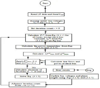
The flowchart for Newton-Raphson method using polar coordinates for load flow solution is given in Fig. 3.1

Fig. 3.1. Flowchart for load flow solution using NR method in polar coordinates.

3.2 SENSITIVITY ANALYSIS FOR OPTIMAL PLACEMENT OF DISTRIBUTED GENERATION

Loss sensitivity factor method (LSF) is applied to Port Harcourt power distribution network to determine the candidate

© 2019, IRJET | Impact Factor value: 7.34 | ISO 9001:2008 Certified Journal

| Page 1717

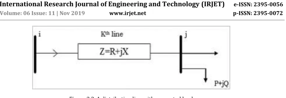
Figure 3.2. A distribution line with connected load

Considering a distribution link shown in figure 3.2. The link represents a distribution line connecting two buses, and j of Port Harcourt distribution system. The magnitude of the two bus voltages, vi and vj are known by load flow study. The real and reactive power losses in each of the line and power flow are obtained by load flow studies.

The real power loss in distribution line can be expressed as

(3.1.8)

(3.85)

Similarly, reactive power loss in the distribution line can be expressed as

(3.1.9)

LSF value can be expressed by derivative of the equations (3.1.8)

(3.1.10)

(3.1.11)

Loss sensitivity for all the candidate buses will be calculated using equation (3.1.11).

Few topmost load ranked buses will be selected for optimal DG placement in the test system. Synchronous generator based DGs will be placed on this bus and the load flow analysis repeated on the entire system to determine the voltage profile and the system losses.

4. SIMULATION RESULTS AND DISCUSSION

Table 4.1: LOSS SENSITIVITY FACTORS FOR 35 BUS SYSTEM

(Source: Calculated Result)

Bus No Pi (pu) R(pu) Vi (pu) LSF LSF Ranking

BUS 7 0.398 0.857 0.914 0.817 22

BUS 9 0.345 0.612 0.919 0.500 25

BUS 16 0.102 0.612 0.914 0.149 32

BUS 20 0.216 0.612 0.856 0.361 27

BUS 21 0.122 0.612 0.841 0.211 28

BUS 25 0.128 0.612 0.894 0.196 29

© 2019, IRJET | Impact Factor value: 7.34 | ISO 9001:2008 Certified Journal

| Page 1718

BUS 27 0.081 0.612 0.909 0.120 35

BUS 28 0.097 0.612 0.837 0.169 30

BUS 31 0.102 8.568 0.947 1.949 7

BUS 37 0.216 11.424 0.929 5.718 1

BUS 39 0.122 0.612 0.946 0.167 31

BUS 41 0.128 4.080 0.904 1.278 13

BUS 42 0.216 2.856 0.854 1.692 8

BUS 44 0.081 2.448 0.948 0.441 26

BUS 48 0.097 4.896 0.851 1.312 11

BUS 49 0.102 2.244 0.855 0.626 23

BUS 50 0.089 7.140 0.954 1.396 10

BUS 51 0.122 2.448 0.854 0.819 21

BUS 52 0.128 2.448 0.855 0.857 19

BUS 53 0.089 6.324 0.846 1.573 9

BUS 54 0.081 4.488 0.851 1.004 15

BUS 55 0.097 2.244 0.854 0.597 24

BUS 56 0.102 4.080 0.851 1.149 14

BUS 57 0.216 6.324 0.845 3.826 3

BUS 58 0.122 6.528 0.833 2.296 6

BUS 59 0.128 10.608 0.944 3.047 4

BUS 63 0.089 0.612 0.895 0.136 33

BUS 64 0.081 4.284 0.909 0.840 20

BUS 65 0.097 4.080 0.894 0.990 17

BUS 66 0.102 3.060 0.837 0.891 18

BUS 67 0.216 8.160 0.83 5.117 2

BUS 68 0.122 2.856 0.834 1.002 16

BUS 69 0.128 6.528 0.835 2.397 5

BUS 71 0.089 6.528 0.949 1.290 12

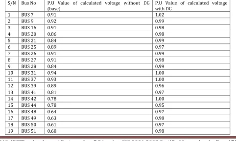
Table 4.2: Load flow Comparative results of the candidate bus Voltage Magnitude Before and After DG Placement (source: Simulation result)

S/N Bus No P.U Value of calculated voltage without DG

(base) P.U Value of calculated voltage with DG

1 BUS 7 0.91 1.02

2 BUS 9 0.92 0.99

3 BUS 16 0.91 0.98

4 BUS 20 0.86 0.98

5 BUS 21 0.84 0.99

6 BUS 25 0.89 0.97

7 BUS 26 0.91 0.99

8 BUS 27 0.91 0.98

9 BUS 28 0.84 0.99

10 BUS 31 0.94 1.00

11 BUS 37 0.93 1.00

12 BUS 39 0.89 0.96

13 BUS 41 0.81 0.97

14 BUS 42 0.78 1.00

15 BUS 44 0.78 0.95

16 BUS 48 0.64 0.97

17 BUS 49 0.63 0.98

18 BUS 50 0.61 0.97

© 2019, IRJET | Impact Factor value: 7.34 | ISO 9001:2008 Certified Journal

| Page 1719

20 BUS 52 0.59 0.98

21 BUS 53 0.57 1.00

22 BUS 54 0.56 0.97

23 BUS 55 0.55 0.97

24 BUS 56 0.54 0.97

25 BUS 57 0.53 1.00

26 BUS 58 0.51 1.00

27 BUS 59 0.57 1.00

28 BUS 63 0.50 0.97

29 BUS 64 0.50 0.98

30 BUS 65 0.48 0.97

31 BUS 66 0.45 0.99

32 BUS 67 0.43 1.00

33 BUS 68 0.43 0.99

34 BUS 69 0.42 1.00

35 BUS 71 0.47 0.95

22 25

32

2728 29

3435

30

7

1 31

13

8 26

11 23

10 21

19

9 15

24

14

3 6

4 33

20

1718

2 16

5 12

7 9 16 20 21 25 26 27 28 31 37 39 41 42 44 48 49 50 51 52 53 54 55 56 57 58 59 63 64 65 66 67 68 69 71

LS

F

R

an

ki

n

g

Bus No

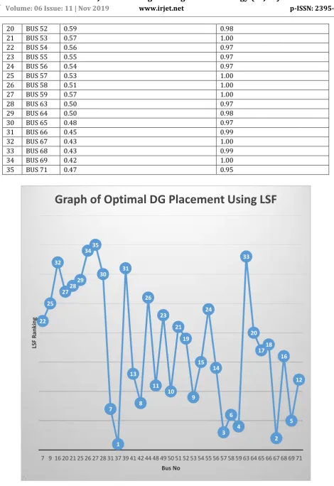
Graph of Optimal DG Placement Using LSF

© 2019, IRJET | Impact Factor value: 7.34 | ISO 9001:2008 Certified Journal

| Page 1720

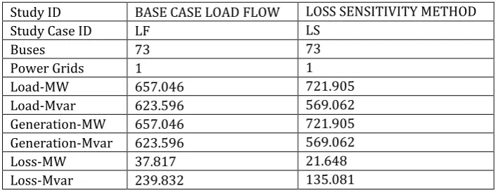
TABLE 4.3: SUMMARY OF RESULT BETWEEN BASE CASE LOAD FLOW AND LOSS SENSITIVITY FACTOR METHOD

Study ID BASE CASE LOAD FLOW LOSS SENSITIVITY METHOD

Study Case ID LF LS

Buses 73 73

Power Grids 1 1

Load-MW 657.046 721.905

Load-Mvar 623.596 569.062

Generation-MW 657.046 721.905

Generation-Mvar 623.596 569.062

Loss-MW 37.817 21.648

Loss-Mvar 239.832 135.081

5. DISCUSSION

After performing the load flow analysis of the 73-bus test distribution system under review using ETAP12.6 software, an alert summary report was generated which shows 35 candidate load bus are outside the statutory voltage constraint limit (0. 95p.u – 1. 05p.u) that is 31.35KV- 34.65KV.

Loss sensitivity factor was performed on all the candidate buses. The findings on the obtained ranking demonstrate that few topmost load buses were appropriate for the placement of DGs as shown in fig.4.1. The candidate buses identified are: BUS 31, BUS37, BUS42, BUS53, BUS57, BUS58, BUS59, BUS67, BUS 69. Distributed generation units of 25MW gas turbine synchronous generator (DG1-9 units) were placed at these buses and load flow simulation repeated. The results are showed in table 4.2 with improvement in voltage profile and reduction of power losses in the distribution lines.

6. CONCLUSION

The loss sensitivity factor method is useful in reducing the search space for optimal DG placement and particle swarm optimization. One consideration in determining the best placement for DG is its effect on losses and voltage profile. When the DGs were optimally placed at the candidate buses identified by loss sensitivity factor, there was an acceptable improvement in the entire distribution network in terms of loss minimization and voltage profile enhancement.

Distributed generation (DG) is a new trend that can be used to improve availability of power and reliability of the power network.

7. REFERNCES

1. Divya,C.,& Manohar,T.G.(2016).Optimal location of DG units using sensitivity analysis. International Journal of

Advanced Technology and Innovative Research, Vol.8, No. 21, pp.4192-4196.

2. Graham,W., James, A., & Mc-Donald, R. (2000).Optimal placement of distributed generation sources in power

systems, IEEE Trans. Power Sys., Vol.19, No.5, pp.127- 134.

3. Kumar,G.S., Sarat,S.K.,&Jayaram,K.S.V.K.(2018).DG placement using loss sensitivity factor method for loss

reduction and reliability improvement in distribution system. International Journal of Engineering & Technology, Vol.74, No.4, pp.236-240.

4. Kanth, D.S.K., Lalita, M.P., & Babu, P.S. (2013). Siting & sizing of Dg for power loss & Thd reduction, voltage improvement using Pso & sensitivity analysis. International journal of Engineering research and development, Vol.9, No.6, pp.1-7.

5. LakshyaBhat., Anubhav, S., & Shivarudraswamy (2015). Sensitivity Analysis for 14 Bus Systems in a Distribution

Network with Distributed Generators. Journal of Electrical and Electronics Engineering, Vol.10, No.3, pp.21-27.

6. Nalini, P., & Selvi.K.(2014). Power Quality improvement of distribution system by optimal placement of

© 2019, IRJET | Impact Factor value: 7.34 | ISO 9001:2008 Certified Journal

| Page 1721

7. Singh, N., Ghosh,S.,& Murari, K.(2015).Optimal sizing and placement of DG in radial Distribution Network using

Sensitivity based Methods, Vol.6, No.1, pp.1727-1734.

8. Suresh, M.C.V., & Belwin, E.J. (2018). Optimal DG placement for benefit maximization in distribution networks by

using Dragonfly algorithm. Suresh and Belwin Renewable, Vol.5, No.4, pp.1-8.

9. Thomas, A., Goran, A., & Lennart, S. (2001). Distributed generation: a definition. Electric Power Systems Research,