Quenching or Bursting:the Role of Stellar Mass, Environment, and Specific Star Formation Rate to z ~ 1

arXiv:submit/2121206 [astro-ph.GA] 4 Jan 2018

Preprint typeset using LA_{TEX style emulateapj v. 12/16/11}

QUENCHING OR BURSTING: THE ROLE OF STELLAR MASS, ENVIRONMENT, AND SPECIFIC STAR FORMATION RATE TOz∼1

Behnam Darvish1, Christopher Martin1, Thiago S. Gonc¸alves2, Bahram Mobasher3, Nick Z. Scoville1, and David Sobral4,5

Accepted for publication in the ApJ

ABSTRACT

Using a novel approach, we study the quenching and bursting of galaxies as a function of stellar mass (M∗), local environment (Σ), and specific star-formation rate (sSFR) using a large spectroscopic

sample of ∼ 123,000 GALEX/SDSS and ∼ 420 GALEX/COSMOS/LEGA-C galaxies to z ∼ 1. We show that out to z ∼1 and at fixed sSFR and local density, on average, less massive galaxies are quenching, whereas more massive systems are bursting, with a quenching/bursting transition at log(M∗/M⊙) ∼ 10.5-11 and likely a short quenching/bursting timescale (. 300 Myr). We find

that much of the bursting of star-formation happens in massive (log(M∗/M⊙) & 11), high sSFR

galaxies (log(sSFR/Gyr−1_{)&-2), particularly those in the field (log(Σ/Mpc}−2_{).0; and among group}

galaxies, satellites more than centrals). Most of the quenching of star-formation happens in low-mass (log(M∗/M⊙).9), low sSFR galaxies (log(sSFR/Gyr−1).-2), in particular those located in dense

environments (log(Σ/Mpc−2)&1), indicating the combined effects ofM∗and Σ in quenching/bursting

of galaxies sincez ∼1. However, we find that stellar mass has stronger effects than environment on recent quenching/bursting of galaxies toz∼1. At any givenM∗, sSFR, and environment, centrals are

quenchier (quenching faster) than satellites in an average sense. We also find evidence for the strength of mass and environmental quenching being stronger at higher redshift. Our preliminary results have potential implications for the physics of quenching/bursting in galaxies across cosmic time.

Subject headings: galaxies: evolution — galaxies: groups: general — galaxies: star formation — galaxies: high-redshift — ultraviolet: galaxies — large-scale structure of universe

1. _INTRODUCTION

What causes galaxies to stop forming stars — to quench — is still an unsolved problem in studies of galaxy formation and evolution. Several exter-nal and interexter-nal mechanisms with different quench-ing timescales have been proposed such as ram pres-sure stripping, viscous stripping, thermal evaporation, strangulation, galaxy-galaxy interactions, galaxy ha-rassment, mergers, galaxy-cluster tidal interactions (see the review by Boselli & Gavazzi 2006), halo quenching (Birnboim & Dekel 2003), AGN feedback (see the review by Fabian 2012), stellar feedback (Hopkins et al. 2014), and morphological quenching and secular processes (Sheth et al. 2005; Martig et al. 2009; Fang et al. 2013; Bluck et al. 2014; Nogueira-Cavalcante et al. 2018).

These processes might temporarily enhance star-formation in galaxies prior to quenching, or they can cause both negative (quenching) and positive (bursting) feedback. For example, compression of the gas due to thermal instability and turbulent motions and/or the in-flow of gas to the center can elevate star-formation in

1_{Cahill Center for Astrophysics, California Institute of}

Tech-nology, 1216 East California Boulevard, Pasadena, CA 91125, USA; email: [email protected]

2_{Observatorio do Valongo, Universidade Federal do Rio de}

Janeiro, Ladeira Pedro Antonio, 43, Saude, Rio de Janeiro-RJ 20080-090, Brazil

3_{University of California, Riverside, 900 University Ave,}

Riverside, CA 92521, USA

4_{Department of Physics, Lancaster University, Lancaster,}

LA1 4YB, UK

5_{Leiden Observatory, Leiden University, P.O. Box 9513,}

NL-2300 RA Leiden, The Netherlands

galaxies being stripped as a result of ram pressure, prior to the full interstellar medium (ISM) removal of galax-ies and hence subsequent quenching (Bekki & Couch 2003; Poggianti et al. 2016, 2017). Galaxy-galaxy in-teractions might cause the gas in the periphery of the interacting systems to get compressed and funnel to-wards the center, triggering a starburst and/or reviving nuclear activity (Mihos et al. 1992; Mihos & Hernquist 1996; Kewley et al. 2006; Ellison et al. 2008, 2013; Sobral et al. 2015; Stroe et al. 2015). AGN feedback can both reduce/stop star-formation through quasar-and radio-mode feedback (Best et al. 2005; Croton et al. 2006; Somerville et al. 2008; Hopkins & Elvis 2010; G¨urkan et al. 2015) and also trigger star-formation by compressing gas (by generating cool, dense cav-ities in the cocoon around the AGN jet; see e.g.; Silk & Nusser 2010; Gaibler et al. 2012; Wagner et al. 2012; Kalfountzou et al. 2017).

These processes are directly or indirectly associated with the “environment” or “stellar mass” of galax-ies and they often work together in the quench-ing mechanism (Peng et al. 2010; Quadri et al. 2012; Lee et al. 2015; Darvish et al. 2016; Henriques et al. 2017; Nantais et al. 2017; Kawinwanichakij et al. 2017; Guo et al. 2017; Smethurst et al. 2017). The gen-eral picture is that the “environmental quenching” be-comes important at later times (e.g.; Peng et al. 2010; Darvish et al. 2016; Hatfield & Jarvis 2017), particularly for less-massive galaxies (Peng et al. 2010; Quadri et al. 2012; Lee et al. 2015) and “mass quenching” is more ef-fective on more massive galaxies especially at higher red-shifts (Peng et al. 2010; Lee et al. 2015; Darvish et al. 2016). In groups, the environmental quenching is thought to be mostly associated with satellites, whereas mass quenching is mainly linked to centrals (Peng et al. 2012; Kovaˇc et al. 2014; Darvish et al. 2017). However, there are also inconsistencies in the literature on this topic. For example, although some studies point toward an independence of mass quenching and environmen-tal quenching processes (Peng et al. 2010; Quadri et al. 2012; Kovaˇc et al. 2014), others find that they depend on each other (Darvish et al. 2016; Kawinwanichakij et al. 2017). Despite recent progress, the relative importance of environmental and mass quenching, their evolution with cosmic time, and their influence on the physical properties of galaxies are still not fully understood.

In addition to stellar mass and the environment, an-other parameter that is strongly linked to galaxy quench-ing is the specific star-formation rate (sSFR; SFR/M∗).

The inverse of sSFR is a measure of how long it takes a galaxy to assemble its mass given its current SFR. There-fore, it is used to separate star-forming and quiescent sys-tems with the separating sSFR of ≈10−1_-10−2 _Gyr−1_.

The sSFR is tightly coupled toM∗for both star-forming

and quiescent systems over a broad redshift range (Noeske et al. 2007; Wuyts et al. 2011; Whitaker et al. 2012; Speagle et al. 2014; Shivaei et al. 2015). The sSFR also depends on the environment and on average, it is lower in denser regions, particularly at lower redshifts (Peng et al. 2010; Sobral et al. 2011; Scoville et al. 2013; Darvish et al. 2016; Hatfield & Jarvis 2017). However, the cause of lower sSFR in denser environments is still debatable, with some studies attributing this to only a lower fraction of star-forming galaxies in denser re-gions (Patel et al. 2009; Peng et al. 2010; Koyama et al. 2013; Darvish et al. 2014, 2015a, 2016; Hung et al. 2016; Duivenvoorden et al. 2016; Berti et al. 2017), whereas others linking it to both a lower fraction and a lower SFR of star-forming galaxies in denser environments than the field (Vulcani et al. 2010; Patel et al. 2011; Haines et al. 2013; Erfanianfar et al. 2016; Darvish et al. 2017). Nonetheless, the latter studies often find a small reduction of ∼0.1-0.3 dex in star-formation activity of star-forming galaxies in denser regions.

In this paper, we investigate both “quenching” and “bursting” of the overall galaxy population, satellite galaxies and centrals as a function of four main param-eters: stellar mass, sSFR, local environment, and red-shift sincez∼1, based on the recent methodology devel-oped by Martin et al. (2017). In Section 2, we introduce the data. Methods used to quantify the environment, quenching/bursting of galaxies and their properties are

developed in Section 3. The results are presented in Sec-tion 4, discussed in SecSec-tion 5, and summarized in SecSec-tion 6.

Throughout this study, we assume a flat ΛCDM cos-mology with H0=70 km s−1 Mpc−1, Ωm=0.3, and

ΩΛ=0.7 and a Salpeter initial mass function (IMF;

Salpeter 1955). As presented in Section 3.3, we define the Star Formation Acceleration (SFA) in units of mag Gyr−1 _as d(N UV−i)0

dt where dt is the past 300 Myr and (N U V −i)0 is the extinction-corrected N U V −i color

and the Star Formation Jerk (SFJ) as d(N UV_dt−i)0 where dt is the past 600-300 Myr. A positive (negative) SFA and SFJ indicate recent quenching (bursting). The SFA (SFJ) uncertainties are estimated as σ/√N, where σ is 1.4826×the median absolute deviation of the SFA (SFJ) andN is the number of data points.

2. _{DATA AND SAMPLE SELECTION}

2.1. Local Universe Sample (SDSS)

The local universe data are from the SDSS DR12 (Alam et al. 2015). Following Baldry et al. (2006), we select galaxies with clean Galactic-extinction-corrected Petrosian magnitude of r617.7 (after excluding stars), clean spectra (after removing duplicates) in the spec-troscopic redshift range of 0.02 6 z 6 0.12, located in the contiguous northern galactic cap (130.06RA (deg) 6 240.0 and 0.0 6 Dec (deg) 6 60.0). We use this sample (Sample A) for environmental measure estima-tions as it provides a contiguous field with relatively uniform, large spectroscopic coverage and completeness. Our estimation of galaxy properties requires SDSS and

GALEX photometry (Martin et al. 2005), 4000 ˚A break (Dn(4000)) and Hδ absorption-line index 6 _{(see Section}

3.3). Therefore, we match sample A with the GALEX

All-Sky Survey Source Catalog (GASC; Seibert et al. 2012) (matching radius of 5′′_{) and the resulting}

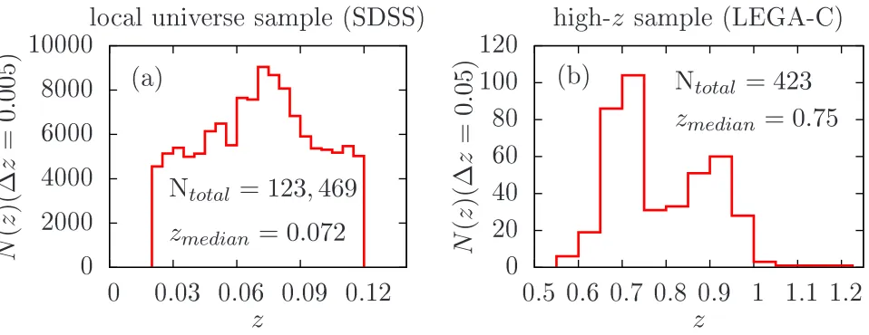
cat-alog is later matched with the MPA-JHU DR8 cata-log (Kauffmann et al. 2003) to retrieve reliable Dn(4000) and Hδ (median signal-to-noise (S/N) per pixel > 3) The k-correction recipe of Chilingarian et al. (2010) and Chilingarian & Zolotukhin (2012) is used to estimate the rest-frame colors and magnitudes. The final sample com-prises 123,469 sources. Figure 1 (a) shows the redshift distribution of sources. We use this final local-universe sample for scientific analysis (Section 4).

The magnitude cut of r 6 17.7 results in a redshift-dependent stellar mass completeness limit. We estimate the mass completeness limit using Pozzetti et al. (2010). We assign a limiting mass to each galaxy that corre-sponds to the stellar mass the galaxy would have if its ap-parent magnitude were the same as the magnitude limit of the sample (r617.7) At each redshift, the 90% mass completeness, for instance, is then defined as the stellar mass for which 90% of galaxies have their limiting mass below it. We use this 90% cut and estimate the com-pleteness limit to be log(M∗comp/M⊙)∼10.3 toz=0.12.

2.2. _{High Redshift Sample (LEGA-C)}

0 2000 4000 6000 8000 10000

0 0.03 0.06 0.09 0.12

N

(

z

)(

∆

z

=

0

.

00

5)

z

loal universe sample (SDSS)

0 20 40 60 80 100 120

0.5 0.6 0.7 0.8 0.9 1 1.1 1.2

N

(

z

)(

∆

z

=

0

.

05

)

z

high-

z

(a)

Ntotal

= 123

,

469

z

= 0

.

072

(b)

Ntotal

= 423

z

= 0

.

75

Fig. 1.—(a) Spectroscopic redshift distribution (in bins of ∆z=0.005) of our local-universe SDSS sample. (b) Spectroscopic redshift distribution (in bins of ∆z=0.05) of our high-zLEGA-C sample.

As we already mentioned, we require high signal-to-noise Dn(4000) and Hδ absorption features (along with photometric information) to robustly extract galaxy properties. At higher redshifts, the only such large and deep galaxy sample available so far is from the VLT LEGA-C spectroscopic survey (van der Wel et al. 2016) in the COSMOS field (Scoville et al. 2007) at z ≈ 0.6-1.0. Similar to the SDSS quality, this survey is designed to obtain high resolution (R ∼2500), high S/N (& 10, through 20 hour integration) continuum spectra in the wavelength range of∼6300-8800 ˚A for a large (∼3200) sample of galaxies at z ∼1 using the VIMOS spectro-graph. Their primary sample is K-band selected with a redshift-dependent magnitude limit to guarantee the coverage of the full galaxy types including quiescent, star-forming, and dusty systems at log(M∗/M⊙) & 10

(Chabrier IMF).

We use the LEGA-C first data release (892 spectra) by selecting galaxies with continuum S/N > 3 (typi-cal S/N> 10) and available Dn(4000) and Hδ indices7_.

We match this sample with thei+_{-band selected catalog}

of Capak et al. (2007) to obtain GALEX F U V/N U V (Zamojski et al. 2007), CF HT u∗_{, and Subaru g}+_{, r}+_,

and i+ _{photometry. We convert the CF HT u}∗

mag-nitude to the SDSS using u∗_{=u-0.241(u-g) (from the}

CF HT website). Subaru g+_,r+_{, andi}+_{magnitudes are}

converted to SDSS using table 8 in Capak et al. (2007). k-correction is evaluated using the best-fit SED tem-plate at the redshift of the sources (Ilbert et al. 2009). The final sample contains 423 galaxies, spanning 0.6 . z . 1.0 (median redshift of zmedian ≈ 0.75), with the mass completeness limit of log(M∗comp/M⊙) ∼10.3

(van der Wel et al. 2016). Figure 1 (b) shows the red-shift distribution of our high-z sample.

3. _METHODS

3.1. _{Local Environment}

There are different measures for defining the “environ-ment” of galaxy on different physical scales, with each

7_{For both the SDSS and LEGA-C samples, we use the definition}

of Balogh et al. (1999) in order to extract Dn(4000) and Hδ.

method having its own advantages/disadvantages (see e.g.; Muldrew et al. 2012; Darvish et al. 2015b). These measures include the halo mass, halo size, the local over-density of galaxies, cluster or group membership, dis-tance to the center of the parent halo, cluster, or group, association with different components of the cosmic web, and so on. Throughout this paper, we use the term “en-vironment” or “local en“en-vironment” to refer to the envi-ronment traced by the overdensity of galaxies.

3.1.1. _{Local Universe}

We use the projected comoving distance to the 10th nearest neighbor to each galaxy, considering only galax-ies that are within the recessional velocity range of ∆v=c∆z=±1000 kms−1_{to that galaxy, and corrected for}

incompleteness due to the fiber collision and flux limit of the sample:

Σi= 1 CiΨ(zi)

10 πd2

i

(1)

where Σi is the local projected surface density for the galaxy i, di is the projected comoving distance to the 10th neighbor, Ci is a correction term for the galaxy i due to the spectroscopic fiber collision, and Ψ(zi) is the selection function used to correct the sample for the Malmquist bias.

Ciis evaluated using the Baldry et al. (2006) approach and is given in Appendix A (see Figure 13). To estimate Ψ(zi), we follow Efstathiou & Moody (2001) by mod-elling the change in the number of galaxies (in redshift bins of ∆z=0.005) as a function of redshift with:

N(z)dz=Az2Ψ(z)dz, where Ψ(z) =e−(z/zc) α

(2)

where A is a normalization factor, and zc is a char-acteristic redshift that corresponds to the peak of the redshift distribution. The best fitted model is given by A=8.50±0.75 × 106_{, zc=0.0653±0.0035, and}

the method, why we use the distance to the 10th neigh-bor and the selection of ∆v=±1000 kms−1, see Appendix A.

3.1.2. _{High Redshift}

We use the density field estimation of Darvish et al. (2017) in the COSMOS field. The local environment measurement relies on the adaptive kernel smoothing method (Scoville et al. 2013; Darvish et al. 2015b) using a global kernel width of 0.5 Mpc, estimated over a se-ries of overlapping redshift slices (Darvish et al. 2015b). A mass-complete sample (similar to a volume-limited sample) is used for density estimation. There are sev-eral known large-scale structures (LSS) in the COS-MOS field in the redshift range of our sample (e.g.; Guzzo et al. 2007; Finoguenov et al. 2007; Sobral et al. 2011; Scoville et al. 2013; Darvish et al. 2014) which pro-vide us with a relatively large dynamical range of envi-ronments for our high-z sample at 0.6.z.1.

Using different density estimators at low- and high-z (10thnearest neighbor versus adaptive kernel smoothing) might lead to a potential bias in comparing the results at low and high redshift. However, in Appendix B, we com-pare the density estimation using the 10thnearest neigh-bor and adaptive kernel smoothing for our high-z sam-ple and find a good agreement. Moreover, Darvish et al. (2015b) find an overall good agreement between the es-timated density fields using different methods (including the 10th nearest neighbor and adaptive kernel smooth-ing) over∼2 dex in overdensity values through simula-tions and also observational data. Hence, the selection of different estimators has no significant effect on the pre-sented results.

3.2. _{Central and Satellite Selection}

3.2.1. _{Local Universe}

We rely on a sample of galaxy groups (in sample A) to select central and satellite galaxies. We select the bright-est galaxy in each group as the central and the rbright-est of group members as satellites. Galaxies that are not re-lated to any galaxy group (isore-lated galaxies) are either centrals whose satellites, in principle, are too faint to be detected in our sample or they are ejected satellites mov-ing beyond their halo’s virial radius (e.g.; Wetzel et al. 2014). Galaxy groups are selected using the friends-of-friends algorithm (Huchra & Geller 1982). Two galaxies iandjwith redshiftszi andzj respectively and angular separationθij are linked to each other if their projected (D⊥,ij) and line-of-sight separations (Dk,ij) satisfy the

following conditions:

D⊥,ij6b⊥n(z)−1/3, D⊥,ij= c H0

(zi+zj) sin(θij/2)

Dk,ij6bkn(z)−1/3, Dk,ij= c H0|

zi−zj|

(3) where c is the speed of light, H0 is the Hubble

con-stant, n(z) is the mean number density of galaxies at z (average redshift of galaxies i and j) estimated from equation 2, and b⊥ and bk are the projected and

line-of-sight linking lengths in units of the mean intergalaxy separation. Here, we use b⊥=0.07 andbk=1.1 proposed

by Duarte & Mamon (2014) to be best suited for envi-ronmental studies. In Section 4, when we use the term

“all galaxies”, we mean all galaxies in our sample (cen-tral+satellite+isolated).

3.2.2. _{High Redshift}

We match our high-zsample with Darvish et al. (2017) catalog of satellites, centrals, and isolated systems in the COSMOS field. Their group selection is similar to that of our local universe sample but the linking pa-rameters are optimized according to their selection func-tions. Nonetheless, the fraction of different galaxy types is very similar between the SDSS and COSMOS galaxies which guarantees a reliable comparison between our low-and high-z samples (15(16)%, 46(48)%, and 39(36)% for SDSS(COSMOS) centrals, satellites, and isolated sys-tems, respectively).

3.3. _{Galaxy Physical Properties}

3.3.1. _Method

Our extraction of galaxy physical properties relies on the Martin et al. (2017) method. It utilizes semi-analytical models (De Lucia et al. 2006) in the context of the cosmological N-body simulation (Springel et al. 2005) to generate a sample of model galaxies at 0 < z < 6 with known physical parameters such as, star-formation rate (SFR), stellar mass, and other parame-ters including the instantaneous time derivative of the star formation rate that we denote as the Star Forma-tion AcceleraForma-tion (SFA) and a similar quantity we denote as the Star Formation Jerk (SFJ). Single stellar popula-tions (Bruzual & Charlot 2003) and a simple extinction slab model are then used to convert the star-formation histories into observable colors and spectral indices. At each Dn(4000) bin and redshift, a linear regression fit is then performed between the physical parameters and the model observables, resulting in a series of coefficients that are later used to convert the actual observables to the physical parameters for galaxy samples. The observ-ables that we use here are the rest-frameF U V −N U V, N U V−u,u−g,g−r,r−icolors, rest-frame Miabsolute magnitude, Dn(4000), and Hδ:

Pp(est) =C1,p,d,z(F U V −N U V) +

C2,p,d,z(N U V −u) +C3,p,d,z(u−g) +

C4,p,d,z(g−r) +C5,p,d,z(r−i) +

C6,p,d,zHδ+C7,p,d,zDn(4000) +

C8,p,d,zMi+CT Ep,d,z (4)

where P is the estimated physical parameter,Ci,p,d,z is the coefficient of the observableifor the physical param-eter p at redshift bin of z and Dn(4000) bin of d, and CT Ep,d,z is a constant. If the sources are not detected in the F U V band, we only rely on other observables in determining the physical parameters8_.

The derived physical parameters that we use in this work are SFA (in units of mag Gyr−1; defined as

d(N UV−i)0

dt wheredtis the past 300 Myr and (N U V −i)0

is the extinction-correctedN U V−icolor), SFJ (in units

8 _{This is particularly important since quiescent galaxies and}

0 1 2 3 4 5

0.1 1 10

S

F

A

(

m

ag

G

y

r

−

1 )

τ(Gyr)

SFH=C(t < tq)

SFH=C(1−e

−(t−_τtq)_)(t

≥tq)

tq = 5Gyr

Salpeter IMF

Z =Z⊙

no dust

Fig. 2.—SFA as a function of quenching timescaleτ for a con-stant, 5 Gyr-long SFH, followed by an exponentially declining SFH with different quenching timescalesτ. Unextinguished models with Salpeter IMF and solar metallicity are used.

of mag Gyr−1_{; defined as} d(N UV−i)0

dt wheredtis the past 600-300 Myr), stellar mass M∗, and sSFR. A positive

(negative) value of SFA and SFJ indicates quenching (bursting) in the past 300 Myr and the past 600-300 Myr, respectively. The combination of SFA and SFJ can place constraints on the strength and the typical timescale of quenching and bursting.

Martin et al. (2017) compared the derivedM∗, SFRs,

and other physical quantities in the local universe with similar ones in the literature and found a relatively good agreement (within ∼ 0.1-0.2 dex). For details of the method, potential degeneracies, and comparisons with the literature, see Martin et al. (2017). Some other com-parisons can be found in Appendix C of this paper.

3.3.2. _{SFA and Quenching/Bursting timescale}

In Martin et al. (2017), no prior assumptions are made about the shape of the star-formation histories (SFH) used in extracting the physical parameters. This al-lows us to extract new physical parameters such as SFA. However, in order to give a sense of how the SFA is re-lated to the typical quenching/bursting timescales, we model the changes in N U V −i color with time (used in the SFA definition) assuming an exponentially declin-ing SFH with different e-folddeclin-ing (quenchdeclin-ing) timescales (Martin et al. 2007). We assume that the SFR is con-stant for 5 Gyr, followed by an exponentially declining SFH (∝ e−t

τ) with different τ values. We model the N U V −icolor changes (SFA) after the onset of quench-ing usquench-ing Bruzual & Charlot (2003) models, assumquench-ing a Salpeter IMF, solar metallicity, and no dust. Figure 2 shows the SFA as a function of quenching timescale τ for this simplistic model. Note that the relation between SFA andτshould be used with caution given the assump-tions used here. However, Figure 2 gives us a qualitative impression about the physical meaning of SFA that will be extensively used in the following section.

4. _RESULTS

4.1. Quenching/Bursting of Galaxies in the Local Universe

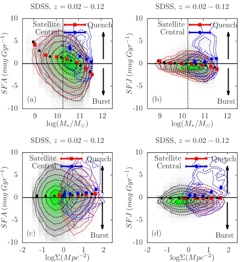
Figure 3 (a) shows the SFA as a function of stellar mass for our SDSS sample (black triangles). A positive (negative) value indicates recent quenching (bursting) in the past 300 Myr. We clearly see a trend with stellar mass, in the sense that on average, less massive galaxies tend to be quenching and more massive systems burst-ing, consistent with Martin et al. (2017). The transition between quenching and bursting occurs at log(M∗/M⊙) ∼ 10.5-11. Figure 3 (b) shows the SFJ versus stellar mass for our local universe sample. A positive (negative) value indicates past quenching (bursting) at 600-300 Myr prior to observations. We still see a very weak correla-tion between SFJ and M∗ particularly at log(M∗/M⊙)

& 11 but clearly, much of the quenching/bursting has happened recently as seen in Figure 3 (a). This indicates that the physics of mass quenching/bursting acts in a relatively short timescale (.300 Myr).

Figures 3 (a) and (b) also show the SFA and SFJ ver-sus M∗ for central and satellite galaxies. To minimize

the projection and group selection effects and contami-nation by interlopers, we only consider satellites and cen-trals that are in groups with > 10 members. Satellites follow the general trends between SFA and SFJ versus M∗. Centrals follow the same slope between SFA and

M∗. However, centrals tend to avoid the bursting

region and at a given M∗, centrals are quenchier

than satellites.

Figures 3 (c) and (d) show the role of the local en-vironment (Σ) on the SFA and SFJ. When averaged over all stellar masses, we find no clear trend (at best a weak correlation) between SFA (or SFJ) and Σ. Ex-cept for an increasing SFJ for centrals in dense regions, satellites and centrals do not show any significant envi-ronmental dependence in their very recent (<300 Myr) and less recent (past 300-600 Myr) quenching/bursting as denoted by SFA and SFJ quantities (when averaged over all stellar masses). This indicates that local envi-ronment likely acts effectively on a much longer timescale when averaged over allM∗. There are other possibilities

too. For example, the local environment might not af-fect the quantities that are linked to quenching/bursting of galaxies. It might also be due to the mass quench-ing/bursting being more effective than the environmen-tal quenching/bursting when averaged over the general population of galaxies.

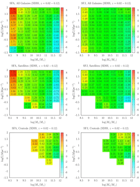
We further investigate the quenching/bursting of galaxies by dividing our sample into stellar mass, sSFR, and density bins. Figure 4 shows the median SFA and SFJ (shown by color) on the logΣ vs. log(M∗/M⊙) plane

for all galaxies, satellites, and centrals. The top number in each cell is the median value and the bottom one is its uncertainty. The mass dependence of SFA is clearly seen on the logΣ versus log(M∗/M⊙) diagram, in a sense

that in any given environment, more massive systems are burstier than less massive galaxies. However, the local environmental dependence of SFA is also evident. In each mass bin, on average, denser environments host higher quenchiness than the less-dense field. The largest burstiness occurs in massive field galaxies (log(M∗/M⊙)

be--10 -5 0 5 10

9 10 11 12

S

F

A

(

m

ag

G

y

r

−

1

)

log

(

M

∗

/M

⊙

)

z

= 0

.

02

−

0

.

12

-10 -5 0 5 10

9 10 11 12

S

F

J

(

m

ag

G

y

r

−

1

)

log

(

M

∗

/M

⊙

)

z

= 0

.

02

−

0

.

12

-10 -5 0 5 10

-2 -1 0 1 2

S

F

A

(

m

ag

G

y

r

−

1

)

log

Σ(

M pc

−

2

₎

z

= 0

.

02

−

0

.

12

-10 -5 0 5 10

-2 -1 0 1 2

S

F

J

(

m

ag

G

y

r

−

1

)

log

Σ(

M pc

−

2

₎

z

= 0

.

02

−

0

.

12

Central

Quenh

Burst (a)

Satellite

Central

Quenh

Burst (b)

Satellite

Central

Quenh

Burst ()

Satellite

Central

Quenh

Burst (d)

-1.5 -1 -0.5 0 0.5 1 1.5 2

8.5 9 9.5 10 10.5 11 11.5 12

lo g Σ ( M pc − 2)

log(M

∗/M⊙)

SFA,AllGalaxies(SDSS,z= 0.02−0.12)

-1.5 -1 -0.5 0 0.5 1 1.5 2

8.5 9 9.5 10 10.5 11 11.5 12

lo g Σ ( M pc − 2 )

log(M

∗/M⊙)

SFJ,AllGalaxies(SDSS,z= 0.02−0.12)

-1.5 -1 -0.5 0 0.5 1 1.5 2

8.5 9 9.5 10 10.5 11 11.5 12

lo g Σ ( M pc − 2)

log(M

∗/M⊙)

SFA,Satellites (SDSS,z= 0.02−0.12)

-1.5 -1 -0.5 0 0.5 1 1.5 2

8.5 9 9.5 10 10.5 11 11.5 12

lo g Σ ( M pc − 2 )

log(M

∗/M⊙)

SFJ,Satellites (SDSS,z= 0.02−0.12)

-1.5 -1 -0.5 0 0.5 1 1.5 2

8.5 9 9.5 10 10.5 11 11.5 12

lo g Σ ( M pc − 2)

log(M

∗/M⊙)

SFA,Centrals(SDSS,z= 0.02−0.12)

-1.5 -1 -0.5 0 0.5 1 1.5 2

8.5 9 9.5 10 10.5 11 11.5 12

lo g Σ ( M pc − 2 )

log(M

∗/M⊙)

SFJ,Centrals(SDSS,z= 0.02−0.12) -2.18 1.22 3.75 1.01 5.02 0.38 3.87 0.37 4.50 0.57 5.81 1.05 7.70 1.75 -0.06 0.89 1.25 0.22 0.97 0.12 1.55 0.13 1.91 0.15 1.46 0.29 2.29 0.45 0.83 0.24 0.98 0.09 0.92 0.06 0.92 0.07 1.14 0.09 1.29 0.14 1.72 0.22 0.83 0.12 1.02 0.04 1.08 0.03 1.15 0.03 1.16 0.04 1.28 0.07 1.01 0.12 0.26 0.09 0.26 0.03 0.35 0.02 0.40 0.02 0.49 0.03 0.55 0.05 0.54 0.09 -1.21 0.15 -0.96 0.04 -0.81 0.02 -0.76 0.03 -0.46 0.04 -0.20 0.06 0.65 0.11 -2.63 0.61 -2.65 0.13 -2.41 0.08 -2.15 0.08 -1.99 0.12 -1.20 0.21 0.35 0.45 -8 -6 -4 -2 0 2 4 6 8 2.52 0.46 1.67 0.28 1.38 0.14 1.13 0.15 1.42 0.23 2.37 0.48 2.25 0.40 0.62 0.15 0.52 0.05 0.35 0.03 0.33 0.03 0.36 0.04 0.33 0.08 0.43 0.11 0.25 0.06 0.14 0.02 0.11 0.01 0.13 0.02 0.10 0.02 0.08 0.04 0.11 0.09 -0.05 0.03 -0.04 0.01 -0.01 0.01 -0.01 0.01 0.00 0.01 -0.01 0.02 -0.16 0.06 -0.19 0.03 -0.20 0.01 -0.20 0.01 -0.19 0.01 -0.18 0.01 -0.14 0.02 -0.25 0.05 -0.59 0.06 -0.56 0.02 -0.50 0.01 -0.51 0.01 -0.40 0.02 -0.36 0.04 0.46 0.10 -0.98 0.26 -1.26 0.07 -1.10 0.05 -1.11 0.05 -0.97 0.07 -0.20 0.16 0.68 0.41 -8 -6 -4 -2 0 2 4 6 8 3.90 0.43 4.75 0.63 5.81 1.05 7.70 1.75 1.76 0.42 1.80 0.17 1.46 0.29 2.29 0.45 -0.13 1.43 3.00 1.59 1.18 0.22 1.09 0.11 1.28 0.14 1.72 0.22 2.35 4.68 1.29 0.64 0.97 0.12 1.11 0.05 1.27 0.07 1.01 0.12 0.54 0.48 0.74 0.28 0.20 0.08 0.44 0.04 0.53 0.05 0.51 0.09 -1.54 0.39 -1.53 0.58 -1.04 0.13 -0.69 0.05 -0.38 0.06 0.46 0.11 -3.75 0.21 -3.73 0.75 -2.83 0.22 -2.23 0.24 -2.23 0.74 -8 -6 -4 -2 0 2 4 6 8 0.15 0.23 1.49 0.24 2.37 0.48 2.25 0.40 0.31 0.09 0.27 0.05 0.33 0.08 0.43 0.11 -0.16 0.35 0.81 0.59 0.10 0.06 0.07 0.03 0.08 0.04 0.11 0.09 1.21 0.80 0.22 0.15 -0.07 0.03 -0.00 0.02 -0.01 0.02 -0.16 0.06 -0.21 0.20 0.00 0.09 -0.27 0.03 -0.19 0.02 -0.14 0.02 -0.27 0.05 -1.08 0.55 -1.25 0.27 -0.64 0.07 -0.46 0.03 -0.44 0.04 0.20 0.10 -2.62 0.55 -1.12 0.36 -1.39 0.11 -1.11 0.14 -1.49 0.48 -8 -6 -4 -2 0 2 4 6 8 2.97 0.69 4.16 2.22 2.07 0.36 1.91 0.25 2.03 0.42 3.46 1.44 2.32 0.37 0.99 0.22 1.02 0.10 1.12 0.16 2.08 0.28 -1.32 0.42 -0.61 0.21 0.71 0.22 0.78 0.32 -8 -6 -4 -2 0 2 4 6 8 0.67 0.13 0.78 0.68 0.35 0.24 0.30 0.20 0.37 0.47 0.56 0.47 1.00 0.48 0.39 0.20 0.61 0.10 1.12 0.22 2.29 0.34 -1.30 0.27 -0.16 0.17 1.46 0.27 1.73 0.58 -8 -6 -4 -2 0 2 4 6 8

-6 -5 -4 -3 -2 -1 0

8.5 9 9.5 10 10.5 11 11.5 12

lo g ( sS F R )( G y r − 1 ) log(M

∗/M⊙)

SFA,AllGalaxies(SDSS,z= 0.02−0.12)

-6 -5 -4 -3 -2 -1 0

8.5 9 9.5 10 10.5 11 11.5 12

lo g ( sS F R )( G y r − 1) log(M

∗/M⊙)

SFJ,AllGalaxies(SDSS,z= 0.02−0.12)

-6 -5 -4 -3 -2 -1 0

8.5 9 9.5 10 10.5 11 11.5 12

lo g ( sS F R )( G y r − 1 ) log(M

∗/M⊙)

SFA,Satellites(SDSS,z= 0.02−0.12)

-6 -5 -4 -3 -2 -1 0

8.5 9 9.5 10 10.5 11 11.5 12

lo g ( sS F R )( G y r − 1) log(M

∗/M⊙)

SFJ,Satellites(SDSS,z= 0.02−0.12)

-6 -5 -4 -3 -2 -1 0

8.5 9 9.5 10 10.5 11 11.5 12

lo g ( sS F R )( G y r − 1 ) log(M

∗/M⊙)

SFA,Centrals(SDSS,z= 0.02−0.12)

-6 -5 -4 -3 -2 -1 0

8.5 9 9.5 10 10.5 11 11.5 12

lo g ( sS F R )( G y r − 1 ) log(M

∗/M⊙)

SFJ,Centrals(SDSS,z= 0.02−0.12) 7.98 0.92 6.86 0.55 5.42 0.23 5.33 0.32 6.75 1.17 3.62 0.75 4.04 0.38 4.17 0.38 2.84 0.25 2.73 0.07 1.41 0.10 3.25 0.53 2.54 0.17 3.55 0.16 4.42 0.17 3.03 0.11 1.72 0.04 0.19 0.06 2.37 0.17 1.60 0.05 1.75 0.07 3.16 0.08 2.59 0.05 1.38 0.02 -0.09 0.04 4.71 0.13 1.42 0.04 0.87 0.03 0.86 0.04 0.94 0.03 0.48 0.01 -1.21 0.03 5.13 0.12 1.65 0.06 0.68 0.03 -0.76 0.03 -0.96 0.02 -0.77 0.02 -3.61 0.08 4.40 0.63 1.52 0.48 0.29 0.10 -1.82 0.08 -2.27 0.05 -2.78 0.14 -7.78 0.46 -8 -6 -4 -2 0 2 4 6 8 3.67 0.52 2.50 0.39 0.80 0.09 0.59 0.07 2.06 0.53 0.12 0.46 0.80 0.23 1.34 0.21 0.65 0.10 0.10 0.02 0.21 0.02 -0.60 0.23 -0.10 0.11 0.71 0.09 1.38 0.10 0.77 0.05 -0.06 0.01 0.02 0.01 -0.49 0.11 -0.40 0.04 0.24 0.05 0.94 0.04 0.69 0.02 -0.07 0.01 -0.15 0.01 4.85 0.10 -0.36 0.03 0.08 0.03 0.18 0.03 0.10 0.02 -0.23 0.01 -0.32 0.01 5.86 0.08 -0.07 0.07 0.11 0.04 -0.46 0.02 -0.62 0.02 -0.55 0.01 -0.50 0.01 6.57 0.35 0.87 0.72 0.07 0.13 -1.11 0.06 -1.16 0.04 -1.30 0.06 -0.74 0.07 -8 -6 -4 -2 0 2 4 6 8 7.84 0.47 6.62 0.73 5.38 0.45 8.27 1.40 6.85 1.65 3.62 0.65 3.06 0.57 4.17 0.63 2.19 0.38 2.56 0.14 1.29 0.24 3.08 0.56 2.11 0.22 3.17 0.25 3.39 0.35 2.80 0.18 1.33 0.09 -0.03 0.18 2.56 0.34 1.45 0.07 1.51 0.11 2.52 0.13 2.06 0.10 1.18 0.05 -0.39 0.11 4.69 0.28 1.31 0.06 0.72 0.05 0.52 0.08 0.75 0.07 0.42 0.04 -1.60 0.11 4.38 0.26 1.52 0.13 0.53 0.06 -0.61 0.07 -0.95 0.07 -1.02 0.08 -3.87 0.25 -0.70 5.23 -0.96 2.54 0.18 0.28 -2.11 0.23 -2.47 0.16 -3.40 0.44 -7.76 1.84 -8 -6 -4 -2 0 2 4 6 8 3.54 0.49 1.70 0.54 0.68 0.12 1.20 0.09 2.53 0.75 0.12 0.46 0.39 0.35 1.52 0.36 0.54 0.12 0.14 0.04 0.18 0.06 -0.73 0.22 -0.21 0.16 0.51 0.16 1.02 0.18 0.76 0.09 -0.10 0.02 -0.02 0.04 -0.53 0.18 -0.49 0.06 0.08 0.08 0.68 0.08 0.50 0.05 -0.10 0.01 -0.12 0.02 4.78 0.25 -0.43 0.05 0.06 0.06 0.02 0.05 0.02 0.04 -0.25 0.01 -0.31 0.02 5.85 0.15 -0.02 0.20 -0.04 0.09 -0.37 0.06 -0.58 0.04 -0.64 0.03 -0.50 0.05 0.14 5.72 -1.44 1.92 0.10 0.33 -1.33 0.18 -1.26 0.11 -1.50 0.19 -1.00 0.19 -8 -6 -4 -2 0 2 4 6 8 4.01 0.03 6.16 0.47 2.00 0.19 1.40 0.21 2.93 1.14 1.06 0.64 1.47 0.37 5.28 0.22 2.06 0.18 1.29 0.08 0.16 0.13 -0.32 0.27 0.25 0.15 -0.63 0.23 4.94 0.72 5.22 0.93 0.84 0.13 -0.60 0.17 -2.06 0.25 -2.13 0.54 -3.62 4.23 -8 -6 -4 -2 0 2 4 6 8 0.49 0.30 4.59 0.35 0.29 0.37 0.69 0.29 1.37 0.23 -0.44 0.18 0.22 0.04 5.69 0.15 0.19 0.25 1.48 0.10 0.87 0.12 -0.02 0.16 -0.15 0.09 -0.29 0.02 6.66 0.45 6.81 0.54 1.43 0.11 0.47 0.16 -0.83 0.20 -0.89 0.16 -0.47 0.37 -8 -6 -4 -2 0 2 4 6 8

-6 -5 -4 -3 -2 -1 0

-1.5 -1 -0.5 0 0.5 1 1.5 2

lo g ( sS F R )( G y r − 1 )

logΣ(M pc−

2 )

SFA,AllGalaxies(SDSS,z= 0.02−0.12)

-6 -5 -4 -3 -2 -1 0

-1.5 -1 -0.5 0 0.5 1 1.5 2

lo g ( sS F R )( G y r − 1)

logΣ(M pc−

2 )

SFJ,AllGalaxies(SDSS,z= 0.02−0.12)

-6 -5 -4 -3 -2 -1 0

-1.5 -1 -0.5 0 0.5 1 1.5 2

lo g ( sS F R )( G y r − 1 )

logΣ(M pc

−2

)

SFA,Satellites(SDSS,z= 0.02−0.12)

-6 -5 -4 -3 -2 -1 0

-1.5 -1 -0.5 0 0.5 1 1.5 2

lo g ( sS F R )( G y r − 1)

logΣ(M pc

−2

)

SFJ,Satellites(SDSS,z= 0.02−0.12)

-6 -5 -4 -3 -2 -1 0

-1.5 -1 -0.5 0 0.5 1 1.5 2

lo g ( sS F R )( G y r − 1 )

logΣ(M pc−

2 )

SFA,Centrals(SDSS,z= 0.02−0.12)

-6 -5 -4 -3 -2 -1 0

-1.5 -1 -0.5 0 0.5 1 1.5 2

lo g ( sS F R )( G y r − 1 )

logΣ(M pc−

2 )

SFJ,Centrals(SDSS,z= 0.02−0.12) 1.11 0.94 1.62 0.46 0.97 0.25 0.51 0.32 0.47 0.23 0.67 0.07 -0.69 0.15 3.68 0.46 1.47 0.10 1.10 0.07 0.51 0.09 0.20 0.06 0.64 0.02 -0.72 0.05 4.24 0.18 1.59 0.06 0.95 0.04 0.11 0.05 0.11 0.03 0.64 0.02 -0.80 0.03 4.44 0.19 1.52 0.05 0.94 0.04 0.12 0.05 0.18 0.04 0.63 0.02 -0.74 0.04 4.80 0.16 1.52 0.06 0.86 0.05 0.24 0.06 0.25 0.05 0.67 0.03 -0.84 0.07 4.14 0.27 1.53 0.07 0.90 0.05 0.27 0.08 0.45 0.09 0.69 0.06 -1.23 0.15 4.69 0.34 1.50 0.11 0.92 0.07 0.19 0.14 0.44 0.21 0.83 0.15 -1.91 0.38 -8 -6 -4 -2 0 2 4 6 8 -0.78 0.06 -0.18 0.26 -0.37 0.19 0.12 0.14 -0.07 0.12 -0.17 0.02 -0.15 0.02 4.35 0.77 -0.34 0.07 0.08 0.06 -0.04 0.05 -0.12 0.03 -0.20 0.01 -0.21 0.01 4.92 0.20 -0.24 0.04 0.12 0.04 -0.10 0.03 -0.14 0.02 -0.19 0.01 -0.22 0.01 5.02 0.16 -0.28 0.04 0.16 0.04 -0.04 0.03 -0.14 0.02 -0.20 0.01 -0.21 0.01 5.14 0.13 -0.29 0.05 0.06 0.05 0.05 0.04 -0.12 0.03 -0.19 0.01 -0.20 0.01 4.45 0.33 -0.37 0.05 0.24 0.06 0.02 0.06 -0.03 0.04 -0.20 0.02 -0.11 0.03 5.03 0.31 -0.40 0.10 0.37 0.10 0.30 0.09 0.04 0.10 -0.23 0.04 -0.18 0.08 -8 -6 -4 -2 0 2 4 6 8 -0.29 1.31 -1.39 0.94 0.28 1.59 1.26 0.45 -1.30 0.17 0.11 1.72 3.01 3.48 0.38 1.11 0.81 0.68 0.84 0.29 -1.06 0.73 2.66 0.90 1.28 0.17 0.95 0.18 0.64 0.20 0.61 0.16 0.59 0.08 -0.64 0.18 3.84 0.29 1.46 0.07 0.86 0.06 0.36 0.08 0.43 0.07 0.67 0.04 -0.80 0.09 3.22 0.36 1.47 0.07 0.86 0.06 0.29 0.09 0.51 0.09 0.68 0.06 -1.23 0.15 4.54 0.40 1.47 0.11 0.87 0.08 0.19 0.14 0.44 0.21 0.83 0.15 -1.91 0.38 -8 -6 -4 -2 0 2 4 6 8 -1.54 0.39 -1.38 0.31 0.25 1.26 -0.27 0.18 0.08 0.08 -1.32 0.66 1.03 1.86 0.10 0.54 0.11 0.34 -0.19 0.09 -0.15 0.14 2.09 1.69 -0.20 0.13 0.04 0.16 -0.10 0.12 0.03 0.08 -0.23 0.02 -0.24 0.03 4.79 0.42 -0.31 0.06 0.01 0.06 0.03 0.05 -0.04 0.03 -0.18 0.01 -0.16 0.02 0.45 0.44 -0.38 0.06 0.13 0.07 -0.08 0.06 -0.01 0.04 -0.20 0.02 -0.11 0.03 4.50 0.49 -0.52 0.09 0.23 0.10 0.25 0.10 0.04 0.10 -0.23 0.04 -0.18 0.08 -8 -6 -4 -2 0 2 4 6 8 5.26 0.70 2.07 0.30 1.42 0.28 -0.56 0.49 0.23 0.45 0.22 0.21 5.28 0.35 2.01 0.21 1.11 0.10 0.11 0.16 -0.48 0.26 0.53 0.24 -0.94 0.26 5.25 0.30 2.44 0.30 1.05 0.13 -0.17 0.18 -1.92 0.39 -0.06 0.38 5.56 0.76 3.68 0.84 1.39 0.21 -0.25 0.36 -2.11 2.15 -8 -6 -4 -2 0 2 4 6 8 5.05 0.64 0.19 0.42 1.57 0.27 0.32 0.44 -0.07 0.30 -0.09 0.13 5.41 0.17 0.06 0.27 1.17 0.11 0.49 0.12 -0.43 0.15 -0.09 0.10 -0.31 0.07 5.52 0.22 0.28 0.34 1.45 0.11 1.05 0.20 -0.83 0.28 -0.12 0.18 6.15 0.46 3.64 1.25 1.85 0.20 1.02 0.27 -1.01 0.30 -8 -6 -4 -2 0 2 4 6 8

-10 -5 0 5 10

10 11 12

S

F

A

(

m

ag

G

y

r

−

1

)

log

(

M

∗

/M

⊙

)

LEGA-C,

z

≈

0

.

6

−

1

.

0

-10 -5 0 5 10

10 11 12

S

F

J

(

m

ag

G

y

r

−

1

)

log

(

M

∗

/M

⊙

)

LEGA-C,

z

≈

0

.

6

−

1

.

0

-10 -5 0 5 10

-1 0 1

S

F

A

(

m

ag

G

y

r

−

1

)

log

Σ(

M pc

−

2

₎

z

≈

0

.

6

−

1

.

0

-10 -5 0 5 10

-1 0 1

S

F

J

(

m

ag

G

y

r

−

1

)

log

Σ(

M pc

−

2

₎

z

≈

0

.

6

−

1

.

0

Central

Quenh

Burst (a)

Satellite

Central

Quenh

Burst (b)

Satellite

Central

Quenh

Burst ()

Satellite

Central

Quenh

Burst (d)

-1.5 -1 -0.5 0 0.5 1 1.5 2

8.5 9 9.5 10 10.5 11 11.5 12

lo g Σ ( M pc − 2) log(M

∗/M⊙)

SFA,AllGalaxies(LEGA-C,z≈0.6−1.0)

-1.5 -1 -0.5 0 0.5 1 1.5 2

8.5 9 9.5 10 10.5 11 11.5 12

lo g Σ ( M pc − 2 ) log(M

∗/M⊙)

SFJ,AllGalaxies(LEGA-C,z≈0.6−1.0)

-1.5 -1 -0.5 0 0.5 1 1.5 2

8.5 9 9.5 10 10.5 11 11.5 12

lo g Σ ( M pc − 2) log(M

∗/M⊙)

SFA,Satellites(LEGA-C,z≈0.6−1.0)

-1.5 -1 -0.5 0 0.5 1 1.5 2

8.5 9 9.5 10 10.5 11 11.5 12

lo g Σ ( M pc − 2 ) log(M

∗/M⊙)

SFJ,Satellites(LEGA-C,z≈0.6−1.0)

-1.5 -1 -0.5 0 0.5 1 1.5 2

8.5 9 9.5 10 10.5 11 11.5 12

lo g Σ ( M pc − 2) log(M

∗/M⊙)

SFA,Centrals(LEGA-C,z≈0.6−1.0)

-1.5 -1 -0.5 0 0.5 1 1.5 2

8.5 9 9.5 10 10.5 11 11.5 12

lo g Σ ( M pc − 2 ) log(M

∗/M⊙)

SFJ,Centrals(LEGA-C,z≈0.6−1.0) 1.99 1.37 1.77 0.04 0.76 5.88 3.76 0.78 2.65 0.92 2.53 2.54 2.14 0.12 1.72 0.47 1.09 0.23 2.54 0.35 1.08 0.33 -1.59 1.40 0.14 0.48 0.72 0.23 0.49 0.22 1.00 0.58 -0.68 0.27 -5.77 2.64 -0.75 0.80 -1.39 0.94 -8 -6 -4 -2 0 2 4 6 8 0.54 0.56 0.56 0.72 0.49 4.16 0.27 0.36 0.72 0.37 1.06 1.53 0.81 0.60 0.06 0.20 0.05 0.09 1.08 0.27 0.02 0.14 -0.60 0.03 -0.48 0.16 -0.15 0.10 -0.26 0.07 0.21 0.40 1.76 2.36 -1.00 1.63 -0.48 0.90 2.29 0.94 -8 -6 -4 -2 0 2 4 6 8 4.52 1.11 2.53 3.17 3.81 2.88 0.56 0.36 2.20 0.42 1.08 0.33 -1.59 2.00 0.23 0.48 -0.02 0.26 1.00 0.35 -0.87 2.12 -4.25 2.92 -8 -6 -4 -2 0 2 4 6 8 1.69 0.74 1.06 1.29 2.68 2.76 -0.14 0.11 0.27 0.25 0.02 0.14 -0.76 0.41 -0.10 0.16 -0.48 0.08 -0.06 0.23 -0.06 0.72 0.18 3.24 -8 -6 -4 -2 0 2 4 6 8 5.28 2.77 2.20 0.06 2.36 2.14 2.45 0.42 3.23 0.74 0.34 0.94 0.45 0.33 1.40 0.25 2.93 0.97 -5.23 3.17 -0.62 0.14 -0.13 1.24 -8 -6 -4 -2 0 2 4 6 8 2.28 1.63 1.33 0.41 0.21 0.90 0.87 0.32 1.45 0.47 0.08 0.44 -0.09 0.20 0.04 0.15 1.49 0.26 -1.45 2.21 -0.91 1.82 2.58 1.34 -8 -6 -4 -2 0 2 4 6 8

-6 -5 -4 -3 -2 -1 0

8.5 9 9.5 10 10.5 11 11.5 12

lo g ( sS F R )( G y r − 1 ) log(M

∗/M⊙)

SFA,AllGalaxies(LEGA-C,z≈0.6−1.0)

-6 -5 -4 -3 -2 -1 0

8.5 9 9.5 10 10.5 11 11.5 12

lo g ( sS F R )( G y r − 1) log(M

∗/M⊙)

SFJ,AllGalaxies(LEGA-C,z≈0.6−1.0)

-6 -5 -4 -3 -2 -1 0

8.5 9 9.5 10 10.5 11 11.5 12

lo g ( sS F R )( G y r − 1 ) log(M

∗/M⊙)

SFA,Satellites (LEGA-C,z≈0.6−1.0)

-6 -5 -4 -3 -2 -1 0

8.5 9 9.5 10 10.5 11 11.5 12

lo g ( sS F R )( G y r − 1) log(M

∗/M⊙)

SFJ,Satellites (LEGA-C,z≈0.6−1.0)

-6 -5 -4 -3 -2 -1 0

8.5 9 9.5 10 10.5 11 11.5 12

lo g ( sS F R )( G y r − 1 ) log(M

∗/M⊙)

SFA,Centrals(LEGA-C,z≈0.6−1.0)

-6 -5 -4 -3 -2 -1 0

8.5 9 9.5 10 10.5 11 11.5 12

lo g ( sS F R )( G y r − 1 ) log(M

∗/M⊙)

SFJ,Centrals(LEGA-C,z≈0.6−1.0) 1.99 1.37 1.56 2.27 5.76 0.84 4.67 1.02 0.09 0.54 0.80 0.99 2.42 0.57 2.84 0.23 1.63 0.31 0.64 0.21 0.23 0.67 1.06 0.34 1.61 0.26 0.98 0.17 -0.88 0.30 -6.17 0.37 -0.94 0.21 -0.65 0.86 -0.45 0.74 -2.29 1.96 -8 -6 -4 -2 0 2 4 6 8 0.54 0.56 0.24 0.34 3.42 0.58 1.69 0.54 -0.16 0.07 2.10 0.63 1.86 0.30 1.32 0.22 0.03 0.09 -0.15 0.04 0.16 0.75 0.49 0.35 0.28 0.30 -0.07 0.09 -0.52 0.04 -2.97 0.69 3.86 0.58 0.91 2.47 -0.85 0.16 -0.69 0.21 -8 -6 -4 -2 0 2 4 6 8 4.52 1.94 4.98 1.00 2.20 1.40 0.80 1.18 2.15 1.21 2.58 0.28 0.44 0.43 0.47 0.22 0.78 0.23 0.21 0.58 1.42 0.65 0.80 0.34 -1.50 0.43 -2.71 4.53 -8 -6 -4 -2 0 2 4 6 8 3.73 0.76 1.69 0.32 0.13 0.20 2.10 1.18 1.87 0.89 0.93 0.28 -0.06 0.20 -0.23 0.06 0.05 0.22 0.01 0.39 0.28 0.48 -0.21 0.13 -0.57 0.07 -1.48 1.49 -8 -6 -4 -2 0 2 4 6 8 2.51 0.89 2.74 0.40 2.30 0.56 0.26 0.95 1.70 0.91 1.86 0.49 1.61 0.33 1.04 0.12 -0.06 0.31 -6.17 0.15 -0.97 0.88 -8 -6 -4 -2 0 2 4 6 8 1.45 0.33 1.34 0.18 0.41 0.29 -0.31 0.15 1.46 0.77 0.62 0.21 0.30 0.25 0.06 0.23 -0.54 0.09 -3.91 0.92 2.58 1.33 -0.85 0.07 -8 -6 -4 -2 0 2 4 6 8

-6 -5 -4 -3 -2 -1 0

-1.5 -1 -0.5 0 0.5 1 1.5 2

lo g ( sS F R )( G y r − 1 )

logΣ(M pc

−2

)

SFA,AllGalaxies(LEGA-C,z≈0.6−1.0)

-6 -5 -4 -3 -2 -1 0

-1.5 -1 -0.5 0 0.5 1 1.5 2

lo g ( sS F R )( G y r − 1)

logΣ(M pc

−2

)

SFJ,AllGalaxies(LEGA-C,z≈0.6−1.0)

-6 -5 -4 -3 -2 -1 0

-1.5 -1 -0.5 0 0.5 1 1.5 2

lo g ( sS F R )( G y r − 1 )

logΣ(M pc

−2

)

SFA,Satellites (LEGA-C,z≈0.6−1.0)

-6 -5 -4 -3 -2 -1 0

-1.5 -1 -0.5 0 0.5 1 1.5 2

lo g ( sS F R )( G y r − 1)

logΣ(M pc

−2

)

SFJ,Satellites (LEGA-C,z≈0.6−1.0)

-6 -5 -4 -3 -2 -1 0

-1.5 -1 -0.5 0 0.5 1 1.5 2

lo g ( sS F R )( G y r − 1 )

logΣ(M pc

−2

)

SFA,Centrals(LEGA-C,z≈0.6−1.0)

-6 -5 -4 -3 -2 -1 0

-1.5 -1 -0.5 0 0.5 1 1.5 2

lo g ( sS F R )( G y r − 1 )

logΣ(M pc

−2

)

SFJ,Centrals(LEGA-C,z≈0.6−1.0) 4.46 1.74 2.14 0.16 -1.70 0.51 0.85 0.89 1.72 0.44 2.24 0.47 -0.29 0.48 -0.24 1.30 2.08 0.48 2.56 0.27 1.07 0.25 0.12 0.23 1.60 0.50 1.86 0.61 2.81 0.39 0.77 0.31 0.27 0.28 0.57 0.67 0.63 0.83 2.38 0.88 1.27 0.17 -1.50 1.87 -1.29 1.26 -8 -6 -4 -2 0 2 4 6 8 2.90 2.32 0.68 0.11 -0.58 0.03 0.15 1.10 0.21 0.42 0.55 0.19 -0.49 0.12 0.61 1.32 1.07 0.33 1.10 0.26 0.00 0.09 -0.27 0.04 -0.40 0.33 1.88 0.70 1.27 0.26 -0.10 0.11 -0.26 0.05 0.16 1.24 1.40 0.91 1.93 0.52 0.01 0.28 -0.57 0.21 0.51 1.41 -8 -6 -4 -2 0 2 4 6 8 1.24 0.19 -1.59 0.89 1.39 1.34 1.98 0.32 1.64 0.75 0.09 0.38 1.29 0.54 0.08 0.52 3.12 0.19 0.19 0.26 0.17 0.26 0.58 0.27 1.82 2.03 1.27 0.17 -1.50 1.87 -8 -6 -4 -2 0 2 4 6 8 -0.05 0.10 -0.76 0.44 0.93 1.42 0.69 0.31 0.24 0.25 -0.28 0.06 -0.27 0.37 1.86 1.03 1.28 0.41 -0.16 0.13 -0.27 0.07 0.16 1.47 1.98 1.10 0.01 0.28 -0.57 0.21 -8 -6 -4 -2 0 2 4 6 8 1.81 0.84 -1.04 1.52 -0.94 3.54 1.82 0.54 2.16 0.35 1.09 0.38 -0.73 0.43 1.70 0.74 2.19 0.68 1.62 0.31 1.16 0.59 1.02 0.29 1.06 1.57 -8 -6 -4 -2 0 2 4 6 8 1.29 0.49 -0.51 0.31 1.90 1.11 0.75 0.39 0.82 0.38 0.10 0.22 -0.60 0.15 -0.40 1.74 2.09 0.75 1.06 0.24 0.04 0.32 -0.20 0.04 1.49 0.85 -8 -6 -4 -2 0 2 4 6 8

-5 0 5

9 10 11 12

S

F

A

(

m

ag

G

y

r

−

1)

log(M∗/M⊙)

-5 0 5

9 10 11 12

S

F

J

(

m

ag

G

y

r

−

1)

log(M∗/M⊙)

-5 0 5

-2 -1 0 1 2

S

F

A

(

m

ag

G

y

r

−

1)

logΣ(M pc

−2₎

-5 0 5

-2 -1 0 1 2

S

F

J

(

m

ag

G

y

r

−

1 )

logΣ(M pc

−2₎

-5 0 5

-6 -4 -2 0

S

F

A

(

m

ag

G

y

r

−

1)

log(sSF R)(Gyr

−1₎ -5

0 5

-6 -4 -2 0

S

F

J

(

m

ag

G

y

r

−

1)

log(sSF R)(Gyr

−1₎ loal

high-z

Quenh

Burst (a)

loal high-z

Quenh

Burst (b)

loal high-z

Quenh

Burst ()

loal high-z

Quenh

Burst (d)

loal high-z

Quenh

Burst (e)

loal high-z

Quenh

Burst (f)

Fig. 11.—(a) Median SFA vs. M∗(b) SFJ vs. M∗(c) SFA vs. logΣ (d) SFJ vs. logΣ (e) SFA vs. sSFR and (f) SFJ vs. sSFR for our local universe and high-z samples. On average, at fixedM∗, sSFR, and (to a lesser degree) Σ, the higher redshift galaxies are quenchier. Black vertical line shows the stellar mass completeness limit.

longs to low-mass systems in very dense environments (log(M∗/M⊙).9.0 and logΣ&0.5).

In addition, at fixed Σ, the SFA change with stellar mass is stronger than the SFA change with environment while fixing M∗. In other words, although the SFA

de-pends on both stellar mass and environment, the stellar mass dependence is stronger. Also note that the envi-ronmental dependence of SFA is less significant in the medium range of stellar masses (log(M∗/M⊙)≈9.5-11)

and that is why on average, we do not find a significant environmental dependence of SFA in Figure 3.

Median SFA of satellites follows the general distribu-tion of galaxies and it depends on both stellar mass and environment. However, SFA of centrals only shows a mass dependence and within the uncertainties, it is al-most independent of the local environment (or at best has a weak dependence). This suggests that the environ-mental dependence of SFA is mostly due to satellites.

Note that in each stellar mass and environment bin, centrals are quenchier than satellites and that centrals are mainly quenching. Compared to the SFA, the SFJ shows much weaker dependence onM∗and almost no (or

at best a weak) environmental dependence.

The strong sSFR dependence of the trends investigated so far is also evident in Figures 5 and 6. Figure 5 shows the median SFA and SFJ on the diagram of log(sSFR) versus log(M∗/M⊙) for all galaxies, satellites, and

cen-trals at z ∼ 0. The mass dependence of SFA is also seen on the log(sSFR) versus log(M∗/M⊙) diagram, i.e.;

at fixed sSFR and on average, more massive galaxies are burstier than less massive systems. However, the SFA strongly depends on sSFR as well. At fixed stel-lar mass and on average, the median SFA increases with decreasing sSFR, confirming theM∗-sSFR trend seen in

Martin et al. (2017) for “all galaxies”. In fact, the bursti-ness occurs in massive (log(M∗/M⊙) star-forming

galax-ies with high sSFRs (log(sSFR)(Gyr−1_)&-3).

Similar trends are seen for satellites and centrals, that is, on average, the SFA increase with decreasing stellar mass and sSFR for both satellites and centrals. However, in eachM∗and sSFR bin, centrals quench faster than (at

best have similar SFA to) satellites. Compared to SFA, the SFJ shows weaker dependence on M∗ and sSFR (at

best similar values in massive, low-sSFR galaxies). Finally, the SFA and SFJ as a function of sSFR and local density is shown in Figure 6. At fixed environment, the median SFA depends on sSFR and increases with decreasing sSFR. However, at fixed sSFR and within the uncertainties, the median SFA is almost indepen-dent of the local density of galaxies. These results hold for all galaxies, as well as satellites and centrals. The weaker sSFR and Σ dependence of the SFJ compared to SFA is also seen. Combining the results in

Fig-ures 4, 5, and 6 indicates that at z ∼0, much of

the bursting of star-formation happens in mas-sive, high sSFR galaxies, particularly those in the field (and among group galaxies, satellites more than centrals), whereas most of the quenching of star-formation happens in less-massive, low sSFR galaxies, in particular those located in dense en-vironments. For centrals, quenching is significant even in higher mass systems.

4.2. _{Quenching/Bursting of Galaxies at High-z}

We find similar results atz ∼1 for our LEGA-C sam-ple as shown in Figures 7, 8, 9, and 10. To increase the statistics, all satellites and centrals (with number of group members>2) are included9_{. Also note the smaller}

dynamical range of the environment andM∗probed here

compared to that of the SDSS. Even with these limita-tions, some trends between the SFA (and to a smaller degree, the SFJ) and M∗, sSFR, and to a lesser degree

environment are evident (with evidence of deviation be-tween centrals and satellites). For example, as shown in Figure 7, we find a mass dependence and an environ-mental independence (when averaged over all M∗s and

to logΣ∼1) of the SFA and SFJ atz∼1, with centrals being quenchier than satellites on average.

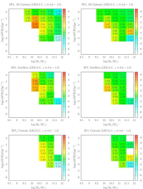
According to Figure 8, the decrease in median SFA with stellar mass (even at fixed environment) is also seen at z ∼ 1. Unfortunately, due to a smaller dynamical

9_{We note that because of this selection, the high-zgroup}

-0.4 0 0.4 0.8 1.2 1.6 2

10 10.5 11 11.5 12

∆

(

m

ag

G

y

r

−

1)

log(M∗/M⊙)

-0.4 0 0.4 0.8 1.2 1.6 2

0 0.5 1 1.5

∆

(

m

ag

G

y

r

−

1)

logΣ(M pc

−2₎

∆SF A

∆SF J

(a)

∆SF A

∆SF J

(b)

Fig. 12.— ∆SF A=|SF A(z ∼ 1) − SF A(z ∼ 0)| and

∆SF J=|SF J(z∼1)−SF J(z∼0)|as a function of stellar mass (a)

and local environment (b). ∆ is defined to investigate the redshift evolution of mass and environmental quenching/bursting. ∆SF A

(and to a lesser degree ∆SF J) values show that the strength of

the recent mass and environmental quenching/bursting is larger at higher redshift.

range of Σ,M∗, and sample size and larger uncertainties

in our high-z sample compared to the local universe, we cannot make a significantly robust statement about the potential SFA relation with environment (at given stellar mass). However, even with these limitations, the over-all sample of galaxies shows signs of increasing SFA (and quenching) in denser environments at fixedM∗. The

stel-lar mass dependence of SFA is also seen for both satel-lites and centrals atz ∼1 but within the uncertainties and in the stellar mass and environment range covered at high-z, no clear relation between SFA and environment is seen when we further break the sample into centrals and satellites. Note that even atz ∼1, centrals seem to be quenchier than satellites in an average sense. Simi-lar to the low-z results, the SFJ shows weakerM∗ and

Σ dependence (if any) than the SFA. More importantly, we find that at given bins of stellar mass and environ-ment, higher z galaxies are on average quenchier than (or within the uncertainties, have at best similar SFAs to) their local-universe counterparts.

Similar to Figure 5, the median SFA decreases with increasing stellar mass and (and to a lesser degree) sSFR for all galaxies, satellites and centrals atz∼1. Moreover, at any given stellar mass and sSFR, higher redshift galax-ies (all, centrals, and satellites) are on average quenchier than (or within uncertainties, have similar SFAs to) their local-universe counterparts. Similar to low-zresults, the SFJ shows weaker (or similar) trends withM∗and sSFR

than the SFA. Given the narrow range of environments and sSFRs, and large uncertainties, no significantly clear trend between SFA and environment or sSFR is seen in Figure 10. However, some environmental bins show signs of an increasing SFA with decreasing sSFR, sim-ilar to the results at low-z. Moreover, at any given Σ and sSFR, higherzgalaxies (all, centrals, and satellites) are on average quenchier than (or within uncertainties, have similar SFAs to) their local-universe counterparts. At fixed sSFR and Σ, the SFJ shows smaller values than (or similar values to) the SFA.

In selecting the group galaxies for the high-z sample, all groups with>2 members are considered. This makes the sample more prone to contamination by interlopers and might lead to unwanted biases when we compare the low- and high-z results. However, in Appendix D, we show that the global trends could still be recovered using groups with>10 members for the high-z sample.

4.3. _{Redshift Evolution of Galaxy Quenching/Bursting}

Comparing the low- and high-zresults indicates

that at fixed M∗, sSFR, and environment, higher

redshift galaxies (all, centrals, and satellites) are on average quenchier than their local-universe

counterparts. This is more clearly seen in Figure 11.

At fixedM∗(averaged over all environments and sSFRs,

top panel), fixed sSFR (averaged over Σ andM∗, bottom

panel), and more slightly at fixed Σ (averaged over sSFR andM∗, middle panel), on average, our high-zsample is

quenchier than the local-universe sample.

To further quantify the redshift evolution of the mass and environmental quenching and potentially com-pare their relative strength, we define the quantity ∆SF A=|SF A(z∼1)−SF A(z∼0)|as the absolute dif-ference between the median SFA atz∼1 (LEGA-C sam-ple) and the median SFA at z ∼0 (SDSS sample). We define a similar quantity for the SFJ (∆SF J=|SF J(z∼

1)−SF J(z∼0)|). This absolute difference is done as a function of both stellar mass and environment and at the common stellar mass and environmental range of values for the high-z and local-universe samples (log(M∗/M⊙) ≈ 10-12 and log(Σ)≈ -0.25-1.5). We model the me-dian SFA(and SFJ) as a function of M∗ and Σ with

linear functions, taking their uncertainties into account. The absolute difference defined in ∆ represents the dif-ference between the linearly-modelled SFA (or SFJ). Figure 12 shows the results. Both stellar mass and environment show stronger strength in recent quench-ing/bursting of galaxies at higher redshift. Moreover, the change in stellar mass quenching/bursting seems to be larger (∆SF A(M∗) ≈ 1.7-0.8 magGyr−1 at 10

.log(M∗/M⊙).12) than the environment (∆SF A(Σ)≈

0.4-0.1 magGyr−1_{at 0.5.log(Σ).1.5) sincez∼1. The}

SFJ shows weaker trends compared to the SFA.

5. _DISCUSSION

Toz∼1, we find that: 1- the SFA (and SFJ to a lesser degree) decreases with increasing stellar mass, increasing sSFR, and decreasing local density. 2- on average, cen-trals quench faster than satellites, and 3- high redshift galaxies are quenchier than their local-universe counter-parts.

To explain the mass dependence of SFA, Martin et al. (2017) proposed a scenario in which lower mass galax-ies accrete into halos and become satellites, having their star-forming gas tidally and/or ram-pressure stripped, while higher mass centrals receive the gas and react with new star formation. However, by explicitly breaking the sample into satellites and centrals, we see the opposite trend, with centrals being quenchier than satellites at fixedM∗, sSFR, and Σ bins in an average sense out toz ∼1.

high sSFR star-forming galaxies. The merger picture might also explain why centrals are quenching faster than satellites, if the dominant wet mergers in centrals had happened much earlier than satellites so that at the present, we are mainly witnessing the quenching phase of the merger. An even older (>600 Myr) star-formation derivative might reveal the past bursting phase of cen-trals. Moreover, whether the wet merger is “major” or “minor” might also explain why centrals are quenching faster than satellites. In other words, the current burst-ing of star-formation in massive satellites might be be-cause of wet major mergers, whereas this recent bursting in massive centrals could be mostly due to wet minor mergers.

Although the wet merger scenario might explain the burstiness of massive galaxies in the field as seen in e.g., Figure 4 (Lin et al. 2010), the merger picture be-comes problematic in denser environments. Mergers are more common in denser environments than the field (es-pecially in group-scales; Perez et al. 2009; Sobral et al. 2011; Tonnesen & Cen 2012) but we see in e.g. Fig-ures 3 and 7 that satellites and the overall galaxy dis-tribution follow similar bursting trends. Moreover, there is evidence that centrals are as old as or even younger than satellites and they are quenched at the same time as or even more recently than satellites of the same mass (Pasquali et al. 2010; Fitzpatrick & Graves 2015; Smethurst et al. 2017). Moreover, mergers in dense en-vironments seem to be mostly dry and the merger-driven history of centrals is mainly due to gas-poor, dry mergers with no significant star-formation (e.g.; McIntosh et al. 2008; Lin et al. 2010; Lidman et al. 2012; Shankar et al. 2015; Davidzon et al. 2016).

By studying SDSS galaxy pairs Ellison et al. (2010) showed that although interactions happen at all environ-ments, interaction-triggered star-formation is seen only in low-to-intermediate density environments. The posi-tion of centrals in the densest regions of groups/clusters is in agreement with this picture and explains why they avoid bursting especially in densest regions as clearly seen in e.g., Figure 4.

There is evidence for the gas fraction being higher in the field galaxies than those in denser environments as previous accretion of galaxies into their current halos made them gas-stripped (Cortese & Hughes 2009; Fabello et al. 2012; Catinella et al. 2013; Boselli & Gavazzi 2014). It is also possible that the cold gas accretion from the surrounding LSS can more easily/efficiently/numerously penetrate isolated and satellite galaxies than centrals that are located in the densest regions of groups/clusters. van de Voort et al. (2017) simulations show that more massive centrals and satellites both have a higher gas accretion rate than less massive ones (also see Dekel et al. 2013). They also find that gas accretion rate is lower or fully suppressed (depending on the halo mass) in the center of halos. They also find a strong environmental dependence of accretion rate primarily for satellites. This might explain the strong quenching of low-mass satellites in denser regions seen in Figure 4. Therefore, a combination of stellar mass and halo-centric and environmental dependence of gas accretion rate, gas fraction, and mergers can potentially explain the observed trends. Further analyses including gas and age dependence of

different galaxy types on SFA, SFJ, local environment, stellar mass, and sSFR can shed light on this.

The recent mass quenching of lower mass galax-ies (log(M∗/M⊙) . 10) might also be partly due to

fast-acting stellar and supernova feedback which is stronger on less massive systems because of their weaker gravitational potential (e.g.; Ceverino & Klypin 2009; Hopkins et al. 2014). However, feedback produces short-timescale burstiness in star formation especially for less massive galaxies (e.g.; Hopkins et al. 2014), which is not clearly seen in the median trends in our results. However, part of this discrepancy might be due to different rates for star-formation burstiness and quenching. That is, when a galaxy bursts, it almost instantly becomes blue but the quenching phase takes longer to act. Therefore, the av-erage in bins of M∗-sSFR would be quenching because

of this asymmetry. Rapid AGN feedback on less mas-sive galaxies can also have some effect in their quenching (Smethurst et al. 2017).

The higher quenching of our high-z sample compared to SDSS, even at fixed M∗, sSFR, and environment

might be due to a faster and more efficient quenching rate at higher redshifts. By studying a large sample of transiting galaxies at z ∼ 1, Gon¸calves et al. (2012) showed that mass flux from the blue cloud to the red sequence (through the green valley) is larger at z ∼

1 compared to the same quantity in the local universe (Martin et al. 2007). The faster quenching rate of tran-siting galaxies atz∼1 has been recently reconfirmed by Nogueira-Cavalcante et al. (2018). In this paper, how-ever, we find that this seems to be true for all galaxies (not just transiting systems) and even satellites and cen-trals. Quenching, regardless of the process, is stronger at z∼1 for all galaxies at all stellar masses, sSFRs, and Σs. In agreement with our results, Tinker & Wetzel (2010) and Quadri et al. (2012) showed that satellite quench-ing must proceed faster at high redshift. Moreover, McGee et al. (2014) argued that given the strong red-shift evolution of the star-formation rate, the quenching timescales should be shorter at higher redshift. Recently, Rowlands et al. (2018) also found a faster quenching at z ∼0.7 than the local universe.

Out toz ∼1, the local environment seems to have a milder effect (if any) on the SFA and SFJ, with stellar mass (and sSFR) being the dominant factor over a large range of M∗, Σ, sSFRs and redshift. The dominance of

“mass quenching” over “environmental quenching” has been found, particularly for more massive galaxies and at higher redshifts (e.g.; Peng et al. 2010; Darvish et al. 2016; Smethurst et al. 2017). Only very dense environ-ments seem to significantly influence the SFA, particu-larly for the least massive satellites. Ram pressure strip-ping and other environmentally-driven processes that are practically effective on less massive galaxies might be causing this, whereas mergers are likely behind the trends for more massive galaxies in the field.

Crossett et al. 2017). In addition, simulations of group and cluster galaxies by Bah´e & McCarthy (2015) show that ram pressure stripping is more affective at z ∼ 1 than z=0, in agreement with a higher SFA we find for our high-zsample compared to that of the local-universe at a fixed local environment. We further note that our results indicate that mass quenching likely happens in short timescales, while the opposite is likely true for en-vironmental quenching (at least when averaged over the whole population). That threshold, established by our methodology (especially given the lack of the SFJ at slightly longer timescales) might set an interesting com-parison basis for future studies. Further studies using a modified SFA measure derived over a long timescale are needed to investigate this.

Using Martin et al. (2017) method, in the future, we will use other physical parameters such as age, gas mass, and gas/stellar metallicity and define new parameters (such as derivatives of SFA over different timescales) to resolve some of the issues stated here and also per-form new studies that would potentially shed light on the physics of quenching and bursting in galaxies. Moreover, complementary to the LEGA-C survey, high S/N con-tinuum spectroscopy of (particularly) low-mass galaxies (log(M∗/M⊙).10) located in very dense environments

(logΣ&1) atz∼1 is essential to further investigate the potential environmental trends we already found in the local universe.

6. _SUMMARY

We study the “quenching” and “bursting” of galax-ies as a function of stellar mass (M∗), local

environ-ment (Σ), and specific star-formation rate (sSFR) us-ing∼123,000GALEX/SDSS galaxies atz ≈0.02-0.12 and ∼ 420 GALEX/COSMOS/LEGA-C galaxies at z

≈ 0.6-1.0 with high S/N continuum spectra. To quan-tify recent quenching and bursting of galaxies, we define the star formation acceleration (SFA) and the star for-mation jerk (SFJ) presented as the time derivative of the extinction-correctedN U V−icolor over the past 300 Myr and 600-300 Myr, respectively (Martin et al. 2017). The key results from this work are as follows:

1. To z ∼ 1 and at fixed sSFR and Σ, on aver-age, less massive galaxies are quenching, whereas more massive systems are bursting, with a quench-ing/bursting transition at log(M∗/M⊙) ∼10.5-11

and likely a short quenching/bursting timescale (. 300 Myr).

2. The bursting of star-formation happens mostly in massive (log(M∗/M⊙) & 11), high sSFR galaxies

(log(sSFR/Gyr−1_{)&-2), particularly those in the}

field (log(Σ/Mpc−2_{).0; and among group}

galax-ies, satellites more than centrals).

3. Most of the quenching of star-formation happens in low-mass (log(M∗/M⊙) .9), low sSFR

galax-ies (log(sSFR/Gyr−1_{).-2), in particular those}

lo-cated in dense environments (log(Σ/Mpc−2_)&1).

For central galaxies, quenching is significant even for massive systems. These show the combined ef-fects ofM∗and Σ in quenching/bursting of galaxies

sincez ∼1.

4. Stellar mass seems to have stronger effects than local environment on recent quenching/bursting of galaxies toz ∼1.

5. The strength of mass and environmental quench-ing/bursting is larger at higher redshift. Quench-ing, regardless of its nature, is stronger at higher redshifts.

6. Among group galaxies, and at any givenM∗, sSFR,

and Σ, centrals are quenchier (quenching faster) than satellites in an average sense.

Since the LEGA-C survey is not designed a priori

to target galaxies in dense environments, then com-plementary to the LEGA-C survey, high S/N contin-uum spectroscopy of (particularly) low-mass galaxies (log(M∗/M⊙).10) located in very dense environments

(logΣ & 1) at z ∼ 1 is necessary to further investigate and more robustly constrain the potential environmental trends we already found in this work.

ACKNOWLEDGEMENTS