Reporting Score Distributions Makes a Difference: Performance Study of
LSTM-networks for Sequence Tagging
Nils Reimers and Iryna Gurevych
Ubiquitous Knowledge Processing Lab (UKP) and Research Training Group AIPHES Department of Computer Science, Technische Universit¨at Darmstadt
Ubiquitous Knowledge Processing Lab (UKP-DIPF) German Institute for Educational Research
www.ukp.tu-darmstadt.de
Abstract
In this paper we show that reporting a single performance score is insufficient to compare non-deterministic approaches. We demonstrate for common sequence tag-ging tasks that the seed value for the ran-dom number generator can result in statis-tically significant(p < 10−4) differences
for state-of-the-art systems. For two re-cent systems for NER, we observe an ab-solute difference of one percentage point
F1-score depending on the selected seed
value, making these systems perceived ei-ther asstate-of-the-artormediocre. Instead of publishing and reporting single perfor-mance scores, we propose to compare score distributions based on multiple executions. Based on the evaluation of 50.000 LSTM-networks for five sequence tagging tasks, we present network architectures that pro-duce both superior performance as well as are more stable with respect to the remain-ing hyperparameters. The full experimen-tal results are published in (Reimers and Gurevych,2017).1 The implementation of our network is publicly available.2
1 Introduction
Large efforts are spent in our community on devel-oping newstate-of-the-artapproaches. To docu-ment that those approaches are better, they are ap-plied to unseen data and the obtained performance score is compared to previous approaches. In or-der to make results comparable, a provided split between train, development and test data is often
1https://arxiv.org/abs/1707.06799 2https://github.com/UKPLab/ emnlp2017-bilstm-cnn-crf
used, for example from a former shared task. In recent years, deep neural networks were shown to achieve state-of-the-art performance for a wide range of NLP tasks, including many sequence tag-ging tasks (Ma and Hovy,2016), dependency pars-ing (Andor et al.,2016), and machine translation (Wu et al.,2016). The training process for neural networks is highly non-deterministic as it usually depends on a random weight initialization, a ran-dom shuffling of the training data for each epoch, and repeatedly applying random dropout masks. The error function of a neural network is a highly non-convex function of the parameters with the potential for many distinct local minima (LeCun et al.,1998;Erhan et al.,2010). Depending on the seed value for the pseudo-random number genera-tor, the network will converge to a different local minimum.
Our experiments show that these different local minima have vastly different characteristics on un-seen data. For the recent NER system byMa and Hovy(2016) we observed that, depending on the random seed value, the performance on unseen data varies between89.99%and91.00%F1-score. The
difference between the best and worst performance is statistically significant (p <10−4) using a
ran-domization test3. In conclusion, whether this newly developed approach is perceived asstate-of-the-art
or asmediocre, largely depends on which random seed value is selected. This issue is not limited to this specific approach, but potentially applies to all approaches with non-deterministic training processes.
This large dependence on the random seed value creates several challenges when evaluating new approaches:
31 Million iterations. p-value adapted using the Bonferroni
correction to take the 86 tested seed values into account.
• Observing a (statistically significant) improve-ment through a new non-deterministic ap-proach might not be the result of a superior approach, but the result of having a more fa-vorable sequence of random numbers.
• Promising approaches might be rejected too early, as they fail to deliver an outperformance simply due to a less favorable sequence of random numbers.
• Reproducing results is difficult.
To study the impact of the random seed value on the performance we will focus on five linguis-tic sequence tagging tasks: POS-tagging, Chunk-ing, Named Entity Recognition, Entity Recogni-tion4, and Event Detection. Further we will fo-cus on Long-Short-Term-Memory (LSTM) Net-works (Hochreiter and Schmidhuber,1997b), as those demonstrated state-of-the-art performance for a wide variety of sequence tagging tasks (Ma and Hovy,2016;Lample et al.,2016;Søgaard and Goldberg,2016).
Fixing the random seed value would solve the issue with the reproducibility, however, there is no justi-fication for choosing one seed value over another seed value. Hence, instead of reporting and compar-ing a scompar-ingle performance, we show that comparcompar-ing score distributions can lead to new insights into the functioning of algorithms.
Our main contributions are:
1. Showing the implications of non-deterministic approaches on the evaluation of approaches and the requirement to compare score distri-butions instead of single performance scores.
2. Comparison of two recent, state-of-the-art sys-tems for NER and showing that reporting a single performance score can be misleading.
3. In-depth analysis of different LSTM-architectures for five sequence tagging tasks with respect to: superior performance, stability of results, and importance of tuning parameters.
4Entity Recognition labels all tokens that refer to an entity
in a sentence, also generic phrases likeU.S. president.
2 Background
Validating and reproducing results is an important activity in science to manifest the correctness of previous conclusions and to gain new insights into the presented approaches. Fokkens et al. (2013) show that reproducing results is not always straight-forward, as factors like preprocessing (e.g. tok-enization), experimental setup (e.g. splitting data), the version of components, the exact implementa-tion of features, and the treatment of ties can have a major impact on the achieved performance and sometimes on the drawn conclusions.
For approaches with non-deterministic training pro-cedures, like neural networks, reproducing exact results becomes even more difficult, as randomness can play a major role in the outcome of experiments. The error function of a neural network is a highly non-convex function of the parameters with the potential for many distinct local minima (LeCun et al.,1998;Erhan et al.,2010). The sequence of random numbers plays a major role to which min-ima the network converges during the training pro-cess. However, not all minima generalize equally well to unseen data. Erhan et al.(2010) showed for the MNIST handwritten digit recognition task that different random seeds result in largely varying performances. They noted further that with increas-ing depth of the neural network, the probability of finding poor local minima increases.
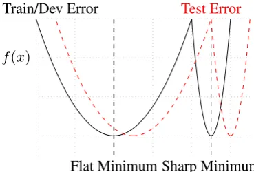
Flat Minimum Sharp Minimum
Train/Dev Error Test Error
[image:2.595.321.506.491.616.2]f(x)
Figure 1: A conceptual sketch of flat and sharp minima from Keskar et al. (2016). The Y-axis indicates values of the error function and the X-axis the weight-space.
a small neighborhood of the minimum. A concep-tual sketch is given inFigure 1. The error functions for training and testing are typically not perfectly synced, i.e. the local minima on the train or devel-opment set are not the local minima for the held-out test set. A sharp minimum usually depicts poorer generalization capabilities, as a slight variation re-sults in a rapid increase of the error function. On the other hand, flat minima generalize better on new data (Keskar et al.,2016). Keskar et al. ob-serve for the MNIST, TIMIT, and CIFAR dataset, that the generalization gap is not due toover-fitting
or over-training, but due to different generaliza-tion capabilities of the local minima the networks converge to.
A priori it is unknown to which type of local mini-mum a neural network will converge. Some meth-ods like the weight initialization (Erhan et al.,2010; Glorot and Bengio,2010) or small-batch training (Keskar et al.,2016) help to avoid bad (e.g. sharp) minima. Nonetheless, the non-deterministic behav-ior of approaches must be considered when they are evaluated.
3 Impact of Randomness in the Evaluation of Neural Networks
Two recent, state-of-the-art systems for NER are proposed byMa and Hovy(2016)5and byLample et al.(2016)6. Lample et al. report anF1-score of
90.94%and Ma and Hovy report anF1-score of
91.21%. Ma and Hovy draw the conclusion that their system achieves a significant improvement over the system by Lample et al.
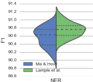
We re-ran both implementations multiple times, each time only changing the seed value of the ran-dom number generator. We ran the Ma and Hovy system 86 times and the Lample et al. system, due to its high computational requirement, for 41 times. The score distribution is depicted as a violin plot inFigure 2. Using a Kolmogorov-Smirnov significance test (Massey, 1951), we observe a statistically significant difference between these two distributions (p < 0.01). The plot reveals that the quartiles for the Lample et al. system are above those of the Ma and Hovy system. Further it reveals a smaller standard deviationσof theF1
-5https://github.com/XuezheMax/ LasagneNLP
6https://github.com/glample/tagger
[image:3.595.340.491.143.277.2]scores for the Lample et al. system. Using a Brown-Forsythe test, the standard deviations are different withp <0.05. Table 1shows the minimum, the maximum, and the median performance for the test performances.
Figure 2: Distribution of scores for re-running the system by Ma and Hovy (left) and Lample et al. (right) multiple times with different seed values. Dashed lines indicate quartiles.
Based on this observation, we draw the conclusion that the system by Lample et al. outperforms the system by Ma and Hovy, as their implementation achieves a higher score distribution and shows a lower standard deviation.
In a usual setup, approaches would be compared on a development set and the run with the highest development score would be used for unseen data, i.e. be used to report the test performance. For the Lample et al. system we observe a Spearman’s rank correlation between the development and the test score ofρ= 0.229. This indicates a weak correla-tion and that the performance on the development set is not a reliable indicator. Using the run with the best development score (94.44%) would yield a test performance of mere90.31%. Using the second best run on development set (94.28%), would yield state-of-the-art performance with91.00%. This dif-ference is statistically significant (p <0.002). In conclusion, a development set will not necessarily solve the issue with bad local minima.
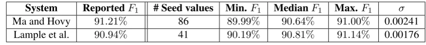
System ReportedF1 # Seed values Min.F1 MedianF1 Max.F1 σ
Ma and Hovy 91.21% 86 89.99% 90.64% 91.00% 0.00241
[image:4.595.77.515.61.108.2]Lample et al. 90.94% 41 90.19% 90.81% 91.14% 0.00176
Table 1: The system by Ma and Hovy(2016) andLample et al.(2016) were run multiple times with different seed values.
Task Dataset # Configs Median Difference 95th percentile Max. Difference
POS Penn Treebank 269 0.17% 0.78% 1.55%
Chunking CoNLL 2000 385 0.17% 0.50% 0.81%
NER CoNLL 2003 406 0.38% 1.08% 2.59%
Entities ACE 2005 405 0.72% 2.10% 8.23%
Events TempEval 3 365 0.43% 1.23% 1.73%
Table 2: The table depicts the median, the 95th percentile and the maximum difference between networks with the same hyperparameters but different random seed values.
statistically significant improvement for the tasks POS, Chunking and Event Detection. For NER and Entity Recognition, the difference was statis-tically not significant given the number of tested hyperparameters.
In the next step, we evaluated the impact of the random seed value for the five sequence tagging tasks described insection 4. We sampled randomly 1830 different configurations, for example different numbers of recurrent units, and ran the network twice, each time with a different seed value. The results are depicted inTable 2.
The largest difference was observed for the ACE 2005 Entities dataset: Using one seed value, the net-work achieved anF1performance of 82.5% while
using another seed value, the network achieved a performance of only 74.3%. Even though this is a rare extreme case, the median difference between different weight initializations is still large. For example for the CoNLL 2003 NER dataset, the me-dian difference is at 0.38% and the 95th percentile is at 1.08%.
In conclusion, if the fact of different local minima is not taken care of and single performance scores are compared, there is a high chance of drawing false conclusions and either rejecting promising approaches or selecting weaker approaches due to a more or less favorable sequence of random numbers.
4 Experimental Setup
In order to find LSTM-network architectures that perform robustly on different tasks, we selected five classical NLP tasks as benchmark tasks: Part-of-Speech tagging (POS), Chunking, Named Entity Recognition (NER), Entity Recognition (Entities) and Event Detection (Events).
For Part-of-Speech tagging, we use the benchmark setup described byToutanova et al.(2003). Using the full training set for POS tagging would hin-der our ability to detect design choices that are consistently better than others. The error rate for this dataset is approximately 3% (Marcus et al., 1993), making all improvements above 97% accu-racy likely the result of chance. A 97.24% accuaccu-racy was achieved byToutanova et al.(2003). Hence, we reduced the training set size from over 38.000 sentences to the first 500 sentences. This decreased the accuracy to about 95%.
For Chunking, we use the CoNLL 2000 shared task setup. For Named Entity Recognition (NER), we use the CoNLL 2003 setup. The ACE 2005 entity recognition task annotated not only named entities, but all words referring to an entity, e.g. the phrase
U.S. president. We use the same data split asLi et al.(2013). For the Event Detection task, we use the TempEval3 Task B setup. There, the smallest extent of text, usually a single word, that expresses the occurrence of an event, is annotated.
4.1 Model
We use a BiLSTM-network for sequence tagging as described in (Huang et al.,2015;Ma and Hovy, 2016;Lample et al.,2016). To be able to evaluate a large number of different network configurations, we optimized our implementation for efficiency, reducing by a factor of 6 the time required per epoch compared toMa and Hovy(2016).
4.2 Evaluated Parameters
We evaluate the following design choices and hy-perparameters:
Pre-trained Word Embeddings. We evaluate the Google News embeddings (G. News)7 from Mikolov et al. (2013), the Bag of Words (Le. BoW) as well as the dependency based embed-dings (Le. Dep.)8 byLevy and Goldberg(2014), three different GloVe embeddings9from Penning-ton et al.(2014) trained either on Wikipedia 2014 + Gigaword 5 (GloVe1with 100 dimensions and
GloVe2 with 300 dimensions) or on Common Crawl (GloVe3), and theKomninos and Manand-har(2016) embeddings (Komn.)10. We also evalu-ate the approach ofBojanowski et al.(2016) ( Fast-Text), which trains embeddings for n-grams with length 3 to 6. The embedding for a word is defined as the sum of the embeddings of the n-grams.
Character Representation. We evaluate the ap-proaches of Ma and Hovy (2016) using Convo-lutional Neural Networks (CNN) as well as the approach of Lample et al. (2016) using LSTM-networks to derive character-based representa-tions.
Optimizer. Besides Stochastic Gradient Descent (SGD), we evaluateAdagrad(Duchi et al.,2011),
Adadelta(Zeiler,2012),RMSProp(Hinton,2012),
Adam(Kingma and Ba,2014), andNadam(Dozat, 2015), an Adam variant that incorporates Nesterov momentum (Nesterov,1983) as optimizers.
Gradient Clipping and Normalization. Two common strategies to deal with the exploding
gradi-7https://code.google.com/archive/p/ word2vec/
8https://levyomer.wordpress.com/2014/ 04/25/dependency-based-word-embeddings/
9http://nlp.stanford.edu/projects/ glove/
10https://www.cs.york.ac.uk/nlp/extvec/
ent problem aregradient clipping(Mikolov,2012) andgradient normalization(Pascanu et al.,2013). Gradient clipping involves clipping the gradient’s components element-wise if it exceeds a defined threshold. Gradient normalization has a better theo-retical justification and rescales the gradient when-ever the norm goes over a threshold.
Tagging schemes. We evaluate the BIO and
IOBESschemes for tagging segments.
Dropout.We compareno dropout,naive dropout, and variational dropout (Gal and Ghahramani, 2016). Naive dropout applies a new dropout mask at every time step of the LSTM-layers. Variational dropout applies the same dropout mask for all time steps in the same sentence. Further, it applies dropout to the recurrent units. We evaluate the dropout rates{0.05,0.1,0.25,0.5}.
Classifier. We evaluate a Softmax classifier as well as a CRF classifier as the last layer of the network.
Number of LSTM-layers.We evaluated1,2, and
3stacked BiLSTM-layers.
Number of recurrent units. For each
LSTM-layer, we selected independently
a number of recurrent units from the set {25,50,75,100,125}.
Mini-batch sizes. We evaluate the mini-batch sizes 1, 8, 16, 32, and 64.
5 Robust Model Evaluation
We have shown insection 3that re-running non-deterministic approaches multiple times and com-paring score distributions is essential to draw cor-rect conclusions. However, to truly understand the capabilities of an approach, it is interesting to test the approach with different sets of hyperparameters for the complete network.
Training and tuning a neural network can be time consuming, sometimes taking multiple days to train a single instance of a network. A priori it is hard to know which hyperparameters will yield the best performance and the selection of the parameters often makes the difference betweenmediocreand
or new languages, as a large range of possible pa-rameters must be evaluated, each time requiring a significant amount of training time. Hence it is desirable, that the approach yields stable results for a wide range of parameters.
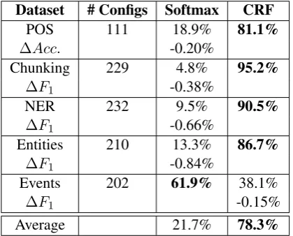
In order to find approaches that result in high per-formance and are robust against the remaining pa-rameters, we decided to randomly sample several hundred network configurations from the set de-scribed insection 4.2. For each sampled configu-ration, we compare different options, e.g. different options for the last layer of the network. For ex-ample, we sampled in total 975 configurations and each configuration was trained with a Softmax clas-sifier as well as with a CRF clasclas-sifier, totaling to 1950 trained networks.
Dataset # Configs Softmax CRF
POS 111 18.9% 81.1%
∆Acc. -0.20%
Chunking 229 4.8% 95.2%
∆F1 -0.38%
NER 232 9.5% 90.5%
∆F1 -0.66%
Entities 210 13.3% 86.7%
∆F1 -0.84%
Events 202 61.9% 38.1%
∆F1 -0.15%
Average 21.7% 78.3%
Table 3: Percentages of configurations where Soft-max or CRF classifiers demonstrated a higher test performance.
Our results are presented in Table 3. The table shows that for the NER task 232 configurations were sampled randomly and for 210 of the 232 configurations (90.5%), the CRF setup achieved a better test performance than the setup with a Soft-max classifier. To measure the difference between these two options, we compute the median of the absolute differences: LetSibe the test performance
(F1-measure) for the Softmax setup for
configura-tion i and Ci the test performance for the CRF
setup. We then compute ∆F1 = median(S1 −
C1, S2−C2, . . . , S232−C232). For the NER task,
the median difference was∆F1 = −0.66%, i.e.
the setup with a Softmax classifier achieved on av-erage anF1-score of 0.66 percentage points below
that of the CRF setup.
We also evaluated the standard deviation of theF1
-scores to detect approaches that are less dependent on the remaining hyperparameters and the random number generator. The standard deviationσfor the CRF-classifier is with 0.0060 significantly lower (p <10−3using Brown-Forsythe test) than for the
Softmax classifier withσ= 0.0082.
6 Results
This section highlights our main insights in the evaluation of different design choices for BiL-STM architectures. We limit the number of results we present for reasons of brevity. Detailed infor-mation can be found in (Reimers and Gurevych, 2017).11
[image:6.595.77.287.295.464.2]6.1 Classifier
Table 3shows a comparison between using a Soft-max classifier as a last layer and using a CRF classi-fier. The BiLSTM-CRF architecture byHuang et al. (2015) achieves a better performance on 4 out of 5 tasks. For the NER task it further achieves a 27% lower standard deviation (statistically significant withp <10−3), indicating that it is less sensitive to
the remaining configuration of the network. The CRF classifier only fails for the Event Detec-tion task. This task has nearly no dependency be-tween tags, as often only a single token is annotated as an event trigger in a sentence.
We studied the differences between these two clas-sifiers in terms of number of LSTM-layers. As Figure 3shows, a Softmax classifier profits from a deep LSTM-network with multiple stacked lay-ers. On the other hand, if a CRF classifier is used, the effect of additional LSTM-layers is much smaller.
6.2 Optimizer
We evaluated six optimizers with the suggested default configuration from their respective papers. We observed that SGD is quite sensitive towards the selection of the learning rate and it failed in many instances to converge. For the optimizers SGD, Adagrad and Adadelta we observed a large standard deviation in terms of test performance,
11https://public.ukp.informatik. tu-darmstadt.de/reimers/Optimal_
Figure 3: Difference between Softmax and CRF classifier for different number of BiLSTM-layers for the CoNLL 2003 NER dataset.
which was for the NER task at 0.1328 for SGD, 0.0139 for Adagrad, and 0.0138 for Adadelta. The optimizers RMSProp, Adam, and Nadam on the other hand produced much more stable results. Not only were the medians for these three optimizers higher, but also the standard deviation was with 0.0096, 0.0091, and 0.0092 roughly 35% smaller in comparison to Adagrad. A large standard devia-tion indicates that the optimizer is sensitive to the hyperparameters as well as to the random initializa-tion and bears the risk that the optimizer produces subpar results.
The best result was achieved by Nadam. For 453 out of 882 configurations (51.4%), it yielded the highest performance out of the six tested optimiz-ers. For the NER task, it produced on average a 0.82 percentage points better performance than Adagrad.
Besides test performance, the convergence speed is important in order to reduce training time. Here, Nadam had the best convergence speed. For the NER dataset, Nadam converged on average after 9 epochs, whereas SGD required 42 epochs.
6.3 Word Embeddings
The pre-trained word embeddings had a large im-pact on the performance as shown in Table 4. The embeddings by Komninos and Manandhar (2016) resulted in the best performance for the POS, the Entities and the Events task. For the Chunking task, the dependency-based embeddings ofLevy and Goldberg(2014) are slightly ahead of the Komninos embeddings, the significance level
is atp= 0.025. For NER, the GloVe embeddings trained on common crawl perform on par with the Komninos embeddings (p= 0.391).
We observe that the underlying word embeddings have a large impact on the performance for all tasks. Well suited word embeddings are especially critical for datasets with small training sets. For the POS task we observe a median difference of 4.97% be-tween the Komninos embeddings and the GloVe2 embeddings.
Note we only evaluated the pre-trained embeddings provided by different authors, but not the underly-ing algorithms to generate these embeddunderly-ings. The quality of word embeddings depends on many fac-tors, including the size, the quality, and the prepro-cessing of the data corpus. As the corpora are not comparable, our results do not allow concluding that one approach is superior for generating word embeddings.
6.4 Character Representation
We evaluate the approaches ofMa and Hovy(2016) using Convolutional Neural Networks (CNN) as well as the approach ofLample et al.(2016) using LSTM-networks to derive character-based repre-sentations.
Dataset Le. Dep. Le. BoW GloVe1 GloVe2 GloVe3 Komn. G. News FastText
POS 6.5% 0.0% 0.0% 0.0% 0.0% 93.5% 0.0% 0.0%
∆Acc. -0.39% -2.52% -4.14% -4.97% -2.60% -1.95% -2.28%
Chunking 60.8% 0.0% 0.0% 0.0% 0.0% 37.1% 2.1% 0.0%
∆F1 -0.52% -1.09% -1.50% -0.93% -0.10% -0.48% -0.75%
NER 4.5% 0.0% 22.7% 0.0% 43.6% 27.3% 1.8% 0.0%
∆F1 -0.85% -1.17% -0.15% -0.73% -0.08% -0.75% -0.89%
Entities 4.2% 7.6% 0.8% 0.0% 6.7% 57.1% 21.8% 1.7%
∆F1 -0.92% -0.89% -1.50% -2.24% -0.80% -0.33% -1.13%
Events 12.9% 4.8% 0.0% 0.0% 0.0% 71.8% 9.7% 0.8%
∆F1 -0.55% -0.78% -2.77% -3.55% -2.55% -0.67% -1.36%
[image:8.595.321.511.285.455.2]Average 17.8% 2.5% 4.7% 0.0% 10.1% 57.4% 7.1% 0.5%
Table 4: Randomly sampled configurations were evaluated with 8 possible word embeddings. 108 configurations were sampled for POS, 97 for Chunking, 110 for NER, 119 for Entities, and 124 for Events.
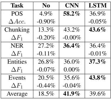
The difference between the CNN approach byMa and Hovy(2016) and the LSTM approach by Lam-ple et al.(2016) to derive a character-based repre-sentations is statistically insignificant for all tasks. This is quite surprising, as both approaches have fundamentally different properties: The CNN ap-proach fromMa and Hovy(2016) takes only tri-grams into account. It is also position independent, i.e. the network will not be able to distinguish be-tween trigrams at the beginning, in the middle, or at the end of a word, which can be crucial information for some tasks. The BiLSTM approach from Lam-ple et al.(2016) takes all characters of the word into account. Further, it is position aware, i.e. it can distinguish between characters at the start and at the end of the word. Intuitively, one would think that the LSTM approach by Lample et al. would be superior.
6.5 Gradient Clipping and Normalization
Forgradient clipping(Mikolov,2012) we couldn’t observe any improvement for the thresholds of 1, 3, 5, and 10 for any of the five tasks.
Gradient normalizationhas a better theoretical jus-tification (Pascanu et al.,2013) and we can confirm with our experiments that it performs better. Not normalizing the gradient was the best option only for 5.6% of the 492 evaluated configurations (un-der null-hypothesis we would expect 20%). Which threshold to choose, as long as it is not too small or too large, is of lower importance. In most cases, a threshold of 1 was the best option (30.5% of the
Task No CNN LSTM
POS 4.9% 58.2% 36.9%
∆Acc. -0.90% -0.05%
Chunking 13.3% 43.2% 43.6%
∆F1 -0.20% -0.00%
NER 27.2% 36.4% 36.4%
∆F1 -0.11% -0.01%
Entities 26.8% 36.0% 37.3%
∆F1 -0.07% 0.00%
Events 20.5% 35.6% 43.8%
∆F1 -0.44% -0.04%
Average 18.5% 41.9% 39.6%
Table 5: Comparison of not using character-based representations and using CNNs (Ma and Hovy, 2016) or LSTMs (Lample et al.,2016) to derive character-based representations. 225 configura-tions were sampled for POS, 241 for Chunking, 217 for NER, 228 for Entities, and 219 for Events.
cases).
We observed a large performance increase com-pared to not normalizing the gradient. The median increase was between 0.29 percentage pointsF1
-score for the Chunking task and 0.82 percentage points for the POS task.
6.6 Dropout
op-tion in 83.5% of the 479 evaluated configuraop-tions. The median performance increase in comparison to not using dropout was between 0.31 percentage points for the POS-task and 1.98 for the Entities task. We also observed a large improvement in comparison to naive dropout between 0.19 percent-age points for the POS task and 1.32 percentpercent-age points for the Entities task. Variational dropout showed the smallest standard deviation, indicating that it is less dependent on the remaining hyperpa-rameters and the random number sequence. We further evaluated whether variational dropout should be applied to the output units of the LSTM-network, to the recurrent units, or to both. We observed that applying dropout to both dimensions gave in most cases (62.6%) the best results. The me-dian performance increase was between 0.05 per-centage points and 0.82 perper-centage points.
6.7 Further Evaluated Parameters
The tagging schemesBIOandIOBESperformed on par for 4 out of 5 tasks. For the Entities task, theBIOscheme significantly outperformed the IOBES scheme for 88.7% of the tested con-figurations. The median difference was ∆F1 =
−1.01%.
For the evaluated tasks, 2 stacked LSTM-layers achieved the best performance. For the POS-tagging task, 1 and 2 layers performed on par. For flat networks with a single LSTM-layer, around 150 recurrent units yielded the best performance. For networks with 2 or 3 layers, around 100 recurrent units per network yielded the best performance. However, the impact of the number of recurrent units was extremely small.
For tasks with small training sets, smaller mini-batch sizes of 1 up to 16 appears to be a good choice. For larger training sets sizes of 8 - 32 appears to be a good choice. Mini-batch sizes of 64 usually performed worst.
7 Conclusion
In this paper, we demonstrated that the sequence of random numbers has astatistically significant im-pact on the test performance and that wrong conclu-sions can be made if performance scores based on single runs are compared. We demonstrated this for the two recent state-of-the-art NER systems byMa
and Hovy(2016) andLample et al.(2016). Based on the published performance scores, Ma and Hovy draw the conclusion of a significant improvement over the approach of Lample et al. Re-executing the provided implementations with different seed values however showed that the implementation of Lample et al. results in a superior score distribution generalizing better to unseen data.
Comparing score distributions reduces the risk of rejecting promising approaches or falsely accepting weaker approaches. Further it can lead to new in-sights on the properties of an approach. We demon-strated this for ten design choices and hyperparam-eters of LSTM-networks for five tasks.
By studying the standard deviation of scores, we estimated the dependence on hyperparameters and on the random seed value for different approaches. We showed that SGD, Adagrad and Adadelta have a higher dependence than RMSProp, Adam or Nadam. We have shown that variational dropout also reduces the dependence on the hyperparame-ters and on the random seed value. As future work, we will investigate if those methods are either less dependent on the hyperparameters or are less de-pendent on the random seed value, e.g. if they avoid converging to bad local minima.
By testing a large number of configurations, we showed that some choices consistently lead to su-perior performance and are less dependent on the remaining configuration of the network. Thus, there is a good chance that these configurations require less tuning when applied to new tasks or domains.
Acknowledgements
References
Daniel Andor, Chris Alberti, David Weiss, Aliaksei Severyn, Alessandro Presta, Kuzman Ganchev, Slav Petrov, and Michael Collins. 2016. Globally
nor-malized transition-based neural networks. CoRR,
abs/1603.06042.
Piotr Bojanowski, Edouard Grave, Armand Joulin,
and Tomas Mikolov. 2016. Enriching Word
Vec-tors with Subword Information. arXiv preprint
arXiv:1607.04606.
Timothy Dozat. 2015. Incorporating Nesterov Momen-tum into Adam.
John Duchi, Elad Hazan, and Yoram Singer. 2011. Adaptive Subgradient Methods for Online Learning
and Stochastic Optimization. J. Mach. Learn. Res.,
12:2121–2159.
Dumitru Erhan, Yoshua Bengio, Aaron Courville, Pierre-Antoine Manzagol, Pascal Vincent, and Samy Bengio. 2010. Why Does Unsupervised Pre-training
Help Deep Learning? Journal of Machine Learning
Research, 11:625–660.
Antske Fokkens, Marieke van Erp, Marten Postma, Ted Pedersen, Piek Vossen, and Nuno Freire. 2013. Off-spring from Reproduction Problems: What Replication
Failure Teaches Us. InACL (1), pages 1691–1701. The
Association for Computer Linguistics.
Yarin Gal and Zoubin Ghahramani. 2016. A Theoret-ically Grounded Application of Dropout in Recurrent
Neural Networks. InAdvances in Neural Information
Processing Systems 29: Annual Conference on Neural Information Processing Systems 2016, December 5-10, 2016, Barcelona, Spain, pages 1019–1027.
Xavier Glorot and Yoshua Bengio. 2010. Understand-ing the difficulty of trainUnderstand-ing deep feedforward neural
networks. InIn Proceedings of the International
Con-ference on Artificial Intelligence and Statistics (AIS-TATS10). Society for Artificial Intelligence and Statis-tics.
Geoffrey Hinton. 2012. Neural Networks for Machine Learning - Lecture 6a - Overview of mini-batch gradi-ent descgradi-ent.
Sepp Hochreiter and J¨urgen Schmidhuber. 1997a. Flat
Minima.Neural Computation, 9(1):1–42.
Sepp Hochreiter and J¨urgen Schmidhuber. 1997b.
Long Short-Term Memory. Neural Computation,
9(8):1735–1780.
Zhiheng Huang, Wei Xu, and Kai Yu. 2015. Bidi-rectional LSTM-CRF Models for Sequence Tagging.
CoRR, abs/1508.01991.
Frank Hutter, Holger Hoos, and Kevin Leyton-Brown. 2014. An Efficient Approach for Assessing
Hyperpa-rameter Importance. InProceedings of the 31st
Inter-national Conference on InterInter-national Conference on Machine Learning - Volume 32, ICML’14, pages I– 754–I–762. JMLR.org.
Nitish Shirish Keskar, Dheevatsa Mudigere, Jorge No-cedal, Mikhail Smelyanskiy, and Ping Tak Peter Tang.
2016. On Large-Batch Training for Deep
Learn-ing: Generalization Gap and Sharp Minima. CoRR,
abs/1609.04836.
Diederik P. Kingma and Jimmy Ba. 2014. Adam:
A Method for Stochastic Optimization. CoRR,
abs/1412.6980.
Alexandros Komninos and Suresh Manandhar. 2016. Dependency based embeddings for sentence
classifi-cation tasks. In Proceedings of the 2016 Conference
of the North American Chapter of the Association for Computational Linguistics: Human Language Tech-nologies, pages 1490–1500, San Diego, California. As-sociation for Computational Linguistics.
Guillaume Lample, Miguel Ballesteros, Sandeep Sub-ramanian, Kazuya Kawakami, and Chris Dyer. 2016. Neural architectures for named entity recognition.
CoRR, abs/1603.01360.
Y. LeCun, B. Boser, J. S. Denker, D. Henderson, R. E. Howard, W. Hubbard, and L. D. Jackel. 1989. Back-propagation Applied to Handwritten Zip Code
Recog-nition.Neural Computation, 1(4):541–551.
Yann LeCun, L´eon Bottou, Genevieve B. Orr, and Klaus-Robert M¨uller. 1998. Efficient BackProp. In Neural Networks: Tricks of the Trade, This Book is an Outgrowth of a 1996 NIPS Workshop, pages 9–50, Lon-don, UK, UK. Springer-Verlag.
Omer Levy and Yoav Goldberg. 2014.
Dependency-Based Word Embeddings. InProceedings of the 52nd
Annual Meeting of the Association for Computational Linguistics, ACL 2014, June 22-27, 2014, Baltimore, MD, USA, Volume 2: Short Papers, pages 302–308. Qi Li, Heng Ji, and Liang Huang. 2013. Joint Event Ex-traction via Structured Prediction with Global Features. InProceedings of the 51st Annual Meeting of the Asso-ciation for Computational Linguistics (Volume 1: Long Papers), pages 73–82, Sofia, Bulgaria. Association for Computational Linguistics.
Xuezhe Ma and Eduard H. Hovy. 2016. End-to-end Se-quence Labeling via Bi-directional LSTM-CNNs-CRF.
CoRR, abs/1603.01354.
Mitchell P. Marcus, Mary Ann Marcinkiewicz, and Beatrice Santorini. 1993. Building a Large Annotated
Corpus of English: The Penn Treebank. Comput.
Lin-guist., 19(2):313–330.
Frank J. Massey. 1951. The kolmogorov-smirnov test for goodness of fit.Journal of the American Statistical Association, 46(253):68–78.
Tom´aˇs Mikolov. 2012. Statistical language models
based on neural networks. Ph.D. thesis, Brno Univer-sity of Technology.
Yurii Nesterov. 1983. A method of solving a convex programming problem with convergence rate
O(1/sqr(k)). Soviet Mathematics Doklady, 27:372–
376.
Razvan Pascanu, Tomas Mikolov, and Yoshua Bengio. 2013. On the Difficulty of Training Recurrent Neural
Networks. In Proceedings of the 30th International
Conference on International Conference on Machine Learning - Volume 28, ICML’13, pages III–1310–III– 1318. JMLR.org.
Jeffrey Pennington, Richard Socher, and Christopher D. Manning. 2014. Glove: Global vectors for word
repre-sentation. InEmpirical Methods in Natural Language
Processing (EMNLP), pages 1532–1543.
Nils Reimers and Iryna Gurevych. 2017. Optimal Hy-perparameters for Deep LSTM-Networks for Sequence Labeling Tasks. arXiv preprint arXiv:1707.06799. Anders Søgaard and Yoav Goldberg. 2016. Deep multi-task learning with low level multi-tasks supervised at lower
layers. InProceedings of the 54th Annual Meeting of
the Association for Computational Linguistics (Volume 2: Short Papers), pages 231–235, Berlin, Germany. As-sociation for Computational Linguistics.
Nitish Srivastava, Geoffrey Hinton, Alex Krizhevsky, Ilya Sutskever, and Ruslan Salakhutdinov. 2014. Dropout: A Simple Way to Prevent Neural Networks
from Overfitting. J. Mach. Learn. Res., 15(1):1929–
1958.
Kristina Toutanova, Dan Klein, Christopher D. Man-ning, and Yoram Singer. 2003. Feature-rich Part-of-speech Tagging with a Cyclic Dependency Network. In Proceedings of the 2003 Conference of the North Amer-ican Chapter of the Association for Computational Lin-guistics on Human Language Technology - Volume 1, NAACL 2003, pages 173–180, Stroudsburg, PA, USA. Association for Computational Linguistics.
Yonghui Wu, Mike Schuster, Zhifeng Chen, Quoc V. Le, Mohammad Norouzi, Wolfgang Macherey, Maxim Krikun, Yuan Cao, Qin Gao, Klaus Macherey, Jeff Klingner, Apurva Shah, Melvin Johnson, Xiaobing Liu, Lukasz Kaiser, Stephan Gouws, Yoshikiyo Kato, Taku Kudo, Hideto Kazawa, Keith Stevens, George Kurian, Nishant Patil, Wei Wang, Cliff Young, Jason Smith, Ja-son Riesa, Alex Rudnick, Oriol Vinyals, Greg Corrado, Macduff Hughes, and Jeffrey Dean. 2016. Google’s Neural Machine Translation System: Bridging the Gap
between Human and Machine Translation. CoRR,
abs/1609.08144.