258
Interpreting Word-Level Hidden State Behaviour of Character-Level
LSTM Language Models
Avery Hiebert†∗, Cole Peterson†, Alona Fyshe‡, Nishant A. Mehta†
†Department of Computer Science, University of Victoria, Canada ‡Computing Science / Psychology Departments, University of Alberta, Canada
[email protected], [email protected] [email protected], [email protected]
Abstract
While Long Short-Term Memory networks (LSTMs) and other forms of recurrent neural network have been successfully applied to lan-guage modeling on a character level, the hid-den state dynamics of these models can be difficult to interpret. We investigate the hid-den states of such a model by using the HDB-SCAN clustering algorithm to identify points in the text at which the hidden state is similar. Focusing on whitespace characters prior to the beginning of a word reveals interpretable clus-ters that offer insight into how the LSTM may combine contextual and character-level infor-mation to identify parts of speech. We also introduce a method for deriving word vectors from the hidden state representation in order to investigate the word-level knowledge of the model. These word vectors encode meaning-ful semantic information even for words that appear only once in the training text.
1 Introduction
Recurrent Neural Networks (RNNs), including Long Short-Term Memory (LSTM) networks (Hochreiter and Schmidhuber, 1997;Gers et al.,
2000), have been widely applied to natural lan-guage processing tasks including character-level language modeling (Mikolov et al.,2012;Graves,
2013). However, like other types of neural net-works, the hidden states and behaviour of a given LSTM can be difficult to understand and interpret, due to both the distributed nature of the hidden state representations and the relatively opaque re-lationship between the hidden state and the final output of the network. It is also not clear how a character-level LSTM language model takes ad-vantage of orthographic patterns to infer higher-level information.
∗
Corresponding author
In this paper, we investigate the hidden state dy-namics of a character-level LSTM language model both directly and — through the use of output gate activations — indirectly. As an overview, our main contributions are:
1. We use clustering to investigate similar hid-den states (and output gate activations) at dif-ferent points in a text, paying special atten-tion to whitespace characters. We provide in-sight into the model’s awareness of both or-thographic patterns and word-level grammat-ical information.
2. Inspired by our findings from clustering, we introduce a method for extracting meaning-ful word embeddings from a character-level model, allowing us to investigate the word-level knowledge of the model.
First, we use the HDBSCAN clustering algo-rithm (Campello et al., 2013) to reveal locations within a text at which the hidden state of the LSTM is similar, or at which a similar combina-tion of cell state dimensions is relevant (as deter-mined by output gates). Interestingly, focusing on moments when the network must predict the first letter of a word reveals clusters that are in-terpretable on the level of words and which dis-play both character-level patterns and grammati-cal structure (i.e. separating parts of speech). We give examples of clusters of similar hidden states that appear to be heavily influenced by local ortho-graphic patterns but also distinguish between dif-ferent grammatical functions of the pattern — for example, a cluster containing whitespace charac-ters following possessive uses, but not contractive uses, of the affix “’s”. This sheds light on the use of orthographic patterns to infer higher-level infor-mation.
embeddings from a character-level model and per-form qualitative and quantitative analyses of these embeddings. Surprisingly, this method can as-sign meaningful representations even to words that appear only once in the text, including associ-ating the rare word “scrutinizingly” with “ques-tioningly” and “attentively”, and correctly iden-tifying “deck” as a verb based on a single use despite its lack of meaningful subword compo-nents. These results suggests that the model is ca-pable of deducing meaningful information about a word based on the context of a single use. While these embeddings do not achieve state-of-the-art performance on word similarity benchmarks, they do outperform the older methods of Turian et al.
(2010) despite the small corpus size and the fact that our language model was not designed with the intent of producing word embeddings.
The rest of the paper is structured as follows: The following section describes related work. Sec-tion3describes the architecture and training of the LSTM language model used in our experiments. In Section4, we describe our clustering methods and show examples of the clusters found, as well as a part of speech analysis. In Section5, we de-scribe and analyze our method for extracting word embeddings from the character-level model. Fi-nally, we conclude and suggest directions for fu-ture work.
2 Related Work
2.1 Analyzing Hidden State Dynamics
Many researchers have investigated techniques for understanding the meaning and dynamics of the hidden states of recurrent neural networks. In his seminal paper (Elman, 1990) introducing the simple recurrent network (SRN) (or “Elman net-work”), Elman uses hierarchical clustering to in-vestigate the hidden states of a word-level RNN modeling a toy language of 29 words. Our ap-proach in Section 4 is in some ways similar, al-though we use real English data and a character-level LSTM model. This also bears some similari-ties to a visualization technique used byKrakovna and Doshi-Velez (2016) to investigate a hybrid HMM-LSTM model, although their work uses only 10 k-means clusters and does not deeply in-vestigate clustering. Elman also uses principal component analysis to visualize hidden state over time (1991), and many researchers have used di-mensionality reduction methods such as t-SNE
(Van der Maaten and Hinton, 2008) to visualize similarity between word embeddings, as well as other forms of distributed representation. More recently,Li et al. (2016) directly visualize repre-sentations over time using heatmaps, andStrobelt et al.(2018) develop interactive tools for visual-izing LSTM hidden states and testing hypotheses about distributed representations.
Other researchers have investigated methods for clarifying the function of specific hidden dimen-sions. Karpathy et al. (2015) use static visu-alizations to demonstrate the existence of cells in an LSTM language model with interpretable behaviour representing long-term dependencies (such as cells tracking line length or quotations in a text). Another approach is that of K´ad´ar et al.(2017), who introduce a “Top K Contexts” method for interpreting the function of certain hid-den dimensions, ihid-dentifying theK points in a se-quence which experience the highest activations for the dimension in question.
2.2 Character-Level Word Embeddings
Multiple researchers have developed methods for creating word embeddings that incorporate sub-word level (Luong et al.,2013) or character-level (Santos and Zadrozny,2014;Ling et al.,2015) in-formation in order to better handle rare or out-of-vocabulary words. These approaches differ from our work in Section 5 in that they use architec-tures specifically designed to create word embed-dings, while we create embeddings from the hid-den state of a character-level model not designed for this purpose. In addition, we are interested not in the embeddings themselves, but rather in what they tell us about the word-level knowledge of the language model.
Kim et al.(2016) investigate word embeddings created by a character-aware language model; however, the model uses word-level inputs that are further subdivided into character-level information and makes predictions on the word level, while we use an entirely character-level model.
3 Model
In this paper we focus on the task of language modeling on the character level. Given an input se-quence of characters, the model is tasked with pre-dicting the log probability of the following charac-ter.
us-ing the same architecture. Most of the paper fo-cuses on the War and Peace model, but Section
5 uses embeddings derived from the Lancaster-Oslo/Bergen Corpus model when measuring per-formance against word embedding benchmarks.
3.1 Training Data
Our first model uses a relatively small data set, consisting of the text of War and Peace by Tol-stoy1. This data set was chosen due to its conve-nience as a sufficiently long but stylistically con-sistent example of English text. The text contains 3,201,616 characters. We use the first 95% of the data for training and the last 5% for validation.
Our second model uses a slightly larger data set, consisting of the Lancaster-Oslo/Bergen (LOB) corpus (Johansson et al., 1978)2, which we re-moved all markup from. This data set draws from a wide variety of fiction and non-fiction texts written in British English in 1961, and contains 5,818,332 characters total. It was chosen for use in Section5because it covers a wide range of top-ics (allowing us to extract word embeddings for a wider vocabulary) while still remaining at a man-ageable size. We use the last 95% of the data for training and the first 5% for validation.
3.2 Model Architecture and Implementation
We use a simple LSTM architecture consisting of a 256-dimensional character embedding layer, followed by three 512-dimensional LSTM layers, and a final layer producing a log softmax distribu-tion over the set of possible characters. The model was implemented in PyTorch (Paszke et al.,2017) using the default LSTM implementation3.
This architecture was chosen mostly arbitrarily, and distantly inspired byKarpathy et al.(2015).
3.3 Training
The War and Peace model was trained for 170 epochs using stochastic gradient descent and the negative log likelihood loss function, with mini-batches of size 100 and truncated backpropaga-tion through time (BPTT) of 100 time steps. Dur-ing trainDur-ing, dropout was applied after each LSTM layer with a dropout rate of 0.5. The learning rate
1
(Tolstoy, 2009), translated to English by Louise and Aylmer Maude.
2
retrieved from http://purl.ox.ac.uk/ota/ 0167
3We intend to release our code, including the trained
mod-els.
was initially set to 1 and halved every time the loss on the validation data set plateaued. The final model achieved 1.660 bits-per-character (BPC) on the validation data.
The Lancaster-Oslo/Bergen model was trained for 100 epochs using the PyTorch implementation of AdaGrad, with mini-batches of size 100, trun-cated BPTT of 100 time steps, a dropout rate of 0.5, and an initial learning rate of 0.01.4 The final model achieved 1.787 BPC on the validation data.
4 Cluster Analysis of Character-Level and Word-Level Patterns
In this section we analyze points in the training text by clustering according to hidden state val-ues and output gate activations, revealing a combi-nation of grammatical and word-level patterns re-flected in the hidden state of our language model.
4.1 Data For Clustering
We created two sets of data for use in clustering: a “full” data set and a “whitespace” data set.
To create the “full” data set, we ran ourWar and Peacelanguage model on the first 50,000 charac-ters5of the training data and recorded the hidden state (i.e. the values often denotedhtin the LSTM literature, rather than the cell statect) and the sig-moid activations of the output gate of the third LSTM layer at each time step. We focus on the third layer based on the expectation that it will en-code more high-level information than earlier lay-ers, an expectation which was supported by brief experimentation on the first layer.
To create the “whitespace” data set, we ran the War and Peacemodel on the first 250,000 charac-ters of the training data and recorded data only for timesteps when the input character was a space or a new line character.
4.2 Basic Clustering Experiment
We chose to use the HDBSCAN clustering algo-rithm (Campello et al.,2013), since it is designed to work with non-globular clusters of varying den-sity, does not require that an expected number of clusters be specified in advance, and is willing to avoid assigning points to a cluster if they do not
4Training parameters were not tuned to the data and differ
mainly because the models were not trained at the same time, with unrelated experiments intervening.
5This smaller data set was used due to the relatively
Cluster Sample Cluster Members
4
even wi[s]h to; conversing wi[t]h; case wi[t]h; whi[c]h was; him wi[t]h; his wi[f]e; very wi[t]ty; acts whi[c]h;
7
so[m]ething like; she sa[w] that; Hardenburg sa[y]s; the sa[m]e time; none se[e]med to; words su[g]gested.
14 e[x]plains; e[v]erything; e[x]posed; e[x]pectations; e[l]derly; e[x]pression;
39 thi[s] reception; tha[t] profound; like thi[s]?”; the[y] promised; the[y] have; The[r]e is;
54
who[ ]is; He[ ]spoke; he[ ]indicated; who[ ]had; He[ ]frowned; She[ ]was; who[ ]was; she[ ]said; why[ ]he
56
on[ ]the; for[ ]God’s; of[ ]the; of[ ]them; by[ ]imbecility; for[ ]Pierre; of[ ]young people; from[ ]abroad;
62
had[ ]gone; had[ ]the; had[ ]been; have[ ]reference; have[ ]promised; had[ ]also; has[ ]been; has[ ]to;
63
her[ ]house; that[ ]is; his[ ]boats;
[image:4.595.72.292.59.296.2]this[ ]pretty; that[ ]this; prevented her[ ]from; her[ ]age; his[ ]way; her[ ]duties;
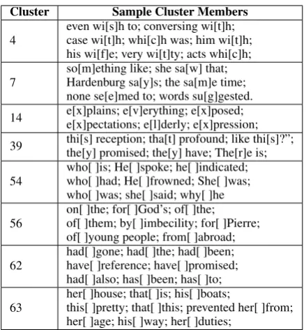
Table 1: Example members of clusters found using hidden state values based on the “full” data set. Cluster members (indicated by brackets) are accompanied by text excerpts (separated by semicolons) to give context.
seem to be a good fit for any cluster. We used the Python implementation ofMcInnes et al.(2017).
Using the “full” data set, we attempted to cluster the time steps according to either hid-den state or output gate activations. We used the Euclidean metric and the HDBSCAN param-eters min cluster size=100 and min samples=10. This was chosen somewhat arbitrarily and not on the basis of a parameter search; we did briefly try other settings during preliminary research and found that the results were similar6. Clustering by hidden state values and clustering by output gate activations both produced a number of inter-pretable clusters7.
Table 1 shows a representative sample of the clusters found when using the hidden state for clustering8. We found that most clusters seemed to have interpretable meanings on the character level, often including characters near the start of words that begin with a particular character or characters, as in clusters 4, 7, and 14. In some cases, these clusters seem to locate orthographic patterns that
6
Of course, allowing smaller clusters results in more clus-ters, while requiring larger clusters results in fewer, broader clusters, but there were no major qualitative differences in the types of clusters produced.
7
Clustering by hidden state produced 67 clusters, while clustering by output gate activations produced 87 clusters.
8The output gate clusters were similar and are omitted to
save space.
are useful in predicting the following character; for example, the characters in cluster 4 are often followed by an “h”, and cluster 39 contains mostly letters at the end of a word (i.e. usually followed by whitespace). However, we did not find clusters that were characterised only by the following char-acters and not by patterns in the preceding charac-ters.
More interestingly, clusters consisting of points immediately preceding the start of a word tended to reflect word-level information relating to the preceding word. For example, cluster 54 con-sists of spaces immediately following the pro-nouns “he” and “she”, as well as the interroga-tive pronoun “who”9, while cluster 56 consists of spaces following certain prepositions. This was observed in both the clusters based on hidden state and the clusters based on output gate activation. This could be due to the fact that the output gate activations, which also impact the hidden state, can be intepreted as choosing which dimensions of the cell state are relevant for the network’s “de-cision” at a given time, and we would expect that word-level information is relevant when choosing a distribution over the first letter of the next word.
4.3 Whitespace Clustering and Part-of-Speech Analysis
Since the clusters including whitespace tended to reflect word-level grammatical information (as seen in clusters 54, 56, and 62 from Table1), we performed another round of clustering restricting our focus to only spaces and new lines. Cluster-ing was performed on the “whitespace” data ac-cording to either hidden states or output gate acti-vations, again producing many interpretable clus-ters10.
For the purposes of word-level analysis, each data point (corresponding to a whitespace charac-ter in the text) was equated with the word imme-diately preceding it. The Stanford Part-of-Speech Tagger (Toutanova et al., 2003) was used to tag the text with part of speech (POS) information, and for each cluster theprecision (percentage of words in the cluster having a given tag) and re-call(percentage of words with a given tag falling
9This cluster also occasionally includes spaces following
the word “why”, which may be due to orthographic similarity to “who”, or due to the fact that “why” is often followed by a verb, as in “Why is...”.
10Clustering by hidden states produced 70 clusters, while
Cluster Sample Members of Cluster POS - Precision POS - Recall
HS-35 asked; replied; remarked; continued; replied; cried; cried;
repeated; continued; exclaimed; remarked; remarked; continued; declared; VBD: 100% VBD: 4.5%
HS-40
will; will; don’t; don’t; don’t; cannot; just; can’t; will; will; might; could; shall; will; would; just; would; just; just; don’t; don’t; could;
MD: 59.2% RB: 18.3% NN: 21.3%11
MD: 89.9% RB: 5.1% NN: 2.9%
HS-57 looking; looked; looking; looked; looked; looking; walked; glanced; looking; looking; glancing; looked; looked; looked; looking
VBD: 60.0% VBG: 40.0%
VBD: 2.4% VBG: 4.8%
HS-59
trembled; jumped; tucked; smoothed; smiled; raised; standing; smiled; pushed; smiled; passed; crowding; turning; raised; climbed; watched; turned; changed;
VBD: 59.1% VBG: 31.5% VBN: 8.7%
VBD: 6.0% VBG: 9.7% VBN: 3.3%
HS-62
unnatural; beautiful; beautiful; beautiful; terrified;
suppressed; proud-looking; polished; well-garnished; nice-looking; swaggering; wonderful; embittered; alarmed; mournful
JJ: 84.4% VBN: 6.7% VBG: 4.4%
JJ: 4.1% VBN: 0.9% VBG: 0.5%
OG-69
laughter; mother; father; daughter; father; father; matter; daughter; father; manner; officer; father; daughter; mother; laughter; daughter; daughter; father; officer;
NN: 94.1% NNS: 2.9% JJ: 2.9%
NN: 1.9% NNS: 0.3% JJ: 0.1%
OG-74 emancipation; nation; conversation; conversation; opinion conversation; resignation; conversation; conversation; expression;
NN: 95.7% NNP: 4.4%
[image:5.595.73.530.60.259.2]NN: 3.8% NNP: 0.3%
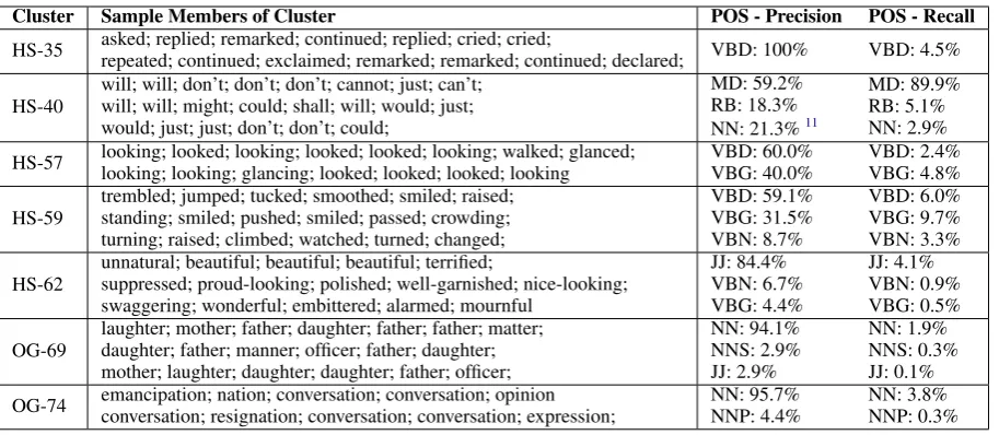
Table 2: Cluster members and POS statistics. Example cluster members (corresponding to whitespace characters) are drawn uniformly at random from the cluster and are represented by the preceding word. Note that some words appear multiple times since each appearance of the word in the text corresponds to a different data point. POS tags are those used by the Stanford POS tagger. Statistics are reported for the three parts of speech with highest precision.
into the cluster)12 were calculated with respect to each tag. Since the clusters are based only on data corresponding to whitespace, words not followed by whitespace (approximately 16% of all words) were not counted when calculating recall.
A selection of clusters, example members, and POS statistics can be seen in Table2. Clusters are designated “OG” or “HS” for “output gate” and “hidden state” respectively, so “HS-35” means the 35th cluster produced when clustering by hidden state values. These clusters were selected to illus-trate the interesting patterns present, rather than to represent “typical” clusters.
The resulting clusters based on hidden states were similar to those based on output gate acti-vations. Both approaches resulted in some clus-ters based on a mix of orthographic and semantic similarity — for example, both produced a clus-ter consisting primarily of three-letclus-ter verbs be-ginning with “s” (particularly “sat”, “saw”, and “say”), as well as clusters consisting of possessive uses of the suffix “’s”, but not uses of “’s” as a contraction of “is” (as in “it’s”, “that’s”, etc.), de-spite the existence of several such uses in the text.
11Manual inspection suggests that the claimed 22%
preci-sion for nouns is actually due to the POS tagger mistaking “don’t”, “can’t” etc. for nouns, probably due to poor tok-enization, meaning that the true precision for modal verbs in this cluster is 80% if we consider these to be modal verbs.
12Note that when measured in this way, recall will usually
be quite low, since most clusters only contain some particular subset of words with a given tag.
In fact, some early experimentation resulted in a distinct cluster for the contractive use of “’s”, al-though this does not occur with the parameters we chose for our canonical data. Additionally, in both cases the majority of clusters contained instances of only a single word or a small set of words — for example, a cluster consisting entirely of the word “the”, a cluster consisting almost entirely of the words “he” and “she”, and a cluster containing only the words “me” and “my”. In total, 71% of clusters either contained only one or two words, or were determined by preceding punctuation.
However, there were qualitative differences be-tween the two approaches. Some of the hidden state clusters appear to be based on semantic sim-ilarities that go beyond mere grammatical similar-ity; in particular, cluster HS-35 (as seen in Table2) contains words related to dialogue (and additional context reveals that members of this cluster always follow the end of a quotation), while cluster HS-57 contains multiple words related to looking (in-cluding “gazed”, although it does not appear in the table). Additionally, cluster HS-40 finds modal verbs with high precision and 89.9% recall, along with the words “just” and “still”, which might be included due to orthographic similarity to “must” and “will”.
corre-late strongly with parts of speech; for example, clusters OG-69 and OG-74 contain “-ion” nouns and “-er” nouns (but not “-er” adjectives) respec-tively, and rather than including all modal verbs in a single cluster, the output gate clusters group the words “would”, “could”, and “should” sepa-rately from “don’t”, “won’t”, and “can’t” (which are in turn separate from the cluster containing “will” and “still”). This suggests that character-level patterns correlated with grammatical infor-mation could strongly influence output gate activa-tions in a way that contributes to the grammatical understanding of the model13.
5 Extracting Word Embeddings
As seen in Section4.3, hidden states after whites-pace characters encode word-level information. This suggests a method for deriving word embed-dings from a character-level model, in order to bet-ter investigate the model’s word-level knowledge. To obtain word embeddings, we ran the War and Peace model on the entire text of War and Peace, storing hidden state values at each point in the text. We then associated each word appear-ing at least once in the text14with the average hid-den state vector for whitespace characters follow-ing the word in question. This produced a set of 512-dimensional embeddings for a vocabulary of 15,750 distinct words15.
Table 3 shows the nearest neighbours16 of the embeddings of several words, as well as a count of how frequently the word appears in the text. While not all nearest neighbours seem to be relevant (par-ticularly for e.g. “write” and “food”), it nonethe-less appears that for words well-represented in the text, these embeddings do reflect meaning (e.g. “loved” is similar to “liked”, “soldier” to “of-ficer”, and so on). In the case of words that are less well represented (e.g. “write”, “food”), the nearest neighbours often seem to be retrieved based more on orthographic similarities; however, “food” is
13
Though the ability of RNNs to learn and represent syntax has been studied in RNNs with explicit access to grammati-cal structure (Kuncoro et al.,2017), to our knowledge, syn-tax representations have not been explored in character-level RNNs.
14
Excluding words that are never followed immediately by a whitespace character (about 16% of all words).
1517,510 words in total, but 1,760 are a combination of two
words joined by an em-dash. We ignore these “words” in our nearest neighbours analysis.
16A tool from scikit-learn (Pedregosa et al.,2011) was used
to find nearest neighbours by cosine similarity. Using the Euclidean metric instead gives very similar results.
Word (Occurrences) 5 Nearest Neighbours
prince (1,926) princess, pwince, princes, plat´on, phillip
we (1069) I, tu, you, ve, he
soldier (201) officer, footman, soldiers, traveler, landowner
loved (120) liked, longed, saved, lived, lose
frenchman (100)
frenchwoman, englishman, huntsman, coachman, frenchmen
write (61) wring, wake, wipe, strive, live food (41) foot, folk, fool, fear, form tu (4) we, I, thou, you, je
untruth (3) distrust, entreaty, rescript, rupture, ruse
cannonading (2)
undertaking, attacking, outflanking, maintaining tormenting
scrutinizingly (1)
questioningly, challengingly, attentively, imploringly, despairingly
moscovite (1) honneur, moravian, tshausen, chinese, grenadier
custodian (1) guardian, battalion, nightmare, republican, mathematician
conduce (1) convince, conclude, conduced induce, introduce
[image:6.595.307.526.59.369.2]deck (1) delve, dwell, descry, deny, decide
Table 3: Sample vocabulary words and the number of times each appears in the text, compared with the 5 nearest neighbours according to our extracted word embeddings.
[image:6.595.307.525.67.370.2]Task Pairs Found and Correlation
Our Embeddings Metaoptimize Skip-Gram
WS-353 290 0.1376 351 0.1013 353 0.6392
WS-353-SIM 164 0.2265 201 0.1507 203 0.6962
WS-353-REL 215 0.1384 252 0.0929 252 0.6094
MC-30 25 0.1808 30 -0.1351 30 0.6258
RG-65 48 0.2051 64 -0.0182 65 0.5386
Rare-Word 604 0.1500 1159 0.1085 1435 0.3878
MEN 2317 0.1800 2915 0.0908 2999 0.6462
MTurk-287 232 0.3681 284 0.0922 286 0.6698
MTurk-771 689 0.0920 770 0.1016 771 0.5679
YP-130 111 0.1311 124 0.0690 130 0.3992
SimLex-999 948 0.0827 998 0.0095 998 0.3131
[image:7.595.162.439.60.219.2]Verb-144 144 0.3437 144 0.0553 144 0.2728 SimVerb-3500 3052 0.0098 3447 0.0009 3492 0.2172
Table 4: Performance of the word vectors derived from our Lancaster-Oslo/Bergen model on word similarity tasks, compared with scores (taken fromhttp://wordvectors.org(Faruqui and Dyer,2014)) for the Metaopti-mize (Turian et al.,2010) and Skip-Gram (Mikolov et al.,2013) embeddings. For each set of embeddings and each task we list the number of word pairs found and the measured correlation (Spearman’s rank correlation coefficient).
However, this does not explain the case of “deck”. When this word appears in the text, it is used in its sense as a verb. The only other ap-pearance of the string “deck” in the text is the word “decks”, referring to the noun form of the word, and yet the embedding for “deck” is cor-rectly similar to other verbs. For this reason, and because the word “deck” is short and does not con-sist of meaningful sub-word entities, it is unlikely that the verb-ness of “deck” was deduced from the word itself. This suggests that the model was able to determine the part of speech of the word from its usein a single context(e.g. the fact that it was preceded by “do not”). A similar mechanism may also be responsible for the understanding of the French word “tu”, which is correctly identified as a personal pronoun similar to both “you” (its trans-lation, appearing 3,509 times) and “je” (the French 1st-person singular pronoun, appearing 16 times) despite containing little orthographic information. It should also be noted that while it is not the norm for these embeddings of singleton words to reflect meaning (as in the case of “scrutinizingly”), the majority of embeddings do appear to at least iden-tify part of speech (as in the case of “deck”), sug-gesting a fairly robust mechanism for determining this information from context.
The goal of this experiment was not to produce high-quality embeddings, but rather to understand the word-level knowledge of a character-level lan-guage model. Nonetheless, we decided to evaluate word embeddings obtained in this manner against some word similarity benchmarks. In order to ob-tain a broader vocabulary, we used word
embed-dings derived from the model we trained on the Lancaster-Oslo/Bergen corpus. While this train-ing data is still quite small (less than 6 million characters), it covers a wider range of authors, styles, and topics, including fiction, non-fiction, scientific papers and news articles, and thus is bet-ter suited to producing general-purpose word em-beddings. The embeddings we extracted from this corpus cover a vocabulary of 38,981 words.
We assessed these embeddings
us-ing the 13 word similarity tasks of
http://wordvectors.org (Faruqui and Dyer,2014), achieving the results shown in Table
4. While these results are far from state-of-the-art, they do outperform the representations ofTurian et al. (2010) on all tasks except for MTurk-771. Furthermore, our embeddings perform compa-rably on the “Rare Words” task compared to several other tasks, despite the small corpus size, presumably due to the use of orthographic and contextual information by the language model.
6 Discussion and Conclusion
In this paper, we used clustering to investigate the type of information reflected in the hidden states and output gate activations of an LSTM language model. Focusing on whitespace characters re-vealed clusters containing words with meaningful semantic similarities, as well as clusters reflecting orthographic patterns that correlate with grammat-ical information.
learn meaningful semantic information even about words that appear only once in the training text, using some combination of orthographic and con-textual information.
Directions for future work related to our cluster-ing analysis could include applycluster-ing similar tech-niques to other RNN architectures (e.g. the GRU ofCho et al.(2014)), comparing the effectiveness of different clustering algorithms for this type of analysis, and scaling up the clustering experiments using more computational resources, a more effi-cient algorithm, and a larger corpus.
Another promising direction is to expand on the findings of Section5 by analyzing the quality of word embeddings produced from character-level models trained on a larger corpus, and investi-gating the capability of character level models to produce word embeddings for out-of-vocabulary words when given a small amount of context.
Collectively, our findings regarding clustering analysis and extraction of word embeddings offer interesting insight into the behaviour of character-level recurrent language models, and we hope that they will prove a useful contribution in the ongo-ing effort to increase the interpretability of recur-rent neural networks.
Acknowledgments
This research was supported by NSERC (Natural Sciences and Engineering Research Council), including an Undergraduate Student Research Award for Avery Hiebert, and by CIFAR (Cana-dian Institute for Advanced Research).
References
Ricardo J. G. B. Campello, Davoud Moulavi, and Joerg Sander. 2013. Density-based clustering based on hi-erarchical density estimates. InAdvances in Knowl-edge Discovery and Data Mining, pages 160–172, Berlin, Heidelberg. Springer Berlin Heidelberg.
Kyunghyun Cho, Bart van Merri¨enboer, Caglar Gul-cehre, Dzmitry Bahdanau, Fethi Bougares, Holger Schwenk, and Yoshua Bengio. 2014. Learning phrase representations using rnn encoder-decoder for statistical machine translation. InProceedings of the 2014 Conference on Empirical Methods in Nat-ural Language Processing (EMNLP 2014), Doha, Qatar.
Jeffrey L Elman. 1990. Finding structure in time. Cog-nitive science, 14(2):179–211.
Jeffrey L Elman. 1991. Distributed representations, simple recurrent networks, and grammatical struc-ture. Machine learning, 7(2-3):195–225.
Manaal Faruqui and Chris Dyer. 2014. Community evaluation and exchange of word vectors at word-vectors.org. In Proceedings of the 52nd Annual Meeting of the Association for Computational Lin-guistics: System Demonstrations, Baltimore, USA. Association for Computational Linguistics.
Felix A Gers, J¨urgen Schmidhuber, and Fred Cummins. 2000. Learning to forget: Continual prediction with LSTM.Neural Computation, 12(10):2451–2471.
Alex Graves. 2013. Generating sequences with recur-rent neural networks. Computing Research Reposi-tory, arXiv:1308.0850. Version 5.
Sepp Hochreiter and J¨urgen Schmidhuber. 1997. Long short-term memory. Neural Computation, 9(8):1735–1780.
Stig Johansson, Geoffrey N Leech, and Helen Good-luck. 1978. Manual of information to accompany the Lancaster-Oslo/Bergen Corpus of British En-glish, for use with digital computer. Department of English, University of Oslo.
Akos K´ad´ar, Grzegorz Chrupała, and Afra Alishahi. 2017. Representation of linguistic form and func-tion in recurrent neural networks. Computational Linguistics, 43(4):761–780.
Andrej Karpathy, Justin Johnson, and Li Fei-Fei. 2015. Visualizing and understanding recurrent networks. InWorkshop track - ICLR 2016.
Yoon Kim, Yacine Jernite, David Sontag, and Alexan-der M Rush. 2016. Character-aware neural language models. InAAAI, pages 2741–2749.
Viktoriya Krakovna and Finale Doshi-Velez. 2016. In-creasing the interpretability of recurrent neural net-works using hidden Markov models. InProceedings of NIPS 2016 Workshop on Interpretable Machine Learning for Complex Systems, Barcelona, Spain.
Adhiguna Kuncoro, Miguel Ballesteros, Lingpeng Kong, Chris Dyer, Graham Neubig, and Noah A. Smith. 2017. What do recurrent neural network grammars learn about syntax? In Proceedings of the 15th Conference of the European Chapter of the Association for Computational Linguistics: Volume 1, Long Papers, pages 1249–1258. Association for Computational Linguistics.
Wang Ling, Tiago Lu´ıs, Lu´ıs Marujo, R´amon Fernan-dez Astudillo, Silvio Amir, Chris Dyer, Alan W Black, and Isabel Trancoso. 2015. Finding function in form: Compositional character models for open vocabulary word representation. EMNLP.
Thang Luong, Richard Socher, and Christopher Man-ning. 2013. Better word representations with recur-sive neural networks for morphology. In Proceed-ings of the Seventeenth Conference on Computa-tional Natural Language Learning, pages 104–113.
Laurens van der Maaten and Geoffrey Hinton. 2008. Visualizing data using t-SNE. Journal of Machine Learning Research, 9(Nov):2579–2605.
Leland McInnes, John Healy, and Steve Astels. 2017. hdbscan: Hierarchical density based clustering. The Journal of Open Source Software, 2(11):205.
Tomas Mikolov, Kai Chen, Greg Corrado, and Jeffrey Dean. 2013. Efficient estimation of word represen-tations in vector space. InWorkshop Proceedings of the International Conference on Learning Represen-tations (ICLR) 2013.
Tom´aˇs Mikolov, Ilya Sutskever, Anoop Deoras, Hai-Son Le, Stefan Kombrink, and Jan ˘Cernock´y. 2012. Subword language modeling with neural networks. preprint http://www.fit.vutbr.
cz/˜imikolov/rnnlm/char.pdf, 8.
Adam Paszke, Sam Gross, Soumith Chintala, Gre-gory Chanan, Edward Yang, Zachary DeVito, Zem-ing Lin, Alban Desmaison, Luca Antiga, and Adam Lerer. 2017. Automatic differentiation in PyTorch. InNIPS 2017 Autodiff Workshop, Long Beach, Cal-ifornia, USA.
F. Pedregosa, G. Varoquaux, A. Gramfort, V. Michel, B. Thirion, O. Grisel, M. Blondel, P. Pretten-hofer, R. Weiss, V. Dubourg, J. Vanderplas, A. Pas-sos, D. Cournapeau, M. Brucher, M. Perrot, and E. Duchesnay. 2011. Scikit-learn: Machine learning in Python. Journal of Machine Learning Research, 12:2825–2830.
C´ıcero D Santos and Bianca Zadrozny. 2014. Learning character-level representations for part-of-speech tagging. In Proceedings of the 31st International Conference on Machine Learning (ICML-14), pages 1818–1826.
H. Strobelt, S. Gehrmann, H. Pfister, and A. M. Rush. 2018. LSTMVis: A tool for visual analysis of hid-den state dynamics in recurrent neural networks.
IEEE Transactions on Visualization and Computer Graphics, 24(1):667–676.
Leo Tolstoy. 2009. War and Peace. Project Guten-berg, Urbana, IL. Translated by Louise and Aylmer Maude.
Kristina Toutanova, Dan Klein, Christopher D Man-ning, and Yoram Singer. 2003. Feature-rich part-of-speech tagging with a cyclic dependency network.
InProceedings of the 2003 Conference of the North American Chapter of the Association for Computa-tional Linguistics on Human Language Technology-Volume 1, pages 173–180. Association for Compu-tational Linguistics.