evolutionary parameters
2
Michael B. Morrissey 3
May 31, 2016 4
School of Biology, University of St Andrews 5
6
contact
email: [email protected] phone: +44 (0) 1334 463738
fax: +44 (0) 1334 463366 post: Dyers Brae House
School of Biology, University of St Andrews St Andrews, Fife, UK, KY16 9TH
Keywords: meta-analysis, synthesis, natural selection, reaction norms 7
Abstract
8
Meta-analysis is increasingly used to synthesise major patterns in the large literatures within 9
ecology and evolution. Meta-analytic methods that do not account for the process of observing 10
data, which we may refer to as ‘informal meta-analyses’, may have undesirable properties. In 11
some cases, informal meta-analyses may produce results that are unbiased, but do not neces-12
sarily make the best possible use of available data. In other cases, unbiased statistical noise in 13
individual reports in the literature can potentially be converted into severe systematic biases in 14
informal meta-analyses. I first present a general description of how failure to account for noise in 15
individual inferences should be expected to lead to biases in some kinds of meta-analysis. In par-16
ticular, informal meta-analyses of quantities that reflect the dispersion of parameters in nature, 17
for example, the mean absolute value of a quantity, are likely to be generally highly mislead-18
ing. I then re-analyse three previously published informal meta-analyses, where key inferences 19
were of aspects of the dispersion of values in nature, for example, the mean absolute value of 20
selection gradients. Major biological conclusions in each original informal meta-analysis closely 21
match those that could arise as artefacts due to statistical noise. I present alternative mixed 22
model-based analyses that are specifically tailored to each situation, but where all analyses may 23
be implemented with widely available open-source software. In each example meta-re-analysis, 24
1
Introduction
26
Many questions in ecology and evolution concern the distribution of effects across space, time, 27
taxa, and ecological conditions. Consequently, synthetic works have a critical role to play 28
in organising the general knowledge that accumulates in the vast literatures within ecology 29
and evolution. Recently, meta-analytical approaches have become increasingly popular for 30
describing accumulated results (Nakagawa and Poulin, 2012). 31
Meta-analyses are studies that employ a quantitative approach to draw robust conclusions 32
about natural phenomena, by drawing on all available and appropriate estimates, typically 33
as reported in the primary scientific literature. This is an intentionally inclusive definition, 34
appealing to the motivation, conception, and likely perceived comprehensiveness and general 35
validity, of meta-analytic exercises. This definition is consistent with the original (Glass, 1976) 36
and subsequent (Gurevitch and Hedges, 1999; Nakagawa and Santos, 2012; O’Rourke, 2007) 37
uses of the term. Within exercises conducted in the meta-analytic spirit, a range of approaches 38
exists. ‘Informal meta-analysis’, as I will refer to some studies conducted in the meta-analytic 39
spirit, make inferences about phenomena in nature (for example, the effect of an environmental 40
perturbation on some aspect of a species’ biology, or the strength of natural selection) by 41
reporting summary statistics of the distribution of estimated values in a meta-dataset (i.e., 42
a database constructed from the available literature). While the motivation, and typically 43
the perceived validity, of such studies falls entirely within the domain of the meta-analytic 44
enterprise, some authors object to their characterisation as meta-analyses, preferring instead 45
to categorise as meta-analyses only those studies that use specific statistical methods that are 46
deemed to be meta-analytical (Koricheva and Gurevitch 2013a, page 8; Vetter et al. 2013). 47
More ‘formal meta-analyses’ will generally apply some system for accounting for the varying 48
precision or quality of individual elements of a meta-database. However, it seems undesirable 49
to place arbitrary limits on what such methods should be. 50
Some meta-analyses will investigate average effects, i.e., means of distributions of quantities, 51
or factors that influence the mean, such as covariates or “moderator variables” (Nakagawa and 52
whether some environmental condition has a negative impact on some aspect of an organism’s 54
biology. Sometimes, the key questions of interest pertain to higher-order aspects of the distri-55
butions of effects. We may be interested in theaverage magnitudes, or average absolute values, 56
of some phenomena, rather than the average values. For example, the directionality of many 57
phenomena, such as the form of natural selection, is either arbitrary in general (selection of 58
development rate vs. development time), or is arbitrary at the level of meta-data. We might 59
therefore be interested in the variance or standard deviation of effects, the averages of abso-60
lute values, the average magnitude of differences between treatments, or other aspects of the 61
variation in effects. 62
Statistical noise, or sampling error, generates variation in estimated parameter values, over 63
and above any true variation in those parameter values. Consequently, informal meta-analyses 64
of some types of parameters will generally mistake unbiased statistical noise at the level of in-65
dividual parameter estimates for biologically interesting variation at the level of meta-datasets. 66
In general, informal meta-analytic inference of the means of natural phenomena will be un-67
biased by sampling error (this assertion conflicts with a recent survey of the topic Koricheva 68
and Gurevitch 2013b; see further formal treatment below). Other quantities, such as average 69
magnitudes (i.e., mean absolute values), will be upwardly biased in informal meta-analyses. 70
For example, variation in estimated selection gradients in temporally replicated studies can 71
be erroneously interpreted as evidence for pervasive variation in natural selection, if sampling 72
error is not taken into account (Morrissey and Hadfield, 2012; Siepielski et al., 2009). Ad-73
ditionally, complexities in the observation process in individual studies, over and above pure 74
statistical noise, can also generate spurious, but superficially biologically interesting and con-75
vincing, results in meta-analyses. For example, the inclusion of studies conducted at different 76
scales can generate serious spurious meta-analytical patterns in synthetic studies of species 77
richness-productivity relationships (Whittaker, 2010). 78
Here I first analyse some simple models of meta-analyses. This clarifies what types of 79
informal meta-analyses may be, or may not be, biased by statistical noise in individual studies. 80
I then conduct a simulation study of the performance of three different approaches to meta-81
reported in the literature, but rather in some derived value. For example, a derived value may 83
be the absolute value (e.g., magnitude) of some quantity, when what is actually reported in the 84
literature is the quantity itself, not the absolute value. I suggest a general approach of modelling 85
distributions of quantities in the literature as they are reported, and then subsequently deriving 86
different quantities that may be of interest. I then re-analyse three important informal meta-87
analyses. In each instance, I first present simple arguments showing why the main results 88
in each of three different informal meta-analyses are inevitably and strongly influenced by 89
sampling error. I discuss, in each situation, how white noise at the level of individual studies is 90
converted to biases by informal meta-analytic procedures. For each study, I present alternative 91
model-based versions of the key analyses. In each case, major results change substantially. 92
2
Statistical noise and bias in meta-analysis: a model
93
In this section, I consider a very simple model of a meta-analysis. This allows both analytical 94
and simulation results to be presented to show different situations where meta-analyses might 95
be unbiased or biased. 96
2.1 Model structure
97
I assume that N studies exist, each reporting a single estimate of some quantity, x. Each 98
estimate of x will be denoted ˆxi; the “hat” symbol indicates that we are dealing with an 99
estimate, not a known quantity, andi indexes the estimates from theN studies. I assume that 100
each available value of ˆxi is obtained by some method (which may differ among theN studies) 101
that is unbiased. Formally, “unbiased” means that for each estimate, 102
E[ˆxi]−xi = 0. (1)
Of course, each estimate is not the true value, i.e., we do not require that ˆxi = xi. Rather, 103
across many estimates, ˆxi, we require that the true value is not, on average either over- or 104
under-estimated. Many statistical procedures in common use, when used correctly, provide 105
mean, or regression slopes from least-squares analysis. 107
True values of the parameter of interest, i.e., of the xi, are assumed to come from some 108
distribution. For simplicity, I model that true values as normally distributed. Formally, we can 109
write this as 110
xi ∼N µx, σx2
, (2)
which simply states that each (in practice, unknown) true value is drawn from a normal distri-111
bution with some mean (µx) and variance (σ2x). Features of the distribution of true values ofx 112
that may be of interest in a meta-analysis could be the mean (µx), the variance (σ2x), or some 113
other property of the distribution ofx, such as the mean absolute value E[|x|]. 114
I also assume that each estimate is associated with information about its uncertainty. We 115
cannot know the true values,xi, associated which each estimate ˆxi in a meta-database. Rather, 116
each ˆxivalue will be drawn from some distribution defined by the true value,x, and its measure-117
ment error. For simplicity, I assume that the distributions of measurement errors are normal, 118
such that 119
ˆ
xi =xi+ei, (3a)
ei ∼N 0, σ2(m)i
, (3b)
which simply states that each estimate is drawn from a normal distribution around the true 120
value for that study, and the “noise” in the ˆxi values around the xi values is defined by each 121
estimate’s sampling variance, σ2(m)
i (which is the square of the standard error). Conclusions 122
drawn assuming normal sampling error should be quite generally informative: for example, the 123
sampling distribution of a mean (ifxi values are the means of some quantity in each study) is t-124
distributed, but this distribution approaches a normal distribution quite rapidly with increasing 125
sample size. 126
2.2 Meta-analysis of the mean
127
We may be interested in the mean of some quantity in nature. In our model, this is µx. For 128
natural vs. urban), and we may be interested in the overall mean difference, µx. We might 130
estimate the overall mean by 131
ˆ
µx =
1
N
N
X
i=1
ˆ
xi, (4)
i.e., our estimator ofµx, ˆµx, may simply be the average of all available estimates. 132
A number of sources on meta-analysis place emphasis on the need to weight results from 133
individual studies in some way determined by their sampling variance (e.g., Arnqvist and 134
Wooster 1995; Koricheva et al. 2013; Vetter et al. 2013). These views represent cautions against 135
analyses such as that represented by equation 4. For example, Handbook of Meta-analysis in
136
Ecology and Evolution chapter 7 page 81, Koricheva and Gurevitch (2013b) state that: 137
...it is essential to be able to derive a variance [meaning σ2(e)
i in the model here] for 138
the metric obtained in each study [for each ˆxi], and to use these to weight the effect 139
sizes in the meta-analysis. Unweighted analyses produce biased estimates of overall 140
effects [e.g., of quantities such as µx]. 141
Formally, this view contends that 142
E[ˆµx]−µx 6= 0
when ˆµx is that obtained by the informal meta-analysis method in equation 4. Of course we 143
never know µx, and so we never know whether our estimate, ˆµx, is too large or small in any 144
given case. However, we can use statistical theory and/or simulation to determine whether a 145
given meta-analytic procedure, such as that in equation 4, would on average give too high or 146
too low an estimate, if applied over many meta-analyses. Equation 3 states that the mean of 147
sampling errors is zero (this is just a corollary of the assumption reports of ˆx in the literature 148
are unbiased). In general the expectation of a sum is equal to the sum of expectations1: 149
E[A+B] =E[A] +E[B]. For our possible meta-analysis in equation 4, the mean of true values 150
and the mean of sampling errors would correspond toE[A] and E[B]. These are defined as µx 151
(in equation 2) and zero (in equation 3b), respectively. So,E[x+e] =E[x]+E[e] =µx+0 =µx. 152
1E[A+B] can be written as all possible values of the sum ofAandB, weighted by the probability density of each possible set
of values ofAandB:E[A+B] =R
A
R
B(A+B)f(A, B)dBdA, wheref(A, B) is an arbitrary joint probability function ofAand
B. Using the summation/subtraction rule: E[A+B] =R
A
R
BAf(A, B)dBdA+
R
A
R
BBf(A, B)dBdA. The expression simplifies:
E[A+B] =R
AAf(A)dA+
R
BBf(B)dB. SinceE[X] =
R
Therefore, provided that each ˆxi is an unbiased estimate of xi, then the mean of ˆxi values is 153
an unbiased estimator ofµx. This proves that an average of unbiased estimates of x, i.e., of ˆxi 154
values, is an unbiased estimator of their means, even if no formal meta-analysis is implemented. 155
Just because a simple summary statistic of values in a meta-database is not biased does not 156
necessarily mean that it is the best analytical approach. In general, different studies will have 157
different sampling variances. Those ˆx values with the smallest sampling variances contain the 158
most reliable information about the true distribution of x. Weighting schemes for calculating 159
meta-analytic estimates of quantities such asµx (reviewed in Koricheva et al. 2013) have been 160
developed to minimise the sampling variance of meta-analytic quantities, i.e., to make them as 161
precise as possible, and not to reduce bias. When information about statistical uncertainty is 162
available (e.g., when standard errors are reported), such approaches should be used. However, 163
in the absence of standard errors, or when they are inconsistently reported, it is possible that 164
an informal, summary statistic-based, meta-analysis such as that represented by equation 4 165
can be highly precise (potentially more precise than a formal meta-analysis that can only use 166
a restricted database of estimates with standard errors) and unbiased. 167
2.3 Meta-analysis of the mean absolute value (i.e., the average magnitude)
168
However, there is no guarantee that any particular informal meta-analysis will be unbiased. 169
In this section I consider that a meta-analysis may seek to determine, not the mean of x, but 170
the average magnitude of x. These may seem like very similar problems, but we will see that 171
meta-analyses of these different parameters involve very different considerations. 172
For simplicity, assume that all estimates ofxhave the same standard error, and therefore that 173
all values of σ2(e)
i are equal. In our model, both true values and sampling errors are normal, 174
and so the distribution of estimates is also normal. Situations where the mean magnitude will 175
be of interest will often be when the mean is close to zero, such that both positive and negative 176
values occur; so an simple instructive case to consider will be the situation whenµx = 0. The 177
mean absolute value of a centred normally-distributed variable is the mean of a χdistribution 178
from the definition of theχ distribution). The mean of a χ distribution is √2Γ((Γ(k−k/1)2)/2), where 180
Γ() represents the gamma function. We are interested in the situation where k = 1, and so 181
using Γ(1) = 1 and Γ(12) = √π we obtain 182
E[|x|] =
r
2
πσ(x) (5)
whenµx = 0. This equation for the mean absolute value of a centred normal variable allows us 183
to obtain an expression for bias in a summary statistic-based meta-analysis of mean absolute 184
values. If we were to estimate mean absolute value by 185
ˆ
µ|x|=
1
N
N
X
i=1 |xˆi|,
then the expected value of this estimator would be 186
r
2
π
p
σ2(x) +σ2(m).
p
σ2(x) +σ2(e) is the standard deviation of estimates of x, assuming errors to be independent
187
of true values. In contrast, the mean absolute value of true values of x would be 188
r
2
πσ(x).
From the definition of bias, we can obtain the bias in the informal meta-analysis of mean 189
absolute values as 190
E[ˆµ|x|]−E[|x|] =
r
2
π
p
σ2(x) +σ2(m)−
r
2
πσ(x)
=
r
2
π
p
σ2(x) +σ2(m)−pσ2(x). (6)
If there is any sampling error in estimates of x, then pσ2(x) +σ2(e) will be greater than
191
p
σ2(x), and the summary statistic-based meta-analysis of mean absolute value will be
up-192
3
Analytical options for meta-analysis: a small simulation study
194
Here, I explore the results of three possible meta-analytic procedures for inference of means 195
and mean absolute values, i.e., average magnitudes, of arbitrary quantities. The first method 196
is an informal, summary statistic-based meta-analysis. The second option is to derive sampling 197
variances of any derived quantities in a meta-database, for use with established meta-analytic 198
procedures. This is the standard approach in meta-analysis, though transformation is often 199
not required. I refer to this as the “transform-then-analyse” approach. The third option is 200
to apply meta-analytic mixed model analysis to estimate parameters of the distribution of x
201
(i.e., the quantities in the literature as they are reported, even if some transformation of x, 202
say the absolute value, is ultimately of interest), accounting for sampling error in individual 203
ˆ
xi estimates, and then to derive the desired quantity of interest (e.g., E[|x|]). I refer to this 204
as the “analyse-then-transform” approach. This last approach has previously been used as 205
an alternative to summary statistic-based informal meta-analysis (see Morrissey and Hadfield 206
2012’s re-analysis of temporal variation in selection as first reported on by Siepielski et al. 207
2009), but it has yet not been explored as a general approach to meta-analysis. 208
3.1 Simulation scheme
209
For each replicate simulation, I simulated a meta-database of 50 studies. Each study had one 210
associated value of ˆxi and an associated standard error, σ2(m)i. The ˆxi values were drawn 211
from a normal distribution according to ˆxi ∼ N(µx, σ2(m)i), and the true values of x were 212
simulated according toxi ∼N(µx, σ2(x)). This closely follows the model that was investigated 213
analytically, above. I simulated all combinations of values of µx of 0 and 0.25, and a range of 214
values of σ2(x) between 0.01 and 1.0. Furthermore, for all combinations of values, I simulated
215
two different average magnitudes of statistical noise. Eachxi value’s associated value ofσ2(m)i 216
was drawn from a gamma distribution with mean and standard deviation of either 0.25 or 217
0.5. This is merely a convenient way of ensuring that some estimates within each simulated 218
meta-analysis are more precise than others (while none is absolutely perfect), and also of 219
combination of true mean and variance of x, and of statistical noise, I simulated 1000 replicate 221
meta-analyses. 222
The true overall mean of x, i.e. µx, is simply one of the parameters of the simulation. 223
However, the true value mean absolute value of x is determined both by µx and by σ2(x). As 224
such, the true value of E[|x|] in each study is defined by a folded normal distribution 225
¯
µ|x|=
r
2
πσ(x)e
−µ2
x/2σ2(x)+µx(1−2Φ(−µx
σ(x))), (7)
which is simply the mean of a normal distribution defined by µx and σ2(x), folded about the 226
origin. 227
For each simulation, I implemented the informal meta-analyses of the mean and mean ab-228
solute value by calculating the mean of the simulated ˆxi values, and the mean of their absolute 229
values. In order to implement the ‘transform-then-analyse’ meta-analysis, I had to first obtain 230
the sampling variance of the transformed values of ˆxi, i.e., the sampling variance of |xˆi|. This 231
is defined by the variance of a folded normal distribution, for each ˆxi and and its corresponding 232
sampling variance σ2(m)i 233
σ2(m)|xˆi|= ˆx
2
i +σ
2
(m)i−
r
2
πσ(m)e
−xˆ2/2σ2(m)
i + ˆx
i(1−2Φ(
−xˆi
σ(m)i
))
!2
. (8)
I then applied a mixed-model based meta-analysis of the|xˆi|values and their derived sampling 234
variances. A mixed model meta-analysis is a generalisation of various weighting schemes that 235
exist in the meta-analysis literature. The mixed model took the form 236
yi =µy +mi+ei, (9)
whereyi are the data in the meta-analytic database; in the ‘transform-then-analyse’ procedure, 237
the yis are the |xˆi| values. µy is the model intercept, which is the meta-analytic estimator 238
of the mean of whatever the yi values are. mi are the measurement errors for each value 239
of yi. Of course we cannot know these errors in each case, but the model integrates over 240
variances. This is accomplished by defining the measurement errors to come from a distribution 242
mi ∼ N(0, σ2(m)i), where the sampling variances σ2(m)i are appropriate to whatever the yi 243
are; in the case of the simulated ‘transform-then-analyse’ meta-analyses, the σ2(m)
i values 244
associated with the |xˆi| values are those given by equation 8. Finally, the residuals, i.e., the 245
ei values are modelled according to ei ∼ N(0, σ2(e)), where σ2(e) is estimated by the mixed 246
model. σ2(e) is thus the meta-analytic estimator of the variance of x, i.e., of σ2(x) in the 247
notation used in the analytical sections, above. 248
Finally, the ‘analyse-then-transform’ meta-analysis was simulated using a mixed model of 249
the form described by equation9, except the ˆxi values were used for the yi, along with their 250
associated sampling variances (the simulated standard errors, squared). This provided meta-251
analytic estimates of the simulatedµx and σ2(x) values (i.e., theµy and σ2(e) values estimated 252
from the mixed model). These estimates were then used to obtain estimated mean absolute 253
values, using the expression for the mean of a folded normal distribution (equation 7). I 254
fitted all meta-analytic mixed models using therma() function from theR packagemetafor
255
(Viechtbauer, 2010). 256
4
Simulation results, and conclusions from analytical models and
257
simulations
258
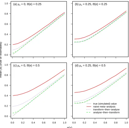
As suggested by theory, all three meta-analytic approaches yielded unbiased results of the 259
overall means, and are not considered further. Also as expected from analytical results (equation 260
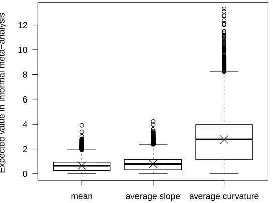
6), naive summary statistic-based meta-analysis of mean absolute values are upwardly biased, 261
across a range of parameters (figure 1). Simulation results support various features of the 262
analytical expression for bias (equation 6): the bias is greatest when sampling variance is high, 263
and especially when sampling variances are high relative to true variances. While the theoretical 264
analysis did not deal with situations where the true mean is non-zero2, the simulations give
265
2Expressions for bias in the mean absolute value when the mean is non-zero can be written down; however, I was unable to
fairly intuitive results. When the true mean is not zero, mean absolute values are less biased, 266
in informal meta-analyses. 267
For the range of parameters investigated, the standard ‘transform-then-analyse’ formal meta-268
analytic approach was consistently biased. The bias was intermediate between the naive meta-269
analysis and the ‘analyse-then-transform meta-analysis’. The bias in this formal approach to 270
meta-analysis arises because the model for sampling error in the random effects meta-analysis 271
is a poor reflection of the distribution of sampling errors of absolute values. The distribution of 272
sampling errors will be highly skewed for modest estimates with substantial uncertainty (i.e., 273
when σ(m)i is large relative to |xˆi|), while the mixed-effects meta-analysis assumes normal 274
errors. 275
The ‘analyse-then-transform’ approach, i.e., of modelling the raw meta-data, i.e., the ˆxi 276
values rather than the derived |xˆi| values, and then deriving the mean absolute value, was 277
unbiased across the majority of the range of parameter values. To some extent, this can be 278
interpreted as the analysis being a match to the data-generating mechanism. It is true that I 279
simulated the data under the statistical model that the mixed-effect meta-analysis applies to 280
values of ˆxi and their associated standard errors. However, this type of model might in fact 281
often be a very reasonable approximation to how values in many meta-datasets are obtained. 282
This meta-analytic approach was slightly upwardly biased at the very lowest values of the true 283
variance of x. This is because I constrained the estimate of σ(x) to be positive, and so at the 284
smallest true values of σ(x), the estimate must be at least a slight over-estimate (in general, it 285
is hard to imagine an estimator of a variance that is constrained to be positive, that will not 286
be upwardly biased for small true values). Since the absolute value depends positively on the 287
variance, this generates slight upward bias at the smallest true values. 288
Here, I have only focused on meta-analysis of the mean, and of the mean absolute values. 289
There are of course many other quantities that may be of interest in a meta-analysis. Most 290
quantities that are derived from quantities in the literature, according to a non-linear function, 291
will be biased in informal and ‘transform-then-analyse’ meta-analyses. In addition to the mean 292
(but not the mean absolute value), quantities such as regressions should generally be unbiased, 293
estimates of birds’ singing rates from different studies. Suppose that standard errors of singing 295
rates were not available. We have seen that the estimate of mean singing rate would not be 296
biased in a summary statistic-based informal meta-analysis. Similarly, we should not expect an 297
inference of the average regression of singing rate on a predictor variable, such as a measure of 298
forest cover, to be biased in informal meta-analyses. In contrast, quantities such as variances, 299
mean absolute values, or the mean absolute differences among treatments, all depend on the 300
dispersion of values among studies, and will therefore be biased in informal meta-analyses, and 301
will also be biased in ‘transform-then-analyse’ approaches to formal meta-analysis. 302
5
Re-analyses of informal meta-analyses
303
5.1 The average magnitude of natural selection
304
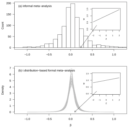
Kingsolver et al. (2001) reported on an informal meta-analysis of selection gradients and dif-305
ferentials (Endler, 1986; Lande, 1979; Lande and Arnold, 1983). One of their most important 306
findings is that non-trivial directional selection is common in nature. They report an average 307
magnitude of variance-standardised directional selection gradients of 0.23 (the full distribution 308
is depicted in figure 2a)3. As we have seen (equation 6), this finding potentially represents a
309
substantial over-estimate, due to sampling error. The average standard error of selection gradi-310
ent estimates in the database is about 0.15. So, in the improbable but instructive hypothetical 311
scenario where there was no selection in any study (just statistical noise arising from finite 312
sample size), the estimated mean absolute value of selection gradients that would be inferred 313
in an informal meta-analysis would be on the order of 314
r
2
π ·0.15 = 0.12.
Re-analysis 315
I used a mixed model to decompose the observed variation in selection gradients into that 316
arising from statistical noise and that which may represent real variation. The model took the 317
3There is a small difference in the mean absolute value of directional selection gradients in the database as a whole (0.23), and
form 318
ˆ
βi = ˆµβ +mi+ei. (10)
ˆ
βi are estimated selection gradients, and µ is the model intercept, or the estimated mean 319
selection gradient. miare measurement errors, which are of course unknown, although we know 320
they are drawn from estimate-specific distributions approximately following mi ∼ N(0, SEi2). 321
ei are residuals, and are assumed to follow ei ∼N(0,σˆ2(β)), where ˆσ2(β) is estimated. I then 322
derived an estimate of the mean absolute value of selection as the mean of a folded normal 323
distribution (equation 7) defined by the mixed-models estimates of ˆµβ and ˆσ2(β). To produce a 324
comparable mixed model-based analysis that does not account for sampling error, I also fitted 325
the model 326
ˆ
βi = ˆµβ +ei. (11)
I fitted both models using MCMCglmm (Hadfield, 2010), using default diffuse priors. I then
327
derived the mean absolute value of selection gradients as the expectation of a folded normal 328
distribution defined by the parameters estimated in the models defined by equations 10 and 329
11. 330
Accounting for statistical noise generates an estimate of the variance of selection gradients 331
of 0.0156 (i.e., from the model in equation 10; this is the posterior mode of the parameter in the 332
mixed model; this statistic is used for estimates throughout), with a 95% credible interval of 333
0.0121 - 0.0207. By contrast, the model in equation 11 yields a variance of estimated selection 334
gradients of 0.0775 (95% CI: 0.0689 - 0.0890). The corresponding standard deviations are 0.12 335
(95% CI: 0.11 - 0.14) and 0.28 (as for the estimate from the raw data, see above, with 95% CI: 336
0.26-0.30). 337
The model-based estimate of the average magnitude of selection gradients obtained as the 338
mean of a folded normal distribution is 0.10 (95% CI: 0.09 - 0.12). The corresponding estimate 339
based on the estimated selection gradients without accounting for sampling error is 0.23 (95% 340
CI: 0.21 - 0.24), which closely matches the estimate obtained by simply calculating the mean 341
of the absolute values of all the estimated directional selection gradients in the database. 342
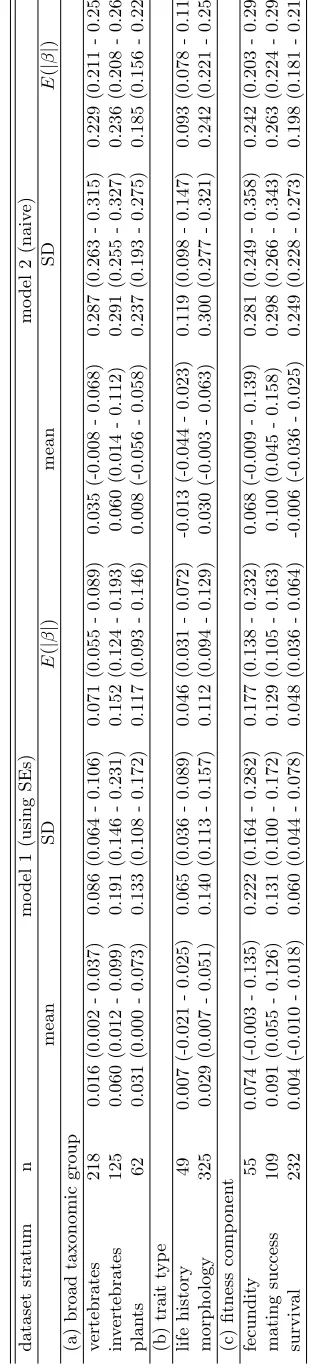
analysis of any given study, the average strengths of selection for different strata of the King-344
solver et al. (2001) dataset are clearly of interest. I therefore ran the basic mixed model 345
analyses, with and without accounting for sampling error, for several major subsets of the 346
database, continuing to focus on directional selection gradients. Because (a) analyses are (cor-347
rectly) much less apparently powerful when accounting for sampling error, and (b) sample sizes 348
for some strata are small and further reduced by incomplete reporting of the standard errors 349
necessary for meta-analysis, I did not conduct every possible analysis. Rather I subsetted the 350
database taxonomically for vertebrates, invertebrates, and plants, by trait type for life history 351
and morphology, and by fitness component for fecundity, mating success, and survival. 352
The general pattern that the magnitude of selection is inflated in analyses that do not 353
account for statistical noise at the level of individual estimates is supported at every level within 354
the database that I considered (table 1). Selection for life history traits is weakest, but this 355
probably reflects the definition used for life history traits. Many of the traits represent timing 356
in the life cycle, rather than life history traitssensu stricto, i.e., as in variables defined by a life 357
table. The general previously-reported patterns hold for means of selection gradients, which 358
are not expected to be biased by sampling error. Selection is generally positive for morphology, 359
and positive selection often acts through mating success (this may be primarily driven by 360
selection for morphology). Statistical noise at the level of the meta-analysis is increased (see 361
credible intervals reported in table 1), relative to the magnitudes of the estimates, in the formal 362
model that accounts for sampling error at the level of the component studies. This does not 363
represent a decrease in statistical power, but rather an improvement in realism relative to the 364
over-optimism of analyses that do not account for statistical noise. 365
The normal approximation to the distribution of selection gradients assumed in the residual 366
structure of a model such as that in equation 10 may generally provide a pragmatic and robust 367
approach to investigating components of variation in any observed dataset. However, we may be 368
interested in other aspects of the distribution. For example, it is very reasonable to think that 369
the true distribution of selection gradients may have thicker tails than the normal distribution. 370
I therefore constructed a model that is analogous to that in equation 10, except that the 371
This model takes exactly the same form as equation 10, except that the normal distribution 373
from which the ei are drawn is replaced by the three parameter t-distribution with mean zero 374
(because the model contains an intercept), and estimated variance and degrees of freedom. 375
The distribution of selection gradients from the t-distribution based model is depicted in 376
figure 2b. Comparison to figure 2a shows the dramatic difference between the distribution of 377
estimated selection gradients and the underlying distribution of selection gradients. The inset 378
figure depicts the relationship between unit variance-standardised trait values and relative 379
fitness that is implied by the average magnitude of estimated selection gradients, which is very 380
strong selection (see arguments in Hereford et al. 2004);|β|= 0.22 corresponds to approximately 381
a 2.5-fold change in fitness over a range from two standard deviations below to above the mean 382
phenotype. Such a selection gradient clearly does occur in nature (figure 2b), but is far rarer 383
than the original informal meta-analysis suggested. The mean absolute magnitude of directional 384
selection gradients in the t-distribution model4 is 0.090 (95% CI: 0.076 - 0.108). 385
Other inferences about the mean absolute value of selection 386
Knapczyk and Conner (2007) argued that the mean magnitude of selection gradients in King-387
solver et al.’s meta-analysis was not inflated by sampling error. Their analysis relied on sub-388
sampling from a restricted array of very large datasets. This is a potentially very useful ap-389
proach, but it relies on an assumption that the relevant properties of the restricted array of 390
datasets are the same as in the larger database. Close inspection reveals that this cannot be 391
the case in this instance. The restricted array of estimates ofβ in Knapczyk and Conner (2007) 392
contains some very large selection gradients including β = 1.12 for selection of flower number 393
via seed production, and three gradients of the fifteen in the Knapczyk and Conner (2007) 394
dataset have an absolute value above 0.5. 395
Inspection of the raw data from the Kingsolver et al. (2001) database (Kingsolver et al.’s fig-396
ure 5, figure 2a here), reveals that such large selection gradients are very far from representative 397
of the data as a whole. The selection gradients in Kingsolver et al. (2001) have larger sampling 398
errors, overall, than those in the Knapczyk and Conner (2007) dataset, and this larger sampling 399
4obtained asR
|x|d(x|µ, σ2, k)dx, whered(x|µ, σ2, k) is the density of the three parameter t-distribution with meanµ, variance
error can only inflate the apparent frequency of very large selection gradient estimates. If such 400
large (true) selection gradients were similarly frequent in the study systems from which the 401
Kingsolver et al. dataset was constructed, then similarly large (or larger) estimated selection 402
gradients would be similarly common, and they are not (Figure 2a). Furthermore, the few 403
selection gradient estimates of similar magnitude in the meta-database come exclusively from 404
studies with very small sample size (Kingsolver et al., 2001) - precisely those that would be 405
expected to yield estimates of large magnitude due to sampling error alone. 406
Note that Knapczyk and Conner (2007) made no errors that cause their dataset to be non-407
representative; it is simply by inspection of the distribution of estimates in the Kingsolver et al. 408
(2001) database that it is apparent that no true underlying distribution of selection gradients, 409
observed with sampling error, can be compatible with the high frequency of very large estimates 410
in the Knapczyk and Conner (2007) analysis. The similarity between the results of Conner et 411
al.’s analyses and the distribution of selection gradient estimates in the Kingsolver et al. (2001) 412
dataset is coincidental, and does not conflict with the inevitability that sampling error will 413
(potentially greatly) inflate estimates of the magnitude of effects in informal meta-analyses. 414
Hereford et al. (2004) clearly described the statistical mechanism by which sampling error 415
can inflate inferenes of the mean magnitude of selection. They applied a post-hoc correction for 416
sampling error using reported standard errors, and investigated the effect on the inference of the 417
mean absolute values of selection gradients. Their correction was not expected to completely 418
alleviate the problem, and the degree to which it solved the problem was not clear. Their 419
partially-corrected estimate of the mean absolute value of selection gradients was consequently 420
intermediate to that given by the original informal meta-analysis, and the formal model-based 421
analysis presented here. 422
Finally, Kingsolver et al. (2012) reported on an effort to apply a formal meta-analysis to 423
an updated database of selection gradient estimates. They performed several analyses of a 424
database originally presented in Kingsolver and Diamond (2011), which combined datasets 425
from Kingsolver et al. (2001) and Siepielski et al. (2009). Their position on the effects of 426
accounting for error is unclear. They specifically state, with respect to quantities such as 427
studies, and also that there are large effects of accounting for error (which previous studies did 429
not do). 430
Kingsolver et al. (2012)’s inference of the mean absolute value of selection, accounting for 431
sampling error, is much greater than their inference based on a naive analysis (which they 432
refer to as ‘uncorrected|β|’). This is a mathematical impossibility, or at least could only occur 433
if the properties of selection gradient estimates that are reported with and without standard 434
errors are vastly greater than seems plausible. It seems likely that some error occurred in 435
those analyses. My own re-analysis of the combined dataset reveals a mean absolute value 436
of estimated selection gradients (i.e., via informal meta-analysis) of about 0.21, both for the 437
subsets of the data with and without reported standard errors. This contrasts sharply with 438
the the ‘uncorrected’ value of about 0.05 reported in Kingsolver et al. (2012). I was able to 439
closely replicate their estimate of the mean |β| from formal mixed effects meta-analysis (the 440
analyse-then-transform approach) of about 0.14. 441
It may initially seem that the inference of the mean absolute value of selection from the 442
combined Kingsolver et al. (2001) and Siepielski et al. (2009) databases should be superior, as 443
it is based on a larger sample size. However, the credible intervals of the mean |β| from the 444
Kingsolver et al. (2001) and combined datasets do not overlap (95% CIs of 0.09 - 0.12 and 445
0.14 - 0.17, respectively). Therefore there must be some underlying difference between the two 446
databases. Specifically, in that portion of the estimates from the Siepielski et al. (2009) study, 447
which are temporally-replicated studies, must have stronger selection on average. I suspect that 448
people will be mostly inclined to invest long-term efforts in studies of traits that they already 449
know to be under selection. If this is the case, then the studies contributing to the original 450
Kingsolver et al. (2001) dataset might give the best impression of the average magnitude of 451
selection across a wide range of trait types and scenarios. 452
5.2 The frequency and magnitude of sexually antagonistic selection
453
Cox and Calsbeek (2009) present an informal meta-analysis of sexually antagonistic selection. 454
They report that 41% of pairs of selection coefficient estimates, obtained for each sex for 455
deviations of male and female selection coefficients (gradients and differentials combined) are 457
0.37 and 0.34, and the correlation between them is 0.19. The coefficient estimates are plotted 458
in figure 3a. The coefficient estimates that have associated standard errors are plotted in figure 459
3b. 460
The mean standard errors of selection coefficients are 0.17 for males and 0.20 for females. 461
The sex-specific sampling errors are expected to be uncorrelated, i.e., due to statistical noise 462
alone, there are few conditions in which studies that overestimate the true value of a selection 463
coefficient in one sex are no more or less likely to overestimate the corresponding coefficient 464
in the other sex. I simulated a set of random numbers, with one number corresponding to 465
every selection coefficient in the meta database that had a reported standard error. These 466
random numbers all had expectations of zero, and variances determined by the square of the 467
standard error. The distribution of these samples reflects the instructive though implausible 468
scenario of the distribution ofestimated sex-specific selection coefficients that would arise in the 469
hypothetical situation where no selection occurred in either sex in any study from the literature. 470
Thus, this scenario can give some insight into the influence of sampling error alone on inferences 471
of the frequency of sexually-antagonistic selection. The distribution of these hypothetical data 472
points is given in figure 3c; in this scenario, statistical noise causes approximately 50% of 473
estimates to appear to be sexually antagonistic. A key feature of the pattern in figure 3c is 474
that, no matter how many estimates are included in the informal meta-analysis, a substantial 475
impression of sexually-antagonistic selection will result, as a result of sampling error at the 476
level of the individual studies. 477
We can treat the problem more formally. Cox and Calsbeek (2009) used a measure of 478
sexually-antagonistic selection based on the absolute difference between paired male and female 479
selection coefficients 480
ˆ
SAi =|Sˆm−Sˆf| (12)
where ˆSm and ˆSf are estimated male and female variance-standardised selection coefficients 481
(either differentials or gradients). Cox and Calsbeek (2009) provide a discussion of how this 482
true distribution of selection coefficients in males and females is bivariate normal, and that 484
sampling errors of male and female selection gradients are both normal and uncorrelated, we 485
can derive an expression for the bias in an informal meta-analysis of sexually-antagonistic 486
selection. 487
The variance of the distribution of differences in true selection coefficients in males and 488
females is 489
σ2(Sm−Sf) =σ2(Sm) +σ2(Sf)−2σ(Sm, Sf) (13)
whereσ2(S
m), andσ2(Sf) are the variances in true selection coefficients in males and females, 490
and σ(Sm, Sf) is the covariance of true selection coefficients. The variance of the distribution 491
of differences in estimated selection coefficients in males and females is 492
σ2( ˆSm−Sˆf) = σ2( ˆSm) +σ2( ˆSf)−2σ( ˆSm,Sˆf)
=σ2(Sm) +σ2(m)Sm+σ
2(S
f) +σ2(m)Sf −2σ(Sm, Sf), (14)
whereσ2(m)
Sm andσ
2(m)
Sf are the sampling variances of male and female selection coefficients.
493
The mean absolute value of the difference between two independent draws from the same 494
normal distribution is 495
E[|xi−xj|] =
2
√
πσ(x) (15)
(Nair 1936, eq. 35). The bias in an informal meta-analysis of SA can therefore be written 496
using equations 13, 14 and 15 497
2
√ π
q
σ2(S
m) +σ2(m)Sm+σ
2(S
f) +σ2(m)Sf −2σ(Sm, Sf)−
2
√ π
q
σ2(S
m) +σ2(Sf)−2σ(Sm, Sf)
=√2 π
q
σ2(S
m) +σ2(m)Sm+σ2(Sf) +σ2(m)Sf −2σ(Sm, Sf)− q
σ2(S
m) +σ2(Sf)−2σ(Sm, Sf)
.
(16)
The expression is inelegant, but we can see that the quantity in brackets will be positive any 498
time that σ2(m)
Sm and/or σ
2(m)
Sf are positive, which in practice will always be the case.
Re-analysis 500
I constructed a bivariate-response mixed model to partition (co)variation in sex-specific pairs 501
of selection coefficients into portions arising from sampling error, and reflecting the underlying 502
biological pattern. The model took the form 503
Sm,i
Sf,i
=
µm
µf
+
mm,i
mf,i
+
em,i
ef,i
(17)
whereSm,iand Sf,iare the male and female-specific estimates for pairs of selection coefficients5 504
indexed by i. Sampling errors are assumed to be drawn according to 505
mm,i
mf,i
∼N
0
0
,
SE2
m,i 0
0 SEf,i2
and residuals according to 506
em,i
ef,i
∼N
0
0
,
σ2(m) σ(m, f)
σ(m, f) σ2(f)
where residual variances and covariance of male and female selection gradients, σ2(m), σ2(f),
507
and σ(m, f), as well as the sex-specific means in equation 17 are estimated parameters. I 508
implemented the model injags(Plummer, 2010), with diffuse normal priors on the sex-specific
509
means and a redundant prior parameterisation on the residual covariance matrix of selection 510
coefficients. 511
The mean selection coefficient in each sex is positive: males: 0.092 (95% CI: 0.040 - 0.153), 512
females: 0.074 (95% CI: 0.030 - 0.108). Critically, male and female selection coefficients covary 513
strongly and positively. The residual covariance matrix obtained by fitting the model described 514
5The analysis is conducted on a mix of selection differentials and gradients, following Cox and Calsbeek 2009. This combination
in equation 17 (95% CIs in brackets) is 515
σ2(m) = 0.067 (0.054−0.106) σ(m, f) = 0.038 (0.024−0.054)
r(m, f) = 0.794 (0.666−0.928) σ2(f) = 0.029 (0.016−0.045)
;
note that the sub-diagonal element is reported as the correlation. The consequence of this 516
positive correlation of male and female coefficients is that sexually antagonistic selection is 517
rare, and when it occurs, it is typically not highly antagonistic. Simulated values drawn form 518
the inferred joint distribution of male and female selection coefficients are plotted in figure 3d. 519
The proportion of pairs of selection coefficient estimates that differ in sign6 is 20% (95% CI: 12
520
- 25%). Furthermore, when selection is sexually antagonistic, it is also weakest. 521
Figure 4 shows the distributions of two possible metrics of sexually-antagonistic selection. 522
These metrics are calculated both from the raw data, i.e., by informal meta-analysis, and 523
calculated from the ‘analyse-then-transform’ analyses made possible by the bivariate response 524
random regression model. The first metric (figure 4a) is the distribution of products of male 525
and female selection coefficients. This quantity is negative when selection takes different signs 526
in the two sexes, and positive when selection is of the same sign. Values near zero indicate that 527
there is little selection in one or both sexes. The second metric (figure 4a) is Cox and Calsbeek 528
(2009)’s measure based on the absolute value of differences in male and female coefficients. 529
The model specified by equation 17 does not account for different levels of non-independence 530
in the data. Accounting for statistical non-independence is not expected (on average, i.e., the 531
analysis presented to this point is not expected to be biased) to change the inference about the 532
underlying variance and covariance of sex-specific selection coefficients. However, accounting 533
for non-independence may change our impression of how precisely we have characterised any 534
given overall effect. A source of non-independence considered by Cox and Calsbeek (2009) 535
is that pairwise reports of sex-specific selection coefficients from the same study tend to be 536
6obtained byR R Sm·Sf
|Sm|·|Sf|·N([Sm, Sf]
T, µ, σ)dS
mdSf, whereµandσare the mean vector and covariance matrix of selection
similar. I therefore fitted the model 537
Sm,ij
Sf,ij
=
µm
µf
+
mm,ij
mf,ij
+
rm,ij
rf,ij
+
em,ij
ef,ij
(18)
where r denotes study, and j indexes the studies to which individual records belong. As 538
above, the upper left elements are variances associated with male selection coefficients, the 539
bottom right correspond to female selection coefficients, and the entries above the diagonal 540
are covariances, and below the diagonal are correlations. The covariance matrix from which 541
the r values are assumed to come is constructed and estimated equivalently to the residual 542
covariance matrix (described above), and all other model components are treated as they were 543
for the model described by equation 17. 544
The between-study and within-study covariance matrices of paired sex-specific selection 545
coefficients are 546
"
0.034 (0.009−0.066) 0.021 (0.004−0.055) 0.996 (0.504−1.000) 0.025 (0.009−0.069
#
, and
"
0.041 (0.029−0.071) 0.015 (0.007−0.028) 0.678 (0.398−0.901) 0.012 (0.005−0.022)
#
,
respectively. The male variance is in the top left and the female variance is in the bottom right. 547
95% CIs are in brackets. The sub-diagonal element are the correlations. The total (co)variances 548
and correlations are thus 549
0.075 (0.049−0.119) 0.045 (0.021−0.075)
0.755 (0.496−0.905) 0.043 (0.021−0.084)
.
Accounting for non-independence among data points that come from the same studies therefore 550
does not appreciably change the overall pattern. The credible intervals of the total variance 551
components obtained from the second model are slightly larger and are probably more appro-552
priate. Differences in whether or not selection is sexually antagonistic or not seem to arise more 553
from differences among traits, than from differences among studies. 554
Sexual dimorphism and sexually antagonistic selection 555
Cox and Calsbeek (2009) considered whether any association exists between sexual dimorphism 556
between these phenomena might indicate that the evolution of sexual dimorphism generally 558
has resolved sexual conflict, while a positive relationship would indicate a general pattern of 559
ongoing conflict between the sexes. In the context of the analyses pursued to this point, a 560
relationship between sexual dimorphism and sexually antagonistic selection would primarily 561
be manifested as a (statistical) dependence between sexual dimorphism and the covariance 562
between male and female selection coefficients. Methods for estimating the dependence of a 563
covariance on a continuous variable are not well developed. 564
Standard modelling procedures do not exist to accommodate hypotheses about how covari-565
ance structures vary according to continuous variables. Therefore, determining how typical 566
magnitudes of sexually antagonistic selection covaries with a predictor such degree of sexual 567
dimorphism would deserve an independent study in itself. Here I make only a preliminary 568
attempt. A model structure that may be pragmatic would be to treat the correlation of male 569
and female selection gradients as a continuous function of the degree of sexual dimorphism, 570
and model the shape of that function as a sigmoidal relationship ranging between -1 and +1. 571
I therefore parameterised the correlation as 572
rSm,Sf,i =
2ea+b·Di
1 +ea+b·Di −1 (19)
where α and b are the regression parameters controlling the shape of the logistic curve that 573
is scaled between negative and positive one (note that 1+eae+ab+·Dib·Di would represent a logistic 574
curve between 0 and 1). rSm,Sf,i can then be thought of as the correlation that would be
575
observed among a group of paired sex-specific selection coefficients, all from systems with 576
sexual dimorphism Di. I used the absolute value of the measure of sexual dimorphism avail-577
able in the Cox and Calsbeek (2009) database, which is the difference between sex-specific 578
means. I specified the variances of the sex-specific selection coefficients independently, and 579
then obtained the dimorphism-dependent covariance of paired sex-specific selection coefficients 580
asrSm,Sf,i p
σ2(m)p
σ2(f).
581
The parameters of the regression of rSm,Sf,i on the degree of sexual dimorphism are α: 2.2
582
of b is greater than zero. Thus the overall pattern appears to be for sexual dimorphism to be 584
associated with a reduction in the degree of sexually antagonistic selection, although the value 585
of the coefficient controlling this pattern has a posterior distribution that substantially overlaps 586
zero. It is not surprising that this regression has a very large standard error. Considering that 587
each pair of estimates does not provide a concrete datapoint, but rather a very uncertain 588
inference about sexually-antagonistic selection, the formal meta-analysis may correctly have 589
great uncertainly in measures that seem easily estimable in an informal meta-analysis. The 590
correlation between male and female coefficients in the absence of sexual dimorphism is thus 591
about 0.85, while at higher levels of dimorphism, the correlation approaches one. 592
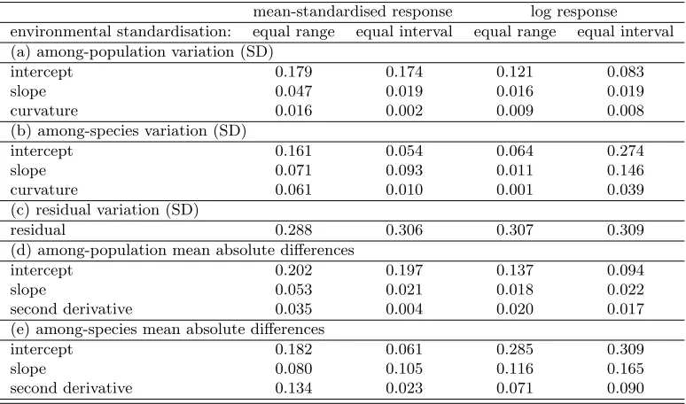
5.3 Population and species differences in reaction norm shape
593
Murren et al. (2014) report on differences between average values, slopes, curvatures, and 594
higher-order aspects of the shapes of reaction norms between species and populations. Their 595
primary conclusions include (1) that shapes, i.e., slopes and curvatures, of reaction norms 596
evolve more than average trait values, and (2) that curvature of reaction norms evolves more 597
than the slope. Statistical noise will inflate apparent differences between parameters such as 598
means7, slopes and intercepts. Furthermore, depending on the scaling of the environmental
599
variables, statistical noise will contribute differently to apparent variation in means, slopes and 600
curvatures. Therefore, sampling error alone will create specific patterns in the mean absolute 601
differences of averages, slopes, and curvatures of pairs of reaction norms. 602
A simple simulation may be instructive. Again, we will start with a simple situation with 603
trivial biology, and focus on how unbiased statistical noise in the literature may be converted 604
into superficially, and misleadingly, biologically interesting patterns in a naive meta-analysis. 605
Assume that some large number of studies are conducted, and that in each, two populations 606
are assayed for mean phenotype in each of three (ordered) environments. Assume that every 607
7Here, four different words will be used for aspects of the average value of a reaction norm. The mean will represent the population
population in every study and in every environment has the same mean value (the mean value 608
is actually irrelevant), and that the standard error of the mean is 1 unit in every case (this 609
value is also completely irrelevant to the pattern that results, so long as it is non-zero). For 610
this null scenario, I simulated data, and calculated the difference in means between populations 611
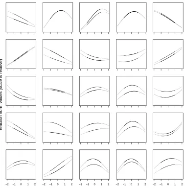
(species) for each of the simulated studies, as well as the differences in slopes and curvatures, 612
following the expressions used by Murren et al. (2014). The distribution of the magnitudes, 613
i.e., absolute values, of these differences is plotted in figure 5. Murren et al. (2014) report 614
estimates of mean absolute differences in reaction norm components from an analysis that is 615
weighted by (the square root of) sample size. Note that weighting does not solve the problem 616
illustrated here. A well-designed weighting scheme will be analogous to the transform-then-617
analyse approach to meta-analysis, which can perform poorly for arbitrary derived quantities 618
(figure 1). Consider that these simulations assume equal error across all estimates, which may 619
occur if (among other things) there are equal sample sizes. As such, weighting by sample size 620
would provide a trivially identical result to an unweighted analysis, and the spurious pattern 621
would remain. 622
The pattern in figure 5 can also be obtained analytically. Again, I will focus on the scenario 623
where there are three environmental treatments, as these dominate the available data. Assume, 624
as above, that a pair of reaction norms (e.g., a congeneric or conspecific pair) are identical. Let 625
the mean phenotypes in the three environments for one population be denoted ˆx1, ˆx2, and ˆx3,
626
and denote the corresponding three estimated mean phenotypes in the other population with 627
ˆ
y1, ˆy2, and ˆy3. Assume that all mean values are estimated with the same precision, such that
628
ˆ
xi ∼N(µ, σ(m)), ˆyi ∼N(µ, σ(m)). 629
The variance of the mean of the ˆx or ˆy values is 630
σ2(¯xˆ) =σ2(¯yˆ) = 3
1 3
2
σ2(m) = 1
3σ
2(m) (20)
which is simply the variance of three independent random values, each with the same variance. 631
The average of the slopes of the two line segments in each reaction norm is 12(ˆx2−xˆ1) +12(ˆx3−
632
ˆ
x2) = 12xˆ3−12xˆ1 (or equivalent expressions with ˆy). Therefore the sampling variance of average
slopes is 634
σ2(ˆxi−xˆi−1) = 2
1 2
2
σ2(m) = 1
2σ
2(m). (21)
Curvature (defined by Murren et al. 2014 as the difference of slopes between adjacent intervals) 635
for a study with three points is 636
(ˆx3−x2ˆ )−(ˆx2−x1ˆ ) = ˆx3−2ˆx2 + ˆx1
and so the variance in curvatures is 637
σ2((ˆxi+1−xˆi)−(ˆxi−xˆi−1)) = 2σ2(m) + 22σ2(m) = 6σ2(m). (22)
The mean difference between different reaction norm components is given by the expression 638
2
√
πσ, just as we used for the mean difference in male and female selection coefficients. Conse-639
quently, in the absence of any differences in reaction norms between conspecific or congeneric 640
populations, a pattern in estimated mean differences in means, slopes, and curvatures will arise 641
by sampling error alone. In our toy model, the pattern will be: 642
2
√ π
r
1 3σ
2(m)
for means 643
2
√ π
r
1 2σ
2(m)
for slopes, and 644
2
√ π
p
6σ2(m)
for curvatures. This pattern will be super-imposed on any true differences among these prop-645
erties of reaction norms in nature. 646
Re-analysis 647
Distributions of intercepts, slopes, and curvatures can be modelled using mixed effects models, 648
based estimates of differences in properties of reaction norms, I fitted the model 650
xijk =A+B·Ej +C·Ej2
+ar,k+br,k·Ei+cr,k·Ei2
+as,j+bs,j·Ei+cs,j·Ei2
+ap,i+bp,i·Ei+cp,i·Ei2
+ei.
(23)
This is a quadraticrandom regression mixed model. xijk are the environment-specific estimated 651
mean values, and Ei are the corresponding values of the environmental covariate (expressed 652
as treatment intervals in the raw data). I standardised the environment-specific estimated 653
means in two ways. Murren et al. (2014) divided by the overall mean, and I did this as well. 654
Furthermore (and see discussion below) a scaling that may better facilitate inference of both 655
intraspecific and congeneric variation in reaction norms is to log (actually ln(x+ 1), as there 656
are zero values in the data) transform, and so I used logged data as well. i indexes studies, and 657
j indexes paired estimates within studies. A, B, and C are the average intercept, slope, and 658
curvature. The a, b, and c terms are the study-specific (or rather trait within study) random 659
intercept, slope and curvature terms, associated with study r, species s, and population p. I 660
modelled these terms as being drawn from the multivariate normal distribution 661
a
b
c
x,y
∼N
0
0
0
,
σ2(a) σ(a, b) σ(a, c)
σ(a, b) σ2(b) σ(b, c)
σ(a, c) σ(b, c) σ2(c)
y
where the parameters of the covariance matrix ofai,bi, andci values are estimated parameters, 662
with x ∈ {k, j, i} and y ∈ {r, s, p}. I modelled the residuals as coming from a common 663
distribution, i.e., eij ∼N(0, σ2(e)). 664
I have preferred Bayesian approaches for all analyses (except simulations) to this point. 665
While the random regression mixed model of variation in reaction norms can be fitted in a 666
variance components. This is not surprising (with hindsight), because only studies with four or 668
more environmental treatments can contribute to inferences about intercepts, slopes curvatures, 669
and residual variance. To avoid the need to use essentially arbitrary priors, I fitted this model 670
by restricted maximum likelihood, usinglme4(Bates et al., 2014). Standard errors for variance 671
components in random regression models are not easily obtained from this software, and in 672
any case can be misleading when variance components are small and imprecisely estimated. I 673
therefore report only the (restricted) maximum likelihood estimates of the parameters of the 674
simplest model that reports parameters that are analogous to the main quantities reported by 675
Murren et al. (2014). These should be interpreted in the light that, given the model and the 676
currently-available data, the inferences about curvature are highly uncertain. 677
The scaling of the environmental variable, E in equation 23, is important to consider. Mur-678
ren et al. (2014)’s calculations of means, slopes, and curvatures assume that all intervals be-679
tween environmental treatments have equal meaning. This is one of two potential treatments. 680
Assuming equal biological meaning of all intervals assumes that those studies that use fewer 681
environmental treatments cover a proportionately smaller portion of the relevant range of the 682
environmental variable. I think that an alternative treatment may be more sensible. It seems to 683
me more likely that, on average, most studies are designed to span most of the relevant range of 684
environmental conditions, whatever that range may be for the study, species, populations, en-685
vironmental variable, and traits in question. If this second option represents a more reasonable 686
model of how reaction norm studies are generally designed, the consequences of assuming equal 687
scaling of intervals, rather than equal scaling of the total environmental range, may be serious. 688
If two studies covered the same range of the environment, the one with fewer increments of 689
environmental conditions within that range would have greater calculated slopes and curva-690
tures than the study with more increments, and thus would also have relatively exaggerated 691
differences between slopes and curvatures if equal scaling of increments was assumed. 692
Because neither treatment of the environmental variables is an obviously superior approach 693
for every study in the database, I applied both standardisations. These can be seen as useful 694
extremes, with truths for how each study was designed typically lying somewhere in between. 695