Tracking of wireless devices: is it possible and solvable?

(1)

Master’s thesis

Tracking of wireless devices:

Is it possible and solvable?

Remie Löwik July, 2018

Supervisors:

Dr.ir. P.T. de Boer Prof.dr.ir. G.J. Heijenk Dr. M. Baratchi

(2)

Abstract

A shared research experiment is performed to prove that tracking of Wi-Fi enabled clients is possible. Then individually a solution for the problem is developed, verified and tested. In this case the goal was to alter the protocol in such a way that tracking was not possible any more but to keep interoperability with older devices.

In the shared experiment students are asked to track their household occupancy and devices that collect Wi-Fi data are placed in student households for a week. Using the collected Wi-Fi data an occupancy schedule is generated and compared to the actual schedule created by the student. Unfortunately the schedule could not be generated because the students were all on the same network (Eduroam) which made it impossible to separate households and their devices from their neighbours.

(3)

Figures

Figure 1: Confidence level vs sample size for the university campus household list ... 7

Figure 2: Measurement equipment ... 9

Figure 3: Example of a timesheet day before and after initial processing ... 11

Figure 4: Signal strength distribution of the measured devices in 1 household ... 17

Figure 5: Detected presence of two visually matched devices against the user’s schedule ... 19

Figure 6: Dataset 1, comparison between network traces and user's schedule ... 21

Figure 7: Dataset 1, comparison between the user's schedule and measured absences ... 21

Figure 8: Dataset 2, comparison between network traces and the user's schedule ... 22

Figure 10: Dataset 3, comparison between the user's schedule and measured absences ... 23

Figure 15: Average false and correct vacancy prediction rate versus device count ... 26

Figure 16: Average false and correct vacancy prediction rate versus device count #1 ... 27

Figure 19: Example timesheet ... 29

Figure 20: privacy preserving discovery (Lindqvist et al. 2009, figure 1) ... 35

Figure 21: Probability of tracking devices (Vanhoef et al. 2016, figure 6) ... 35

Figure 22: SlyFi Protocol (Greenstein et al. 2008, figure 1) ... 36

Figure 23: Generic MAC frame header ... 41

Figure 24: Frame control field ... 41

Figure 25: Ack only sequence of frames ... 45

Figure 26: Acknowledgement frame ... 45

Figure 27: Clear to self sequence of frames ... 45

Figure 28: Clear to Send frame ... 45

Figure 29: Request to send sequence of frames ... 46

Figure 30: Request to Send frame ... 46

Figure 31: Beacon sequence of frames ... 46

Figure 32: Beacon frame ... 47

Figure 33: Beacon frame body ... 47

Figure 34: Probe sequence of frames ... 47

Figure 35: Probe request frame ... 47

Figure 36: Probe request frame body... 47

Figure 37: Probe response frame ... 48

Figure 38: Probe response frame body ... 48

Figure 39: Open authentication sequence of frames ... 48

Figure 40: Shared key authentication sequence of frames ... 48

Figure 41: Authentication frame ... 49

Figure 42: Authentication frame body ... 49

Figure 43: Association sequence of frames ... 49

Figure 44: Association request frame ... 50

Figure 45: Association request frame body ... 50

Figure 46: Re-association request frame ... 50

(6)

2

Figure 48: Association response frame ... 51

Figure 49: Association response frame body... 51

Figure 50: Disassociation frame ... 51

Figure 51: Disassociation frame body... 51

Figure 52: EAP key exchange sequence of frames... 52

Figure 53: EAP frame ... 53

Figure 54: EAP frame header ... 53

Figure 55: EAP-Key frame ... 53

Figure 56: EAP-Key frame body ... 53

Figure 57: Key information field ... 54

Figure 58: Data transmission sequence of frames... 54

Figure 59: CCMP frame format ... 55

Figure 60: CCMP header ... 55

Figure 61: PS-Poll sequence of frames ... 55

Figure 62: Power-save Poll frame ... 55

Figure 63: Comparison between key sizes (Ajay Kumar et al. 2013, table 4) ... 56

Figure 64: Performance comparison between RSA en ECDH (Levi and Savas 2003, figure A) ... 57

Figure 65: Used data structures ... 60

Figure 66: Adding MACs to the encrypted MAC list ... 60

Figure 67: Updating encrypted MAC list... 61

Figure 68: Location of changes ... 62

Figure 69: Beacon transmission handling ... 63

Figure 70: Beacon receive handling ... 63

Figure 71: Probe and authentication transmission handling ... 64

Figure 72:Probe and authentication receive handling... 64

Figure 73: PS-Poll/Other transmission handling ... 65

Figure 74: Data/Other packet receive handling ... 65

Figure 75: Overview of execution path ... 77

Figure 76: Overview of the setup ... 78

Figure 77: Beacon data structure ... 79

Figure 78: Connection data structure ... 79

Figure 79: Kernel Wi-Fi stack ... 81

Figure 80: Wireshark trace of authentication... 81

Tables

Table 1: User presence results with their respective standard deviations ... 19

Table 2: Overview of comparison ... 37

Table 3: Overview with new solution ... 38

(7)

3

Abbreviations

ACK Acknowledgement

AES Advanced encryption standard

AID Association id

ATIM Announcement traffic indication map windows BSSID Basic service set identifier

CBC Cipher block chaining

CCMP Counter mode cipher block chaining message authentication code protocol

CFB Cipher feedback

CTR Counter mode

CTS Clear to send

EAPOW Extensible authentication protocol over wireless ECB Electronic codebook

ECDH Elliptic curve Diffie-Hellman FCS Frame check sequence KCK Key confirmation key KEK Key encryption key MAC Media access control MIC Message integrity code MiTM Man in the middle

NAV Network allocation vector

OFB Output feedback

PSK Pre shared key

PTK Pairwise transient key RC4 Rivest cipher 4

RTS Request to send

SSID Service set identifier TIM Traffic indication map

TK Temporal key

(8)

4

1 Introduction

In a world where the digital world becomes ever more important, the devices we use to access that world also changes. In 2007 less than a third of the users were mobile users (“Mobile marketing statistics 2018,” 2018), but after 2014 this already grew to more than half of the users and still continued to grow afterwards. What all these mobile devices have in common is the methods of how they communicate, the most common methods are mobile connections like 3G and 4G and Wi-Fi. Although users are more privacy-aware nowadays, little is known by those common users about how much information is leaked by especially the latter of the communication methods.

(9)

5

2 Shared research

2.1 Introduction

This chapter covers the research into trackability of household occupancy using the Wi-Fi network. This research is a follow-up of an earlier small-scale research (see appendix 1) performed by the same researchers among the households of relatives. The usability of that research was very limited due to the scale and potential bias. This research tries to prove the potential of Wi-Fi eavesdropping to track occupancy in households.

The execution of this research is a joint effort between Remie Löwik, Ruben Lubben and Tim Kers. These researchers performed their own research into potential solutions against Wi-Fi tracking. This chapter, assessing the potential risk of eavesdropping on Wi-Fi networks is a joint effort between Remie and Tim and will be identical between their respective theses.

The research is divided into 2 parts. Due to practical reasons, the measurements are conducted in the living quarters on the campus of the University of Twente. These living quarters feature a shared Wi-Fi network called Eduroam. Instead of separating the devices per household by their used network, as would be possible in normal households, this shared network throws all devices on one pile. Or at least from the burglar’s perspective.

The first research step, would be to use other parameters to determine the critical devices for the participating household. After this step, the situation is again similar to normal households where only relevant devices are registered. At this point, the trackability of the network can be determined. This chapter therefore knows two research questions:

 Is it possible to determine which Wi-Fi devices belong to a certain household in a shared network with only passively detectable parameters?

(10)

6

2.2 Background

As stated in the introduction, this research was preceded by a small-scale experiment in 2016. In this small-scale research, borrowed laptops were used as measurement devices which limited the group of participants to relatives and friends. Unfortunately, the stability of the borrowed hardware and the many configurations onto which the software had to work proved to be a problem. Combining this with a very limited timeframe, limited the experiment to 12 households. This in turn limited the statistical relevance of the research.

The results, however, did indicate a potential problem with household Wi-Fi networks. On average, 86.7% of predictions were correct. The 13.3% faulty predictions were made up of false occupied (10.5%) and false vacant predictions (2.8%). For a burglar, false occupied predictions are potentially missed opportunities. However, as long as other opportunities are available, this is not really a problem. The false vacant predictions are problematic for a burglar. These are the times they would think the house was vacant while it was not and would risk getting caught.

Most of these false vacant predictions occurred at night, partly due to households having limited Wi-Fi coverage in the bedrooms causing residents to turn their Wi-Fi off at night. When the 00:00 to 07:00 timeslot was removed from the analysis, correct ratings increased to 89.3%, false occupied declined to 10% and false vacant diminished to 0.7%.

Although less relevant to this research, a small social study was conducted as well. It showed that participants felt slightly less safe in their neighbourhood, with safety grade lowering from 7.5 before and 7.33 after the research, on a scale of 10. More people had the feeling of being unsafe in their homes (50% before to 58.33% after) and the likeliness of a burglary happening to them in the next 12 months was graded 1.6% higher than the 25% before the research.

The social part of the previous research was not included in the new research. This was mainly due to the amount of time and effort it involved to get all participants to fill in the forms. The forms also required more work from participants, which was deemed as a potential deal breaker for them. Additionally, this research focuses on the technical side of this potential problem. The social study is not regarded as relevant for this part.

(11)

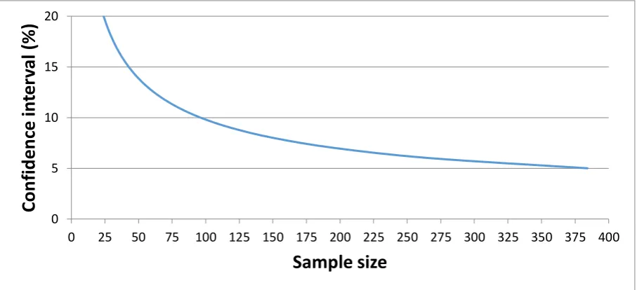
7 In statistical experiments the required number of samples can be determined by (Lisa Sullivan, PhD, n.d.):

𝑛 = (𝑍𝜎 𝐸)

2

[image:11.595.72.526.199.406.2]

Where, Z is dependent on the confidence level. In this case, 95% yields a Z of 1.96. 𝜎 Indicates the standard deviation, which is fairly unknown at this point and therefore set to 50%. E is the margin of error which is plotted against the sample size (n) in Figure 1 below

Figure 1: Confidence level vs sample size for the university campus household list

To reach sub-10% intervals, sample sizes of 100 and higher are required, which is not feasible with our pool of participants. Therefore, a compromise was made to aim for a 15% or better confidence interval and the accompanying requirement of 43 or more datasets. This was deemed feasible with the available time and equipment and keeping in mind some problems on the way.

0 5 10 15 20

0 25 50 75 100 125 150 175 200 225 250 275 300 325 350 375 400

Co

n

fi

d

e

n

ce

in

te

rv

al

(

%)

(12)

8

2.3 Method

This experiment is split into three parts. First, measurement equipment is placed in the homes of participants to gather network traces to be used in the later parts. The residents receive a form on which they are asked to keep their presence to be compared with the retrieved data afterwards. After retrieval, the filled-in timesheet and trace data are pre-processed to prepare for the next parts. In the second part, the pre-processed data is processed to remove any device not belonging to that household.

The third part would then aim at extracting an occupancy schedule from the network trace and compare this to the schedule filled in by the participant.

2.3.1 Part 1: gathering network traces from households

In the original experiment, datasets of multiple weeks were recorded to try and recognize recurring patterns in people’s lives. In this research, the datasets are chosen to be only one week long, to try and reach a higher number of datasets in the available time frame for this research. The focus therefore lies on reliable occupancy detection instead of pattern recognition. When occupancy detection can be performed reliably, pattern detection should not be a problem.

As the research potentially involved privacy sensitive data of the occupants, the research proposal was reviewed by the Ethical board of the EEMCS faculty at the University of Twente. This gave some restrictions on target groups and data storage that will be explained further down in this chapter. 2.3.1.1 Target group

A problem with the earlier experiment was the use of relatives as test subjects, this gave potentially biased data and therefore should be avoided in the new experiment. For this new experiment, subjects should be chosen at random from a large pool of potential candidates.

The ethical board gave an important restriction on the potential candidates. All occupants in a participating household must be able to understand and consent to the potential privacy risk. This prohibits measuring households with for example underage children or mentally challenged people. Eventually the aim was set on student housing. This gives an easily containable set of candidates, almost no underage people and very small chances of children living in and/or visiting the household. This left two possible groups: Dormitories and individual living quarters. Dormitories posed a couple of potential problems.

 When measuring a complete dormitory, all students living there must consent. With living groups up to 16 people, it is not unlikely that at least one would refuse.

 Standard measurement equipment would probably lack the range to cover the complete dormitory, thus requiring more equipment and opening the door for synchronisation issues and/or potential blind spots.

Alternatively, measurements could focus on individual occupants in a dormitory. A measurement device could then be placed in the room of the participating student. However, this gives a similar range problem. When a student leaves his room to eat in the shared living room, he or she is likely to be out of range. This system would consider this as “absent”. The student should therefore note his presence in the actual room, which quickly becomes a hassle and error prone.

(13)

9 2.3.1.2 Privacy considerations

As this research involves privacy sensitive information about people and their household, some precautions had to be taken:

 No user data is stored by the measurement device at all

 The device identifier (the MAC address) is only stored as a hash to stop anyone from finding easily finding the original device. Although scanning the whole campus could still be easily done, preventing such action is fairly hard whilst keeping usable data.Additionally, anyone with such interest would be better suited with gathering newer data instead of trying to crack the old.

 The retrieved timetable is linked to the measurement device its device number. However, this number is never linked to a house address, phone number or email address. This means that there is no way to link a dataset or timetable back to a household or individual.

 After retrieving the measurement device, all data is removed from the SD-card before reusing it for another household. Although the stored data would be barely usable for any adversary, this prevents other people from retrieving the data.

 All research data is to be permanently removed no later than 1 year after completing the research, as stated in the original research proposal (see appendix 1). The data is only accessible to the researchers and supervisors stated in the proposal and brochure.

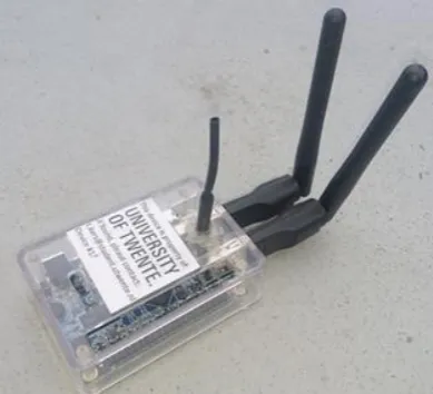
2.3.1.3 Measurement equipment

For these measurements a device was required to capture network traffic. As student housing is covered with the Eduroam Wi-Fi network, monitoring this network is sufficient in most cases. The network is divided over the three Wi-Fi super channels (channel 1, 6 and 11) thus requiring 3 network interfaces. The choice fell on the Orange pi lite minicomputer. This creditcard sized

computer features an onboard Wi-Fi module (XR819) and two additional USB ports for two additional USB Wi-Fi card (Ralink RT5370).

An important parameter was the support for monitoring mode on the Wi-Fi interface. This was a problem with selecting a Raspberry pi. Its on-board module does not support monitoring mode requiring us to add 3 external Wi-Fi modules. Furthermore, the cost of a raspberry pi is almost double that of the Orange pi Lite.

[image:13.595.71.266.563.740.2]

For the OS (Ubuntu) and measurement data, a 16GB micro SD card is used. With data compression used in our system, this would easily cover measurement data for multiple weeks.

(14)

10 2.3.1.4 Data gathering

When the device is started, it places all three Wi-Fi modules in monitoring mode. In this mode, the module will listen to all traffic on that frequency regardless of destination or network. In this case the modules will be set up to listen all three super channels. By using monitor mode, the module does not have to be associated with any network to listen to the data that is transferred on that channel. The traffic is monitored for each interface separately by creating a TCPdump instance for each of the interfaces. TCPDump was configured to return only the data we required, in this case the following information was stored to file for each packet:

 Source device  Destination device  Timestamp  Signal strength  Packet type

The output of TCPDump was then parsed by a java program and then processed further for storage. Due to privacy concerns, instead of storing the MAC addresses of the source and destination device, an anonymized hash is created and stored. Furthermore, user data in the packet is not stored. It would not be relevant for the research and take a lot of storage space, but it is also a privacy concern.

Each interface writes its data to a set files. Then after an hour, a new set of files is started and the old files are flushed and closed to make sure that all packets are committed to storage. This technique also helps in preventing data loss. If a device loses power suddenly, depending on the current activity of the system, data could be lost. By storing the data in chunks, this data loss is limited to a maximum of 1 hour.

Furthermore, the choice was made to split up the information into three different files: data-, mac- and extra packets file. The first file is the data file. In this file the mac addresses, a timestamp, signal strength and packet type is saved for each packet that is received on the interface and is directly compressed with the GZIP compression algorithm to minimize the size of the data. Because mac addresses are the biggest portion of the data, the choice was made not to rely on the compression algorithm but instead to make a lookup table in which all the MAC addresses are given an ID. This ID is then used in the data file instead of the longer MAC address.

The second file is the content of the lookup table: an ID with its assigned MAC address. But before saving the mac addresses, the macs will first be hashed using the SHA256 hash function. In the end this lookup table did not only save storage space but also minimized the chances of errors: Hashing and storing the MAC addresses only once minimizes the change for errors. Furthermore, extra processing is saved by only having to hash each MAC address once instead of having to hash the macs for each received packet.

(15)

11 2.3.1.5 Measurement procedure

From the original list of households, a random selection of 60 households at a time is chosen by a Matlab script using the standard rand() function with a random seed of 42. These households receive an introductory letter about the research to give them some time to consider participating. Then, after approximately a week, the houses are visited and the residents asked if they would like to participate in the research. If required, additional information can be given. If nobody is home at that time or the participant wishes some extra time to consider participating, the household is tried again at a later time. Obviously, a resident is free to decline participation without reasoning, after which the house is removed from the list.

When a resident chooses to participate, one of the measurement devices is handed over and plugged into a power socket inside the house. Additionally, the subjects get a form with a timetable on which they are asked to keep their presence log during the measurements. This timetable is used as a reference to validate the conclusions drawn from the measurement data. For extra information about the research, the privacy concerns and proper actions, should they want to stop the

measurements, an informational brochure is handed over for them to keep. Finally, the participant is asked for contact information such as a phone number or email address so that, after a week of measuring, the participant can be contacted for retrieval of the device and timetable.

The introductory letter, blank timesheet and informational brochure are added in appendix I of this report.

2.3.1.6 Initial data processing

After retrieval of the measurement device and timetable, their data has to be processed before it can be used to identify occupancy.

Timesheet processing

All timesheets are scanned and digitally processed. Initially, the “marked” fields are made uniformly black to prevent reading error by the automated processor. An example of this is shown in Figure 3.

Figure 3: Example of a timesheet day before and after initial processing

After this step, the images are loaded into an automated processor, created in Matlab. This program lines up the filled in timesheet with a reference (empty) version and determines the light level of each data field (white or black, indicating unmarked or marked). For this, predetermined coordinates are used, derived from the reference timesheet.

Participants were allowed to choose if they preferred to mark for “absent” or “present” as long as they indicated their choice on the timesheet. Additionally, participants sometimes mixed up days or started marking at a different day than the first one on the form. All these factors were manually entered into the processor, which (where applicable) inverted the derived schedule or rearranged the days.

(16)

12

Trace data processing

As discussed in saving data part, the device saves three files per interface per hour. The choice was made to do some pre-processing on this data to lower the amount of data that had to be processed every time. To do this a program was written that would read and uncompress this data and summarize the presence for each device. This was done by creating blocks of 5 minutes in which packet type count, the minimum, maximum, average signal strength and to whom each client was talking to was saved. This data was then exported to a csv file to allow further processing in Matlab.

2.3.2 Part 2: Automated filtering of relevant devices

2.3.2.1 Selecting devices within the household

In a normal household environment, a burglar can select a certain network and therefore household to track. This allows him to only track devices using that network. Unfortunately, just as many universities, the University of Twente uses the Eduroam network across the entire campus including the living quarters. As a lot of students will be using this, the distinction between houses disappears. This means that other steps have to be taken to extract devices belonging to the targeted household. If this step succeeds, the remaining trace only contains legitimate devices for that household and the situation is again similar to a normal household.

Two factors were used to determine devices belonging to that household. The measurement device logged the signal-to-noise ratio of every received device throughout the week. With the device placed within the household, the devices with the highest ratings will most likely belong to that household.

(17)

13 2.3.2.2 Selecting devices with usable characteristics

Nowadays, many different devices can be present in networks. A burglar will probably be best served with smartphone availability, as this device is mostly carried around with the residents. Laptops, tablets and other devices could give similar information.

But a stationary device like a network printer, being active all day long, would not be very interesting to determine occupancy. Therefore, some extra filters are added to separate usable devices from the trace.

 Discard devices with high active or inactive rates

 A device that is communicating continuously or barely does not give much insight in any resident’s schedule. Therefore, any device that is active for more than 95% of the time or less than 5% of the time is discarded. The likelihood of a resident having such a schedule is almost zero.

 Session lengths

 Schedules differ between people, but some factors are fairly constant. Over the period of a week, one can expect the residents to be home for some lengths. For example, because they sleep at home. Therefore, a filter is created that looks at the occurrence of certain session lengths. For example, if a device is never present for a couple of hours, it is very unlikely that its trace will represent the residents schedule

 Session counts

 Similar to session lengths, session counts can be used as a parameter as well. A real person would not come home and leave every 10 minutes (for example), nor would they stay at home for 5 days and then disappear for the weekend. In the first situation, it is more likely that it involves a device connecting periodically. In the latter, it looks more like a stationary device, but it is turned off when the resident leaves for the weekend. Although exact

boundaries for “legitimate” devices are hard to draw, the extreme situations as stated above can be removed relatively safe.

2.3.3 Part 3: Extract household occupancy from network trace data

In a normal household, the Wi-Fi network would be used by the people and devices belonging to it. This makes tracking much easier as the trace would not be influenced by neighbouring devices. In the chosen Eduroam environment, all households share the same network. But after extracting the appropriate device traces from the dataset, the situation should again be comparable to a normal household.

The next step is to generate occupancy schedules from the network trace and compare this to the schedules filled in by the participants. A burglar will aim to minimize risk. As he will need only one free moment, it is less relevant if other potential moments go unnoticed due to an overly safe technique.

The safest options to start with is to regard every captured device as relevant. Only when all devices become silent, the house is regarded empty. In addition to that, a burglar would not be interested in free windows of a couple of minutes. Instead, only continuous vacancies of 15 minutes or more are deemed relevant.

(18)

14

2.4 Results

2.4.1 Part 1: gathering network traces from households

Gathering the network traces from the households proved to be a very time-consuming process. Apart from all the hours distributing introductory letters, asking for participation and retrieving devices, a lot of time was consumed by software issues on the measurement devices and to process the data.

2.4.1.1 Start-up phase:

Before being able to distribute any device, software had to be created for the measurement equipment. In this step, multiple test rounds were conducted to test the software for functionality and reliability. Some problems were found and resolved in this phase, like occasional failure to initialize a network interface. In these cases, one of the interfaces became unusable for the data logging software. As this problem was detectable and re-initialization of the module was sufficient, this problem was effectively resolved.

2.4.1.2 First measurement round:

After multiple rounds of short and long tests, the system was deemed ready for deployment. Unfortunately, after the first round of real-world tests, the resulting data from all 10 participating households came back corrupted. The cause of this was found to lie within the LZMA compression algorithm used to compress the recorded data.

The problem turned out to be a memory allocation issue and finding a solution within the

compression software proved difficult. Fortunately, storage space turned out to be plenty for a week of data allowing a switch to the more commonly used but less efficient Gzip compression algorithm. This solution was tested in multiple networks for multiple days and proved reliable.

2.4.1.3 Final measurement rounds:

After the problem in the first round of measurement was resolved, multiple successful measurement rounds were performed before the holidays put a stop to this research step. In total, 45 households participated in these rounds before the holidays brought a stop to them.

Of these 45, 8 were lost due to administrative mistakes. 6 of them were found to be checked off, but never actually retrieved. Due to the long period between data gathering and processing, this

discrepancy went unnoticed. The participants were contacted when this problem was found. The device was successfully retrieved from two residents. one admitted the device was never retrieved, but lost it while moving to a new house. The other three never responded.

Two other devices remain unaccounted for. It could be that they are also still out there with participants, but we were not able to find out whom. The strict separation between consent forms (with personal information) and devices and their data may be good for privacy concerns, but did prevent us from backtracking which consent forms were never met with data.

(19)

15 Although the major issues were resolved, some measurements still developed problems. Some of the found problems were:

 Measurement devices missing data from one of the network interfaces. This looks similar to the earlier initialization error, except that the software never found an initialization error nor were there any problems reported in the system’s logs. Normally, a problem with one of the network interfaces should trigger a system reboot to try to re-initialize everything. However, this did not happen and the system continued its operation with two interfaces. This problem only occurred in one of the measurements making a not completely plugged in USB Wi-Fi modules plausible.

 Measurement devices seized to record any data during the measurement period. Although the device was placed for a minimum of 7 days, the trace would only cover a couple of hours or days in some cases. Similar to the previous problem, no evidence of it was to be found in the systems logs. A possible cause could be a loss of power. Maybe a resident moved the device causing the power jack to become loose or unplugged an extension cord while forgetting the device that was placed there. In total, 5 devices showed these kinds of problems with their active time varying between 26 and 95 hours. One of these devices had its data split with a reboot in between. As the device does not have a real time clock, there is no data on the amount of downtime between these two sessions.

 Measurement devices developing corrupted files within the data. This could have been caused by a power loss or other reboot event. This problem affected two devices, but only influenced a couple of files. The software was created to store data in one-hour blocks to prevent large data loss in such cases. Therefore, the datasets remained usable, although missing an hour somewhere.

(20)

16

2.4.2 Part 2: Automated filtering of relevant devices

Due to the choice of an area with a single large Wi-Fi network, it was expected that neighbouring devices would be picked up in the measurement. The first step would be to remove these from the trace. The resulting dataset should ideally only include all devices belonging to the participating household. This situation would be similar to a measurement in a normal household where devices are separated by their used network.

2.4.2.1 Original approach

While processing the data, the number of unique devices recorded in the measurements proved to be extremely high. As the experiment was conducted in the Eduroam environment, it was expected that large amounts of devices would be found from neighbouring households. However, it was not expected that most datasets would contain hundreds of recorded devices and some which even went up to hundreds of thousands.

One cause for this huge number of devices is people passing by the house. This would result in a registration of their device (if active on Wi-Fi) for a short amount of time. Additionally, the MAC randomization scheme of some versions of IOS and Android would create a lot of “fake” devices as long as the devices has its Wi-Fi capabilities enabled but is not connected to a network.

Multiple rounds of filtering were used to try and remove any unwanted device from the traces. Initially, 5 datasets were picked as training set to adjust the filters. These filters would then be applied to the other datasets.

Remove extremely short and long presences

People walking by or devices with MAC randomization create a lot of data that is not usable for occupancy tracking. Therefore, all devices that were picked up for a total of less than 5% of the total measurement duration, or approximately 8 hours out of the week, were removed from the trace. This includes MAC randomizing devices, people walking by and someone visiting during the week. Additionally, devices that were present for more than 95% of the time were also removed. These devices include access points and stationary devices. These devices yield no information about the resident’s presence and are therefore fairly useless for a burglar.

This filter removed a major part of “unusable” devices from the trace and reduced the datasets mostly to sizes between 25 and 75 devices.

Group devices together by mutual communication

The idea behind this filter was that devices belonging to the same household are more likely to communicate with each other. For example, video streaming from a laptop to a TV, or sending a document to a network printer.

(21)

17

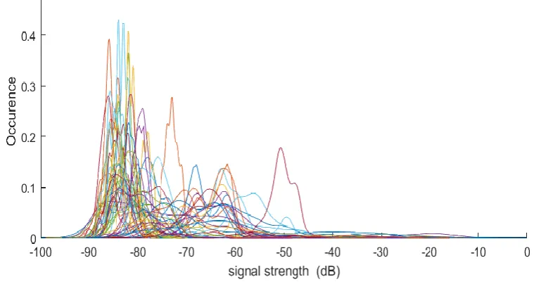
Remove devices with low signal strength

[image:21.595.100.480.255.457.2]

Devices within the household are in close proximity of the measurement device and should therefore read high SNR values. Finding the exact threshold after which a device does not belong to that house is going to be difficult due to all the different circumstances in and around the households. However, it can be used to filter out “distant” devices and reduce the dataset by a significant amount.

Figure 4 shows the signal strength distributions in one of the datasets gathered in this experiment. Most devices reside in the far left of the graph, making them most likely to be distant. However, it is difficult to select proper thresholds to distinguish devices actually belonging to the household. Manually comparing the dataset to the filled-in schedule revealed 1 perfectly matching device. However, when looking at the average signal strengths, that device came second with the first device showing no relation to the schedule. When looking at peak values, the matched device fell down to 16th place.

Figure 4: Signal strength distribution of the measured devices in 1 household

No similarity in the results was found across the datasets. The original training set of 4 datasets was even doubled to 8, to try and find the best matching filter settings. However, the filter was not able to remove all “unwanted” devices without losing genuine ones as well.

Another problem that arose, was the lack of “matching” devices in a lot of datasets. Although some devices showed high signal strengths, they would not be comparable to the schedule that the resident filled in. This problem is further worked out in 2.4.3: Alternative approach.

Session lengths

Analysis of the datasets showed some interesting characteristics in some devices. For example, some devices would show enormous amounts of activity, but all in short bursts.

Although it is unclear what kind of devices these actually are, but it is not likely to reflect the

schedule of a resident. An actual resident would normally have periods of presence and absence. To try and filter for those characteristics, session lengths were checked. It would be likely that a resident would have multiple presences of a couple of hours during the week, for example to sleep, study or relax.

(22)

18

Session counts

This filter had a similar aim to the previous one. During a week, a resident would probably leave a number of times. But to the rapid transitioning devices mentioned earlier showed extremely high numbers. Other stationary devices that had 1 period of absence would pass through the <95% filter, but would show very low session counts.

This filter was set out to filter out unrealistic low and high session count numbers. Although

reasonably effective, it did not have any influence over the session length filter. Therefore, this filter was eventually dropped.

2.4.2.2 End result

In the end, a uniformly applicable filter was not achieved. The filters, when combined, gave a

reasonable decline in device count, but returned both genuine and neighbouring devices. Even within the test group, with prior knowledge of the schedules, no acceptable result was achieved.

As mentioned earlier, many datasets appeared to be lacking “genuine” devices at all, when

(23)

19

2.4.3 Alternative approach

As mentioned before, a lot of datasets appeared to be lacking any devices matching to the schedule. This raised the question if occupancy tracking was even possible with the devices picked up by the measurement devices.

Therefore, instead of using a training set, all datasets were manually compared to the schedules to find any (seemingly) matching devices. Although time-consuming, the easiest method proved to be to plot (a subset of) the devices together with the schedule and visually match them together. Automated versions were tried, but they would occasionally miss devices or incorrectly match them. Sorting the devices by their mean signal strength proved to be effective. The matching devices would (as expected) usually occur in the top part of the selection. In the end, potentially matching devices were identified in only14 of the remaining 25datasets. In most households one of the identified devices would closely match a device. Any other would have a lot of resemblance, but also errors. Figure 5 shows a comparison between two visually matched devices and the accompanying schematic.

Figure 5: Detected presence of two visually matched devices against the user’s schedule

Both devices behave similar to the schedule. However, the bottom device often becomes

intermittent when the user is supposed to be away. This is likely to be the behaviour of a stationary device periodically checking the return of known devices. The real “user” schedule appears to be the middle graph.

To get an impression of reliability between the schedule and trace data, the visually best matching device of each household was selected and scored. These devices are likely to be smartphones and similar devices, closely representing the user’s presence. These results are presented in Table 1: User presence results with their respective standard deviations

below.

Correct occupied prediction Correct vacant predictions Total correct predictions

90,4 % ± 8,9% 87,6% ± 11,9% 87,8% ± 9,8%

Table 1: User presence results with their respective standard deviations

(24)

20

2.4.4 Part 3: Extract household occupancy from network trace data

As explained in part 2, the automatic filtering of devices proved problematic. The proposed method of only selecting relevant devices with filters and extract occupancy out of that is therefore difficult. Instead, this part is split into 2 parts. First, all visually matched devices of the household are

combined and scored. These devices are the most likely to reside within the same household. This combined dataset is compared against the user’s schedule to see if usable data has remained. Additionally, some of the filters of part 2 are reused. Although the filters were not able to remove all “wrong” devices, they may still be usable. If genuine devices are present in the dataset, combining them with “wrong” devices only removes potential vacant moments. But it does not add false vacant readings.

Unfortunately, this technique is only applicable to the datasets in which at least one device was recognized. As the measuring equipment lacked any means of measuring date and time, there is no way of lining up the measurements with the schedule without visual checks. A rough estimate can be made, but the manually checked datasets showed various amount of offset remaining.

2.4.4.1 Combining visually matched devices

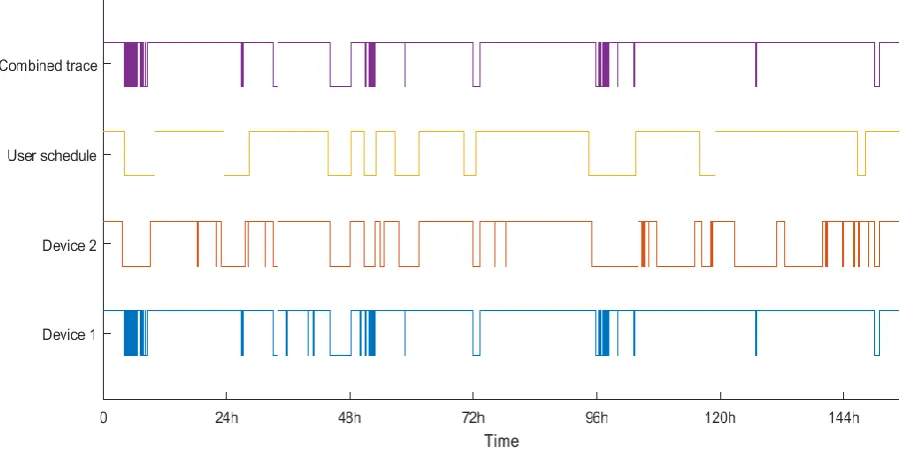
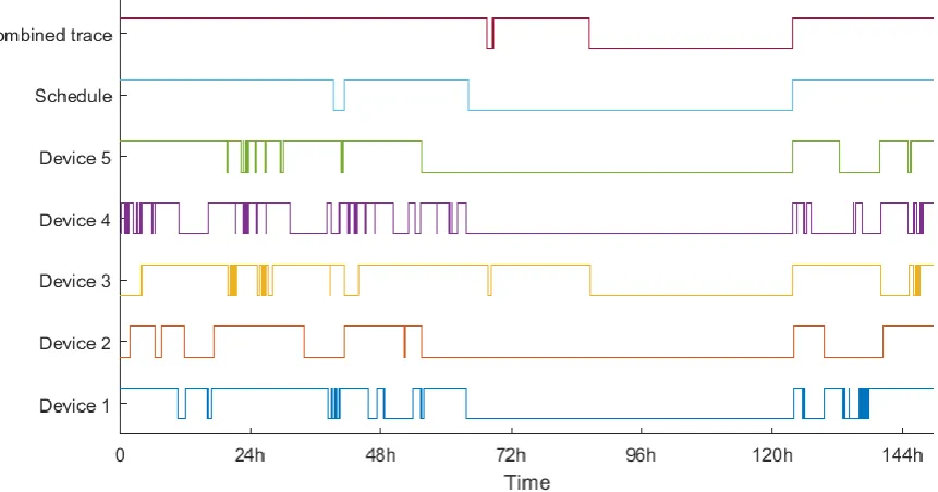
This technique was only applicable to 7 of 14 the households with visually matched devices. In the other 7, only one device was matched to the schedule. The single device matches were already covered in part 2. The remaining datasets had two (4 times), three (twice) or five (once) devices matched to their schedules.

For each dataset, the traces of all devices are combined into one. Combining the devices effectively performed an “OR” operation on the traces. If any of the devices is present at that moment, the combined trace is too. From a burglar’s point of view, this is the safest option. Only when no device is active, the house is regarded empty. The combined trace is added to the first figure presented for each dataset, this to give an overview of the used data.

(25)

21 2.4.4.2 Dataset 1

[image:25.595.76.528.168.393.2]

In the first dataset, 2 devices were recognized. Figure 6 shows their behaviour compared to the schedule. The 2 devices share a number of absences which in turn match roughly with the schedule. However, there is a slight offset between the absences in the schedule and the devices at some times. This could be down to small errors when filling in the schedule.

Figure 6: Dataset 1, comparison between network traces and user's schedule

As a burglar would not be looking for absences of mere minutes, some additional filtering was required. Figure 7 shows the original schedule and the combined trace, filtered for absences of more than 15, 30 and 60 minutes.

[image:25.595.81.518.476.727.2]

(26)

22 At this point, it is a bit problematic to decide which offset between measurements and schedules can be regarded as still valid. For example, the absence at 72 hours is measured slightly later than the schedule states, but there is a reasonable overlap. Completely at the right of the graph, the measured absence is shifted free of the schedule. They are reasonably similar in length and a schedule error is not unlikely, but there is no definitive answer. At the other hand, the measured absence at approximately 33 hours is shifted a lot more from the long-scheduled absence starting at 24h. Additionally, the duration is completely different as well.

These uncertainties make it impossible to capture the result in numbers, but they do give an impression. In this dataset, the longest measured absence (just before the 48h mark) matches perfectly with the schedule. Should the burglar’s measurements have returned this data, picking the longest absence would have been “safe”.

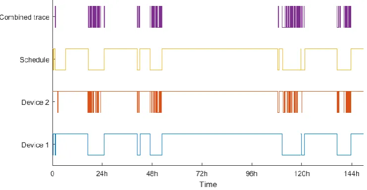
2.4.4.3 Dataset 2

The second dataset yielded 5 potentially matching devices although none of them prove to be a perfect match. The schedule did not give much room for comparison as it only showed two absences. It is not unlikely that the resident forgot to register some (maybe shorter) absences.

[image:26.595.80.511.374.600.2]

However, Figure 8 shows that combining these devices still give useful information. The long absence from the schedule largely returns in the combined trace. The smaller absence in the combined trace also matches with the large vacant slot of the schedule, giving this prediction an almost perfect score.

Figure 8: Dataset 2, comparison between network traces and the user's schedule

(27)

23 2.4.4.4 Dataset 3

Dataset 1 showed some “unstable” presence like a stationary device could create. In that dataset, it did not prove to be a large problem. This dataset however, has a device that influences the combined trace a lot.

[image:27.595.72.443.167.359.2]

Figure 9 shows the two devices recognized for this trace. One of which displays periodic activity when de resident is away from home.

[image:27.595.93.502.437.639.2]

When filtering this combined trace for periods of 15, 30 and 60 minutes, only a couple of options remain with a maximum length of just over an hour. Meanwhile, the schedule shows plenty of opportunities.

Figure 10: Dataset 3, comparison between the user's schedule and measured absences

(28)

24 2.4.4.5 Dataset 4

Also, with 3 recognized devices, dataset 4 also shows some “unstable” behaviour, especially in device 1. However, the influence is a lot smaller. Figure 11 shows that the large absences are still

[image:28.595.72.469.140.336.2]

recognized, although the largest absence is divided in multiple pieces.

Filtering with 15, 30 and 60 minute thresholds barely influences the combined trace apart from removing some of the fast switching. However, a burglar would have already chosen the large absence.

2.4.4.6 Dataset 5

In this dataset, two devices were found to be matching the schedule. However strangely, both traces were virtually identical to each other and the schedule. The combined trace of Figure 12 therefore needs no further filtering. The data already matches the schedule without any mistakes.

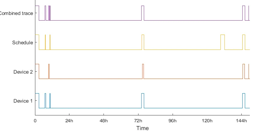
[image:28.595.73.518.474.661.2]

(29)

25 2.4.4.7 Dataset 6

[image:29.595.74.485.168.378.2]

Similar to dataset 5, both devices in this dataset are similar to the schedule. The combined trace therefore matches very well. However, Figure 13 shows the potential risk of using this kind of presence tracking. The schedule states that the resident was home at approximately the 130-hour mark, but both devices were silent. This would be a risk, should the burglar decide to abuse that “absence”.

2.4.4.8 Dataset 7

The last dataset had 3 matching devices as shown in Figure 14.

[image:29.595.74.475.426.652.2]

(30)

26 2.4.4.9 Combining top SNR devices

The usability of the previous results is severely limited. It only shows that device data could be used to determine occupancy. But to be able to do that, a burglar still has to extract the right devices from the full dataset without the prior knowledge of the schedule. When operating in a normal house network, the network itself will only be used by residents and maybe visitors removing this problem. Unfortunately, reliably extracting the appropriate devices from the large Eduroam dataset has proved impossible. This prevents us from proving that these techniques are reliable.

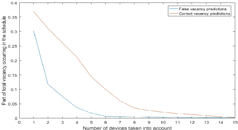
However, some use may still be present in the dataset. As stated earlier, a burglar is only interested in one opportunity, as long as it is reliable. Maybe, the filters were not perfect, but still good enough. To test this, the dataset is initially sorted by signal strength. Afterwards, the first device is taken and compared to the schedule, then the first 2 devices are taken together and compared and so on. The manually recognized devices mostly resided in the top part of the dataset when sorted by signal strength.

[image:30.595.101.519.338.566.2]

All these combinations produce a certain relation between the correct and false vacancy predictions. This relation, with the imperfections of “wrong” devices, may still be able to deliver usable data for a burglar. Figure 15 shows these combinations and their average false vacant and correct vacant scores as a part of the total vacancy displayed by the schedule.

Figure 15: Average false and correct vacancy prediction rate versus device count

The graph clearly shows that the false vacant occurrences decline as the number of devices increase, but so do the correct vacant occurrences. Instead of getting a sweet spot where the false vacant predictions become negligible and true vacant predictions still occur often, both factors follow reasonably similar declines.

The relative sweet spot seems to lie at 6 devices, but only 10% of the actual vacancies is still measured. And of those vacancies, 6% is false. Note that this graph shows an average across the 14 datasets with manually recognized devices. In a lot of household, the burglar will run a lot more risk as the spread between these are very large. Figure 16, 18 and 19 show three widely different examples of these datasets.

(31)

27 Figure 16: Average false and correct vacancy prediction rate versus device count #1

Figure 17: Average false and correct vacancy prediction rate versus device count #2

Figure 18: Average false and correct vacancy prediction rate versus device count #3

Unfortunately, the filters introduced in part 2 are not very helpful here either. The session count and session length filters require significant difference between “good” and “bad” devices, but almost all devices in the top segment of the list (with high signal strength) display a reasonable pattern for a person.

(32)

28

2.5 Problems and solutions

During the research, several issues arose with different consequences.

2.5.1 Limited effective time for data gathering

Initially, creating and testing the measurement equipment’s software took more time than expected. Afterwards, the first measurement round unveiled some unknown issues making this measurement round useless. Combined with the time limit of the upcoming summer holiday, at which most residents would be away from home for prolonged periods of time, limited the amount of

measurements that could be performed. Due to limited available time for the research project and all the other work that needed to be performed, continuation after the summer holiday was not a viable option.

To achieve larger amounts of datasets, a larger timespan would have been needed. More equipment would not have made such a difference in the current setting as on most occasions, not all

equipment would be distributed at the same time. The distributions of letters, visiting the residents and collecting of the gathered data required large amounts of time. Improving this part, especially the visits, would free a lot of time.

A potential option would be to increase the size of the household lists substantially. In the current experiment, random selections of 60 households were made. After a substantial amount of these were tried (and participated or declined), another 60 were added. These household would be

scattered all around the campus’ living quarters, which takes a lot of time to cover. Increasing this list drastically or maybe even dropping the randomized part (although this may interfere with the

defendability of the research) increases the number of households in every building and therefore saves a lot of “travel time” between them. This approach may require extra measurement

equipment for extra effectiveness as this large set of households will yield more participants in a single round.

(33)

29

2.5.2 The shared Wi-Fi network (Eduroam)

All buildings on the University’s campus are fitted with wireless access points distributing the

Eduroam network. This induced the problem that devices are no longer linked to a specific household as they would be in most normal households. This issue was known beforehand, but was expected to be countered by using SNR readings and other factors to determine “in-house” equipment.

Unfortunately, this proved to be problematic. In the households where devices were recognized manually with the resident’s schematic, the devices would rank very high in this classification. But in a lot of households, the difference between them and some other devices was marginal. Other devices would also frequently be classed higher than a device actually belonging to that household. With these datasets, that meant that reliable filtering of “correct” devices was impossible without the prior knowledge of the resident’s schematics.

Another issue was the apparent lack of matching devices in a large number of datasets. Although exact reasons are unclear, part of it seems to be connected to the limited coverage of the Eduroam network. Some participants stated that the Eduroam network in their living quarters was very weak and unreliable. This resulted in residents disabling their Wi-Fi functionality on their devices and reverting to the cellular network. Other residents created a personal Wi-Fi network in their homes. As long as this network would reside on one of the three super channels, also used by the Eduroam network, the measurement device would still be able to trace the network. But if another channel was used, they would fall outside of our measured frequencies and remain invisible.

There is also a possibility of residents using the wired network for devices like their computer. However, this is also an expectable factor in normal households.

2.5.3 Reliability of timesheets

The gathered network data was to be compared to the timesheet filled in by the occupant. However, there is no real way to determine the reliability of the schedule. In the datasets where devices were manually recognized, the timesheet was obviously comparable to the gathered data. But in the other datasets, this is an unknown factor.

Some timesheets show a very unusual schedule. This does not definitively say, that the sheet was filled-in incorrectly, but it does give that impression. Most notably is the timesheet of which one day is shown in Figure 19 below:

(34)

30 The rest of the timesheet shows similar absences of only 15 or 30 minutes, a couple of times a day. Although there is no definitive way of determining if this timesheet is correct, the strange schedule and the fact that no matching devices were present do give an impression that the schedule is not correct.

Without the shared Wi-Fi network, a burglar would not have to find matching devices out of a list. If the devices would represent this schedule, it would be quickly apparent that there are not really any usable timeslots in which the house is vacant. It is most likely that the burglar would skip this

household in favour of an “easier” one.

2.5.4 Absence of RTC

As already mentioned earlier in the report, the chosen measurement devices lacked a way of keeping time while unpowered. So, every time a device was placed, it would start measuring at the first of January at 0:00. Although this does not influence the measurements themselves, it does remove any synchronisation possibility with the schedule. A rough start time of the measurement may be known, but there is a lot of possibility for offset to occur. This was also seen in the datasets with visually matched devices. Data was shifted manually in relation to the given schedule, but the amount of shifting varied a lot.

(35)

31

2.6 Conclusion

This research was intended as a follow-up on a similar experiment. Instead of a small-scale experiment among (potentially biased) relatives, this research would be able to prove the risk of presence detection by Wi-Fi eavesdropping with enough statistical relevance.

The main question for this was similar to that earlier experiment.

 Is it possible to reliably track occupancy in a household with passive eavesdropping on its Wi-Fi traffic?

The experiment originally yielded 55 participating households where a minimum of 43 was set. Due to soft- and hardware problems, an administrative error and incorrectly filled in or missing forms the resulting number of datasets stuck at only 25.

Apart from the lower-than anticipated number of usable datasets, the research question proved impossible to answer in this experiment. This was mainly due to the chosen circumstances. Because of ethical considerations, households with underage or mentally challenged people were off limits. Therefore, student housing was chosen which gave the added complexity of a shared Wi-Fi network as compared to per-household networks.

This gave a second research question to be answered:

 Is it possible to determine which Wi-Fi devices belong to a certain household in a shared network with only passively detectable parameters?

Unfortunately, this proved to be difficult. The filters created to separate the devices belonging to the household from the rest were only partially effective at best. They reduced the number of devices, but optimal settings varied between households and “external” devices often remained in the dataset. Stricter settings resulted in correct devices being filtered out. Looking at communication between devices in the same household did not help either. It turned out that intercommunication happened everywhere in the network, regardless of the devices belong to the same household or not.

Eventually, manual selection of devices matching the schedule was performed as a last resort to get some usable data. Of the 25 remaining datasets, similarly behaving devices were only found in 14 of the datasets. Retuning the filters with this knowledge still did not return any usable filter settings. Matching devices usually showed high SNR figures as expected, but there often would be others too. This made predictions without prior knowledge completely unreliable.

Comparing the matched devices to their accompanying schedule does show that Wi-Fi data can represent actual occupancy. The predictions from the Wi-Fi data showed a match rate with the schedule of 87,80 percent. Unfortunately, this was only possible with visually matched devices using prior knowledge of the user’s schedule.

(36)

32

2.7 Discussion

The main goal of this research was to prove that occupancy detection from a household’s Wi-Fi traffic was possible. Unfortunately, this question proved impossible to tackle with the chosen circumstances. This was mainly caused by the shared Eduroam network in the chosen student living quarters. A normal household would have its own private network, making all devices on it relevant for the burglar. In the chosen situation, it proved impossible to reliably separate devices from each other based on their household. This prevented any proper research into the main goal.

Visually matching devices did show that network traces can show occupancy, but these results are not really defendable as it only covered a small amount of household and required prior knowledge. To allow for better results, a number of potential improvements have been thought of on the way. The first and most straightforward one would be to stop using the shared network environment and revert to normal households. The reason this was not done in this experiment was a limitation posted by the ethical board preventing us to use houses with underage or mentally challenged people. In normal neighbourhoods, this omits a large number of houses making the experiment a lot more cumbersome.

However, the given limitation is, from our point of view, not really necessary. The main reason for this restriction would be that these people would not be able to understand the privacy risk that they are exposed of. However, again in our opinion, there is no realistic risk in this. The data stored is not linked to any house or person. It also does not say anything about the timeframe in which the experiment was conducted. Should someone obtain the data and somehow find out which house it belonged to and who carries which device in that house, it would still be old data of unknown age. If someone is going through so many lengths to obtain data, they are better of gathering it themselves. When looking at the experiment as it was conducted, a couple of other improvements should be put in place.

To improve the efficiency of deploying the devices, larger groups of people should be contacted at the same time. In this case, a group of 60 households was chosen at a time. After a reasonable part of that participated or declined, an extra 60 households were added. As these households were randomly scattered around the campus, it took a large amount of time to visit them all. Instead, adding more households to the “active” list makes the rounds more efficient. Some research has to be done into the maximum possible list size while preventing a bias in the list.

Additionally, a passage could be added to the introductory letter to ask people to contact us when they would like to participate. This would not replace going to all the housed, but could give an initial list of participants to go to. The sooner a device is set out, the sooner it is back and can be set out again. As the number of devices is limited, this addition could aid in a more efficient use of the equipment.

(37)

33 Another option would be to add a form of communication to the device. In this experiment, Wi-Fi would be the most obvious. Initially, the devices had such functionality. When booted, they would set up a management network to connect to. This allowed some checking of functionality.

Unfortunately, this system introduced more reliability problems after which it was disabled. This system was also limited to the initial boot. A better system would be continuous or periodic communication options. This would allow for periodic checks, preventing small errors to ruin

complete datasets. However, this functionality would require an extra network adapter or a periodic downtime on one of the channels while the communication path is opened temporarily.

(38)

34

3

3.1 Introduction

There are already many implementations, which reduce the trackability of Wi-Fi enabled devices. In this chapter these implementations are divided into different categories. The implementations are then shortly explained: how they work and their similarity with other solutions. After which a comparison is made between the different categories. This comparison is then used to define the goal of this research.

3.2 Awareness

The first category is not about solving the trackability problem but simply about improving the awareness of the trackability/privacy problems.

The paper “PriFi beacons” (Könings et al., 2013) is not actually a solution to the trackability problem but more a solution that improves the awareness of the problem. This is done by adding information about privacy implementations onto beacons transmitted by the access point. They then

implemented an application, in android, which reads this information and shows it to the users. This is not an actual solution to the problem but is still important because it tries to improve the

awareness of privacy problems with the current protocol.

3.3 Passive probe

The second category is called passive probe, this is because it involves probe requests/responses and it does not actually change the protocol in any way (that is why it is passive in a sense). This is mostly done by randomizing the sender mac address and removing SSIDs from the probe request.

The paper “How talkative is your mobile device?”(Freudiger, 2015) tries to quantify how many probe requests an average smartphone shares with the world. It also researches how effective the

implementation of mac randomization is by testing the implementation of an Iphone with IOS 8, which includes these features. Their results show that mobile phones send on average about 55 probe requests per hour. This part of the research shows mainly that the current implementation of the Wi-Fi protocol makes tracking of phones very easy. Furthermore, the effectiveness of the randomizing the mac addresses is shown to be very ineffective in its current implementation. The first problem with its implementation is that it only works while the devices are asleep, it does not randomize its mac while awake. The second problem is that it does not change other fields in the header that could be used to link packets together.

3.4 Active probe

The third category is called active probe because changes are made to the protocol to the probe requests and responses to decrease the trackability and improve privacy.

(39)

35 The paper “Privacy-preserving 802.11

access-point discovery” (Lindqvist et al., 2009) is about changes in the 802.11 protocol to preserve privacy in access point discovery. The proposed changes are minimally enough that interoperability with the 802.11 protocol is kept. Currently a client transmits a probe request to which an access point can respond with a probe response. After which authentication and association requests are transmitted back and forth to complete the connection. The problem with these packets is that

identifiable data is sent in all these packets.

This paper solves this by removing the identifiable data from the probe packets and uses randomized MAC address for the association and authentication packets (as shown in Figure 20).

3.5 Passive mac

The fourth category improves on the probe categories as it actually improves multiple parts of the 802.11 standard that leak information about the device. This again is done without changing the protocol. In the paper “Enhancing location privacy in wireless LAN through disposable interface identifiers” (Gruteser and Grunwald, 2005), they try to reduce trackability by using disposable MAC addresses and renewing these addresses regularly.

In this implementation, they periodically generate a new MAC address after which they reconnect to their network if they were connected. This solution does have some drawbacks, since a new connection is made every time the address is changed; no active connections are possible while changing identifiers.

The paper “802.11 user fingerprinting” show that mac randomization does not work alone as other identifiers in the MAC header make it possible to still track a device (like packet size)

As does the paper “Why MAC Address

Randomization is not Enough “(Vanhoef et al., 2016) show that using random mac addresses are not enough to prevent the client from

being tracked, as shown in Figure 21 the probability of a device being tracked is above 50% with 16 devices connected. This is due to other information that is leaked by the client. Furthermore, they show that they could get the real mac address using two methods that are described in the paper.

Figure 20: privacy preserving discovery (Lindqvist et al. 2009, figure 1)

Tracking of wireless devices: is it possible and solvable?

Master’s thesis