An orientation field approach to modelling fibre generated spatial point processes

(1)

University of Warwick institutional repository: http://go.warwick.ac.uk/wrap

A Thesis Submitted for the Degree of PhD at the University of Warwick

http://go.warwick.ac.uk/wrap/49422

This thesis is made available online and is protected by original copyright.

Please scroll down to view the document itself.

(2)

An Orientation Field Approach to Modelling

Fibre-Generated Spatial Point Processes

by

Bryony J. Hill

Thesis

Submitted to the University of Warwick

for the degree of

Doctor of Philosophy

Department of Statistics

(3)

List of Tables

5.1 Summary of moves in birth-death MCMC . . . 73

6.1 Results for first simulated example . . . 109

6.2 Results for simulated example from Stanford and Raftery, 2000 . . . 112

6.3 Results for earthquake data . . . 115

6.4 Results for fingerprint pore data . . . 118

6.5 Results for simulated helix data . . . 122

6.6 Results for galaxy data . . . 125

(8)

List of Figures

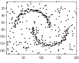
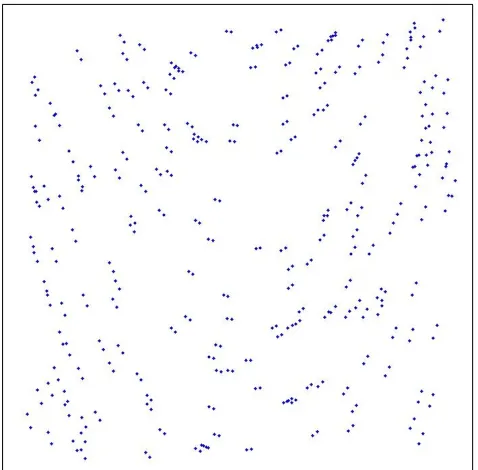
1.1 Four examples of point patterns clustered around curvilinear features 2

2.1 A simulated example of a Glass pattern using an exponential

rans-formation . . . 7

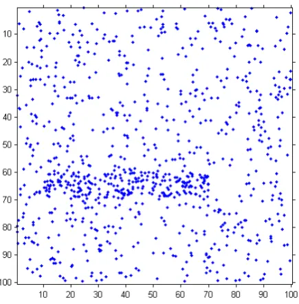
2.2 A simulated example of minefield data . . . 14

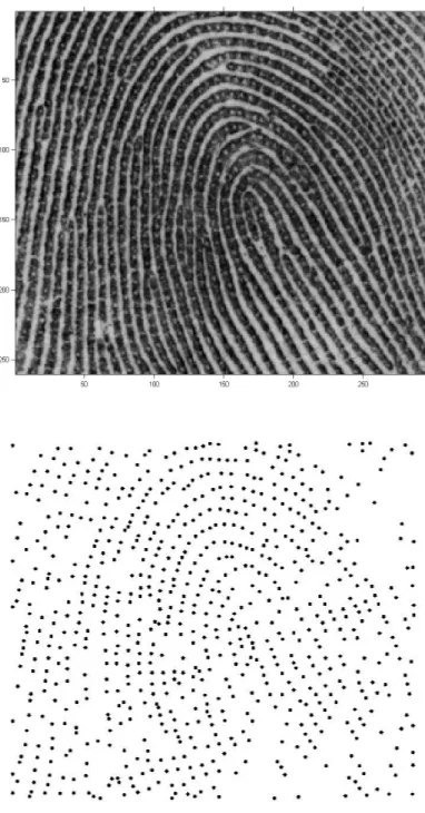
2.3 Fingerprint a002-05 and sweat pore pattern . . . 15

3.1 Simulated example of a point pattern arising from a fibre-process generated point process . . . 29

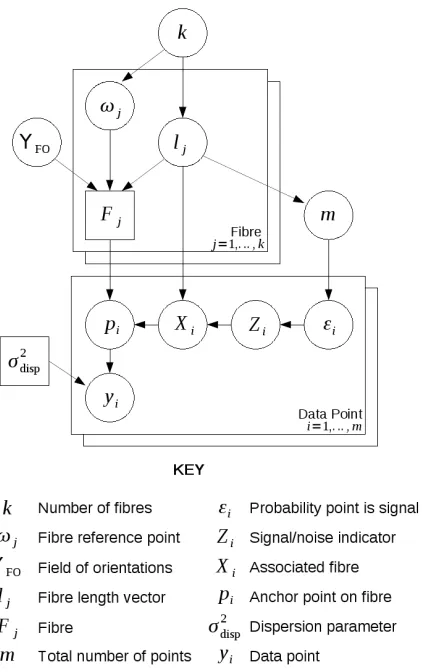
3.2 Directed Acyclic Graph (DAG) of model . . . 32

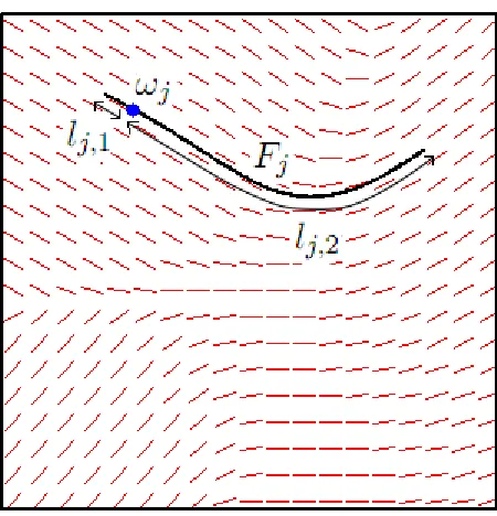
3.3 Fibre model construction . . . 33

3.4 Cropped window showing a large sample of fibres drawn from the prior fibre distribution . . . 39

3.5 A section of Figure 3.4 motivating the construction of a birth-death process . . . 40

4.1 Fingerprint a002-05 from the NIST database . . . 47

4.2 Pore data extracted from fingerprint a002-05 . . . 48

4.3 Four stages of the tensor method . . . 49

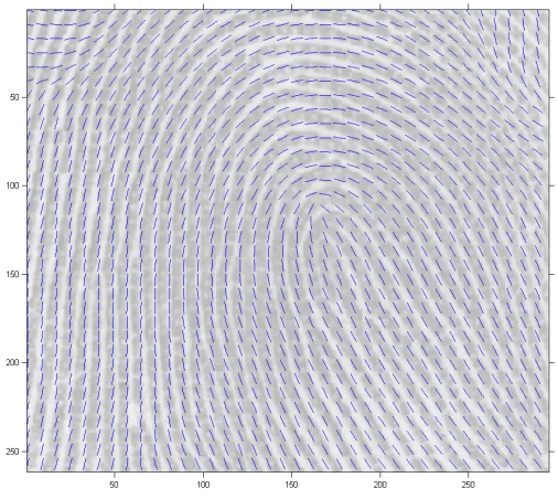
4.4 Principal eigenvectors of the tensors created by the tensor method . 50 4.5 Principal eigenvector field of the tensor field empirically estimated from the pore data . . . 55

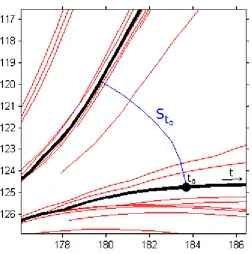
4.6 Orientations of the underlying fingerprint ridge-lines, around a circle centred at the loop of fingerprint . . . 56

4.7 Principal eigenvector field of the tensor field estimated withh= 10 . 57 4.8 Principal eigenvector field of the tensor field estimated withh= 60 . 58 4.9 A basic fingerprint structure of concentric arches . . . 59

4.10 The parabolic tensor field . . . 61

4.11 Main singularity of the interpolated tensor field for varying h . . . . 63

(9)

4.13 The principal eigenvector field of the bias-corrected tensor field

cal-culated by estimatingT0 fromTh with a Taylor series of order 2 . . 66

4.14 The principal eigenvector field of the extrapolated tensor field with parameters h1= 30, h2 = 60, andt= 3 . . . 68

4.15 The principal eigenvector field of the extrapolated tensor field with parameters h1= 30, h2 = 60, andt= 10 . . . 69

4.16 Field of orientations estimated using adaptive smoothing . . . 70

5.1 The two states involved in a split/join move . . . 93

6.1 Output figures for first simulated example . . . 108

6.2 Output figures for simulated example from Stanford and Raftery, 2000110 6.3 Trace plot of the number of fibres against algorithmic time for simu-lated data from Stanford and Raftery [2000] . . . 111

6.4 Output figures for earthquake data . . . 114

6.5 Trace plot of the total length of fibres across samples for earthquake data . . . 116

6.6 Output figures for fingerprint pore data . . . 117

6.7 Simulated helix data, viewed from 3 different angles . . . 120

6.8 Sample from the posterior distribution of fibres given simulated helix data . . . 121

6.9 Empirical estimate of the signal point process density given simulated helix data . . . 122

6.10 Subset of galaxy data . . . 124

6.11 Sample from the posterior distribution of fibres given the galaxy data 124 6.12 Empirical estimate of the density of signal points given the galaxy data125 7.1 Plot of various measures of anisotropy . . . 141

7.2 Contour plot for the probability that the nearest point to a signal point is also a signal point based on the linear fibre model . . . 144

7.3 Contour plot of the msF A of the mean tensor based on the parallel lines model for varying inter-fibre distanced . . . 145

7.4 Contour plot of the msF A of the mean tensor based on the parallel lines model for varying tensor parameter σ. . . 146

7.5 Contour plot of the msF A of the mean tensor based on the cosine Poisson process model for varying tensor parameter σ . . . 148

7.6 Anisotropy plot of simulated Stanford and Raftery data based on the initial tensors calculated using the tensor method at each point . . . 149

(10)

(11)

Acknowledgments

First and foremost, my deepest gratitude goes to my two supervisors, Elke Th¨onnes

and Wilfrid Kendall who have guided and supported me over the past four years.

I have learnt a great deal through working with both Elke and Wilfrid, from

de-veloping presentation and writing skills to gaining an inventory of techniques and

approaches to tackling problems.

I am grateful to the ˚Arhus Mathematics Department who funded my visit to

Den-mark and especially to Eva Vedel Jensen, Ute Hahn and Markus Kiderlen, for the

collaborative discussions and their kind hospitality.

I would also like to thank all the friends I have made throughout my PhD for

keep-ing me sane and makkeep-ing the years enjoyable. Special thanks go to Kat Abrahams,

Mouna Akacha, Leo Bastos, Maria Costa, Thais da Fonseca, Fla´avio Gon¸calves,

Stasia Grinberg, Ben Jacoby, Jason Laurie, Silvia Liverani, Chris Nam, Siren

Ve-flingstad, Peter Windridge and Piotr Zwiernik.

I am indebted to to my family who kept me going in the final few months by

providing a bit of perspective. Finally, I’d like to thank Richard Tyson for his

(12)

Declarations

I hereby declare that this thesis is the original work of myself, Bryony Hill. This

work builds on initial exploratory work by a previous PhD student (Su, 2009) that

investigates pore patterns in fingerprints and develops a basic approach to

estimat-ing ridge lines. Full attribution has been given to this author, and others, where

applicable.

Much of the new work of this thesis is summarised in Hill et al. [2011], including

the Bayesian model described in Chapter 3, and the tensor field calculation through

a kernel-smoothing interpolation, weighted by the probability that each point is

signal (see Chapter 4). The new anisotropy measure, the modified square Fractional

Anisotropy (msF A), proposed in Chapter 7 was motivated by joint work with Ute

(13)

Abstract

This thesis introduces a new approach to analysing spatial point data clustered along

or around a system of curves orfibres with additional background noise. Such data arise in catalogues of galaxy locations, recorded locations of earthquakes, aerial

images of minefields, and pore patterns on fingerprints. Finding the underlying

curvilinear structure of these point-pattern data sets may not only facilitate a better

understanding of how they arise but also aid reconstruction of missing data.

We base the space of fibres on the set of integral lines of an orientation field. Using

an empirical Bayes approach, we estimate the field of orientations from anisotropic

features of the data. The orientation field estimation draws on ideas from tensor

field theory (an area recently motivated by the study of magnetic resonance imaging

scans), using symmetric positive-definite matrices to estimate local anisotropies in

the point pattern through the tensor method. We also propose a new measure of anisotropy, the modified square Fractional Anisotropy, whose statistical properties

are estimated for tensors calculated via the tensor method.

A continuous-time Markov chain Monte Carlo algorithm is used to draw samples

from the posterior distribution of fibres, exploring models with different numbers

of clusters, and fitting fibres to the clusters as it proceeds. The Bayesian approach

permits inference on various properties of the clusters and associated fibres, and the

resulting algorithm performs well on a number of very different curvilinear

(14)

Chapter 1

Introduction

Spatial point patterns arise throughout nature as the locations of apparently random

objects or events. In statistical analysis, these data are commonly modelled as an

instance of a random point process, i.e. a random and locally finite collection of points. There is substantial literature on the statistical analysis of such point data,

however most research focuses on rotationally invariant orisotropicpoint processes. The work presented here is concerned with anisotropic point processes, in particular spatial point data clustered around a collection of curves or fibres.

The motivation for this thesis is the identification of systems of fibres generating

noisy point processes. Identification of curvilinear elements (i.e. point clusters

re-sembling curves) and elucidation of their relationship with the point data is both an interesting theoretical problem and a useful tool for gaining insight into the origins

of the data.

Point patterns exhibiting a filamentary structure often arise in nature when events

occur near some latent curvilinear generating feature. For example, earthquakes

occur around seismic faults which lie on the boundaries of tectonic plates and hence are naturally curvilinear. Similarly, sweat pores in fingerprints lie on the fingertip

ridges lines which have a curvilinear structure. Estimation of ridge lines from the

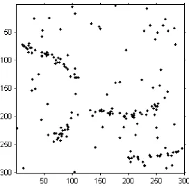
pore pattern could be used to develop a process for reconstructing smudged or patchy fingerprints. Figure 1 presents examples of these data together with two

simulated examples of point patterns clustered around underlying families of curves

with additional background noise. Our approach is flexible to the features of fibres, producing consistently strong results when applied to each of the four examples in

Figure 1; these results are presented in Chapter 6.

Other data exhibiting a curvilinear structure include land mines located on thin

(15)

(a) Simulated point pattern. (b) Simulated point pattern from Stanford and Raftery [2000].

(c) Earthquake epicentres in the New Madrid region. Data are taken from the earthquake catalogue at CERI (Center for Earthquake Research and Information).

[image:15.595.339.476.136.245.2]

(d) Pores along ridges of a sec-tion of fingerprint a002-05 from the NIST (National Institute of Standards and Technology) Special Database 30[Watson, 2001].

Figure 1.1: Four examples of point patterns clustered around latent curvilinear features with background noise.

around the edge of the Chicxulub crater on the Yucat´an Peninsula; and galaxies

that cluster in filaments around huge voids creating a 3-dimensional web-like

struc-ture. The detection of minefields is a high priority for defence forces, which has prompted investment from the United States Navy into project COBRA, the

de-velopment of purpose-built, unmanned reconnaissance aircraft (Witherspoon et al.,

1995). Estimation of the radius of the Chicxulub crater may clarify the extent to which the asteroid impact affected prehistoric life (Hildebrand et al., 2002).

Anal-ysis of the large-scale distribution of matter and identification of the 3-dimensional

cosmic web is a subject of great scientific interest, see Mart´ınez and Saar [2002] for further details. These data are described in further detail in Section 2.2.1.

The majority of the current approaches to estimating curvilinear features from noisy

(16)

associated point clustering. We show how properties of the underlying distribution

of fibres can be estimated using Monte Carlo techniques applied to the spatial point data. This approach has the significant advantage that it can be used to quantify

uncertainty on a range of parameters and does so effectively for different types

of curvilinear structure. The use of a field of orientations to identify fibres leads to a strong performance on data such as the fingerprint pore pattern shown in

Figure 1.1(d), despite the difficulty of there being noticeable alignment of points

perpendicular to the fibres.

The data in consideration typically arise from multiple fibres. Simultaneous

esti-mation of the number and location of the generating fibres is a difficult problem; existing approaches to estimating the number of isotropic clusters in a point

pat-tern are generally not-well suited to the long curvilinear clusters. Our approach uses

trans-dimensional Monte Carlo methods to explore the full posterior distribution of the set of fibres, thus models with different numbers of fibres can be compared

directly.

An important consideration in modelling fibre-generated point processes is the choice of state space for the random fibre process. There is no single natural choice for this

state space, although it is generally assumed that the random fibres are smooth and

continuous. A common approach is to approximate the smooth fibre by a piece-wise linear curve, however this results in the loss of the curvilinear details of the fibres.

The model introduced here describes families of non-intersecting curves via a field of orientations (a map from the window of observation W to [0, π) assigning an undirected orientation to each point in the window). The curves are identified by

segments of streamlines integrating the field of orientations. We say that a curve

integrates the field of orientations if the curve is continuous and its tangent agrees

with the field of orientations at each point. The termstreamlineis used to describe a curve which integrates the field of orientations and has no end points in the interior of the window W\∂W. This novel approach to modelling the generating fibre process permits, in principle, any smooth collection of non-intersecting fibres.

Note that we work with an orientation field rather than a vector field (a map from the window of observation W to [0,2π)). The distinction is drawn between the two in fingerprint analysis where a field of orientations is used to model the ridge lines,

see for example Ratha et al. [1995], and in engineering when studying the orientation of fibres forming in compressed fluids (Lee et al., 1997).

We choose to use a variant on an empirical Bayes approach to estimate the field of orientations, since a fully Bayesian approach would involve infinite dimensional

distributions and be computationally very intensive. The empirical Bayes

(17)

as detailed in Chapter 4. In this work, a tensor field is represented by the

assig-nation of a symmetric positive definite matrix to each point of the planar window. Tensor fields of this kind play an important role in diffusion tensor imaging (DTI),

as reviewed in Chanraud et al. [2010]. The field of orientations is constructed by

simply calculating the orientations of the representative matrices’ principal eigen-vectors; singularities in the field of orientations correspond to points where there is

equality of the two eigenvalues. This empirical Bayes approach enables the reliable

estimation of orientation fields (estimates are integrated by fibres producing high likelihoods), through the extension of previous work on tensors by Su et al. [2008],

Su [2009] and in diffusion tensor imaging (Dryden et al., 2009). Essentially,

ten-sors that estimate the local orientation of alignments in the point pattern data are smoothly interpolated to create a field of tensors; the orientation field is determined

from this tensor field.

The following chapter provides a background in the relevant areas of statistical analysis, together with an overview of existing approaches to solving the problem of

identifying filamentary structure in point pattern data. The original contributions of

this thesis begin in Chapter 3 with a full description of the proposed Bayesian model; details and justification of the empirical Bayes approach to estimating the field of

orientations are given in Chapter 4. Chapter 5 specifies the associated rates and

acceptance probabilities of a birth-death Markov chain Monte Carlo process (BDM-CMC) algorithm, which is used to draw samples from the posterior distribution of

fibres given a particular instance of the point process. Results of the

implementa-tion of our approach on the four data sets depicted in Figure 1 are presented in Chapter 6.

In Chapter 7 we return our focus to the positive-definite symmetric tensor, a

math-ematical object used in the orientation field estimation of Chapter 4 to summarise directional information in point patterns. This penultimate chapter describes how

tensors can be used to measureanisotropy, the extent to which a point process de-viates from isotropy. Here we propose a new measure of anisotropy, motivated by our choice of tensor estimator, the tensor method (Su et al., 2008 and Su, 2009). An analysis of the robustness of the tensor method is presented, and we propose

some potential applications of anisotropy measures in fibre-generated point pro-cesses. Possible areas for further research are suggested in Chapter 8, together with

a discussion summarising the work of this thesis. Much of this work is reported on

(18)

Chapter 2

Background and Related

Work

This thesis is primarily concerned with anisotropy (a lack of directional invariance) in

spatial point patterns. More specifically, it focuses on point processes that exhibit

curvilinear structure, with the aim of making inferences on the generating fibre process given an instance of the point process. This chapter presents an overview of

the relevant statistical theory for this thesis, together with a summary of existing

approaches to the analysis of fibre-generated point processes.

Section 2.1 provides some examples of how anisotropy can appear in point pattern data together with some of the known approaches to analysing this data. Anisotropic

point processes in which points are clustered around a number of curvilinear features

orfibres are described in Section 2.2. The aim of this thesis is to infer properties of

the fibres given an instance of such a point process. We appraise existing approaches

to solving this problem, and briefly discuss their strengths and limitations.

The treatment advocated in this thesis is based on the formulation of a general

Bayesian model for families of curves and the point patterns clustered around them.

Samples are drawn from the posterior distribution of fibres using a birth-death Markov chain Monte Carlo (BDMCMC) process. Section 2.3 gives an introduction

to fully Bayesian and empirical Bayes techniques, together with an overview of

relevant work in Markov chain Monte Carlo methods.

An important consideration in the formulation of the model is how to define the

random fibre process. We choose to model fibres as segments of streamlines that integrate a smoothfield of orientations υFO:W →[0, π) where [0, π) represents the

(19)

This thesis builds on the initial exploratory work of Su et al. [2008] (see also the

ear-lier PhD thesis Su, 2009), which is motivated by the fingerprint pore data. Positive-definite symmetric matrices ortensors are used to produce local estimates of point pattern orientations. These tensors form the basis of an empirical Bayes estimation

of the field of orientations. Tensors of this form, discussed in 2.5, are used in a range of disciplines to summarise directional information. We describe the uses of

tensors in diffusion tensor imaging, a technique in magnetic resonance imaging that

has recently stimulated research into tensor analysis, with similar aims to our own. Particular reference is made to current work on the different metrics prescribed for

tensors.

2.1 Anisotropy in Spatial Point Processes

We briefly describe the notion of a point process, provide a few examples of anisotropic point processes, and list some available approaches for analysing anisotropic point

patterns. The focus of this thesis is on anisotropic point patterns that exhibit

curvi-linear structure, which are discussed in Section 2.2.

A spatial point process is defined in Stoyan et al. [1995] as a random collection of

points in Rn, which is locally finite (each bounded subset contains a finite number

of points) and contains no repeated points. We focus primarily on planar point

processes overR2, but many ideas extend naturally to higher dimensions.

Inter-point distances and the local density of spatial point processes have been studied in some detail; Ripley [1981] and Diggle [1983] describe a number of the

statistics typically used. The hypothesis that a point pattern is an instance of a

homogeneous Poisson point process can be tested using such statistics. They are also helpful for identifying other structures in the point pattern, such as clustering

or regularity. However, discussions are usually restricted to stationary (invariant

under translation) and isotropic (invariant under rotation) point processes.

A point processes is said to exhibit anisotropy if it is not invariant under rotation.

Anisotropy may appear in different forms including the local alignment of points,

and global structures, such as anisotropic clusters of points. The focus of this thesis is on the second of these two types of anisotropic point processes, specifically those

that exhibit clusters in the form of curvilinear features. This type of point process

is described in Section 2.2.

First, we provide a few examples of where such point patterns can be found in

nature, followed by an overview of existing approaches to studying anisotropy in

(20)

[image:20.595.162.401.106.341.2]

Figure 2.1: A simulated example of a Glass pattern using an exponential transfor-mation.

2.1.1 Examples from Nature

It is suggested (Guan et al., 2006) that the locations of certain shrubs in the North

American Mojave desert are directionally associated. Surviving seedlings tend to lie

on the north side of existing shrubs where shadow keeps the soil from drying.

Illian et al. [2008] provide two further examples of anisotropy. The first is of 573 carbide particles in rolled steel that tend to cluster in bands parallel to the direction

of the rolling. The second example is of two proteins on the surface of a cell that

appear to be aligned in pairs of proteins, one of each type, with pairs similarly oriented across the cell.

2.1.2 A Simulated Example - Glass Patterns

Glass patterns, named after the physiologist Leon Glass (see Glass, 1969), consist

of a random set of points, superimposed with a geometrically transformed copy. An example is displayed in Figure 2.1. By looking at the point pattern the brain can

easily visualise the underlying pattern. These patterns are predominantly used for

investigations into psychophysical study of how the brain perceives form. However, they also provide an interesting example of anisotropy in point patterns, and are

of particular note as they have a locally parallel structure, similar to the pores on

(21)

Section 2.1.3 describes how Stevens [1978] proposed to identify local orientations in

Glass patterns.

2.1.3 Testing for Anisotropy and Estimating Orientation

This section briefly describes some of the existing approaches to analysing anisotropic point patterns.

Nearest neighbour methods, the analysis of second-order orientations and the rose

of directions provide the basis for tests of anisotropy and the determination of the global dominant orientation of a point pattern. Steven’s method supports the

esti-mation of local orientation within a point pattern.

This thesis uses methodology based on the tensor method, an extension of kernel

principal components analysis (kPCA), to estimate local orientations of a point pattern.

Nearest Neighbour and Second-Order Orientation Analysis

Illian et al. [2008] suggest exploring the distribution of the orientations of line

seg-ments that connect each point to its nearest neighbour. This is appropriate for

identifying local anisotropy (and its direction) where the direction of anisotropy is constant throughout. However, if the direction of anisotropy varies (e.g. in the

Glass pattern of Figure 2.1), or arises from anisotropic clusters, this approach is less

effective.

A second-order orientation analysis, also described in Illian et al. [2008], is used to explore the distribution of orientations of line segments connecting pairs of points

with an inter-point distance lying in some interval [r1, r2]. The values r1 and r2

are usually found by experimentation. This approach is rather more suitable for investigating anisotropic clusters which exhibit anisotropy on a larger scale, such

as the 573 carbide particles in rolled steel described previously. However, a global estimate of the orientation of line segments is less informative when the data exhibits

anisotropy that varies in orientation.

The distribution of these orientations is equivalent to therose of directions (Stoyan et al., 1995) of the line process given by the collection of lines between pairs of points whose lengths lie in the interval [r1, r2], as described in Su et al. [2008]. The rose

of directions was primarily developed for use in hypothesis testing and is therefore

(22)

Steven’s Method

Stevens [1978] is concerned with the visual processing of point patterns in artificial

intelligence, and makes the following hypothesis about Glass patterns.

One perceives in these patterns a structure that is locally parallel. Our

ability to perceive this structure is shown [...] to be limited by the local

geometry of the pattern, independent of the overall structure [...]

This idea relates to our approach where the local relative orientation of points is

considered first, then interpolated to estimate the global structure.

Steven’s method, an extension of the second-order orientation analysis that produces

local estimates of dominant orientation in a Glass pattern, proceeds as follows.

A histogram approach is used to produce local estimates of the rose of directions

for the lines connecting pairs of points. Each local estimate is based on the lines connecting all pairs of points within a disc (of predetermined fixed radius) centred

at a point. The dominant orientation is estimated by smoothing the histogram and

choosing the peak of the resulting distribution.

The algorithm presented in this paper produces an effective estimator for the local

orientations in Glass patterns, however this approach was not designed for mak-ing more general inferences on the properties of an underlymak-ing random point

pro-cess.

Kernel Principal Components Analysis and the Tensor Method

A principal components analysis or PCA (see, for example, Marriott, 1974) is a

technique for reducing the dimensionality of a data set by transforming the data to

a new coordinate system. Under the new coordinate system, the first coordinate (or firstprincipal component) indicates the direction that maximises the variance of the data projected onto the equivalent axis. Each subsequent principal component

is orthogonal to all previous components, but similarly maximises the variance of the projected data. A subset, usually the first k principal components for some

k < n (n being the dimensionality of the data) are proposed as a new basis for the data.

The principal components are found by identifying the eigen-decomposition of the

empirical covariance matrix calculated from the mean-centred data. Specifically, the first coordinate is indicated by the principal eigenvector (with the largest

corre-sponding eigenvalue), and further principal components are given by the eigenvectors

(23)

Kernel principal components analysis or kPCA (Sch¨olkopf et al., 1997) is the

ex-tension of principal components analysis where the data is first projected on to a different coordinate system, usually of a higher dimension. This permits the

detec-tion of nonlinear trends in the data.

The data y1, ..., ym ∈ RN are mapped into feature space F by the function Φ : RN → F. In principle, the analysis proceeds following the linear PCA approach

on the transformed data Φ(y1), ...,Φ(ym), i.e. eigenvectors v and eigenvaluesλ are

found satisfying

Cv=λv (2.1)

where C= 1

m

X

i=1

Φ(yi)TΦ(yi). (2.2)

The dimension of covariance matrix C could be arbitrarily large, depending only

on the dimension of feature spaceF. For this reason the problem is restated as the eigen-decomposition of an N-dimensional matrix, specifically the ‘kernel’ matrix, defined in terms of a kernel functionk(·,·),

Ki,j =k(yi, yj) := Φ(yi)·Φ(yj) (2.3)

(recall N is the dimensionality of the data). We briefly describe the motivation for using the kernel matrix and how the corresponding eigenvectors and eigenvalues

relate to the data.

First note that any eigenvectorvsolving Equations (2.1) and (2.2) must be spanned

by the vectors Φ(y1), ...,Φ(ym), i.e.

v=

m

X

i=1

αiΦ(yi). (2.4)

Therefore, consider instead the following system of equations:

Φ(yk)·Cv= Φ(yk)·λv for allk= 1, ..., m. (2.5)

(24)

1, ..., m

Φ(yk)·

1

m

X

j=1

Φ(yj)TΦ(yj) m

X

i=1

αiΦ(yi) = Φ(yk)·λ m

X

i=1

αiΦ(yi)

1 m m X j=1 m X i=1

(Φ(yk)·Φ(yj)) (Φ(yj)·Φ(yi))αi =λ m

X

i=1

Φ(yk)·Φ(yi)αi. (2.6)

Alternatively, this can be written in matrix form using the kernel matrixKdefined in Equation (2.3) and writing the vector (α1, ..., αm)T asα:

1

mK

2_α₌_λ_K_α_. _(2.7)

Solutions of Equation (2.7) can be found by solving

1

mKα=λα, (2.8)

for α. The projection (Φ(x)) of the image of a point x onto the k−th eigenvector vk is given by

m

X

i=1

αk_iΦ(yi)·Φ(x) (2.9)

where αk_i is the i-th element in the k-th eigenvector. Hence the projection Φ(yi)

need not be directly calculated, just the kernel function,k(x, y) = Φ(x)·Φ(y).

Examples of typical kernel functions include

k(x, y) = (x·y)d (polynomial kernels), (2.10)

k(x, y) = exp(||x−y||2_/₂_σ2₎ _{(radial basis functions),} _(2.11)

and k(x, y) = tanh(a(x·y) +b) (sigmoid kernels). (2.12)

The advantage of posing the problem as the eigen-decomposition of kernel matrix K rather than the covariance matrix C is that we can choose a high-dimensional

feature space with little impact on the computing time required. If the size of the dataset is very large, the data may be de-noised as in Minier and Csat´o [2007], or

by partitioned into smaller subsets (see for example Shi et al., 2009) to reduce the

dimensionality of kernel matrixK.

This approach to principal components analysis allows the extraction of nonlinear

features from data. The drawbacks are that it is generally not possible to calculate

(25)

non-trivial, and that the dimension of the matrix to be eigen-decomposed grows

with the number of data. It is also worth noting that kPCA requires some prior knowledge of the nonlinear features to be extracted, although the scope of this class

of features is controlled only by the dimensions of the feature space which may be

arbitrarily high at a low computational cost.

In this thesis, we build on the work of Su [2009] and Su et al. [2008], where the tensor method, a variant on kPCA, is used to estimate the local orientations of a point pattern. The termtensor is used to describe the sum of the outer product of each vector representing a data point with itself. An overview of tensors is given at the end of this chapter.

The tensor method proceeds as follows. Let P1, ..., Pn denote the points in an

in-stance of a point process. A tensor is created at pointPj by applying a non-linear

transformation to the vectorsvi = (vi₁, v₂i) =−−→PjPi fori6=j. Specifically,

˜

vi = (˜v₁i,˜vi₂) = exp − (v

i

1)2+ (v2i)2

/2σ2 q

(vi₁)2_{+ (}_vi

2)2

(vi₁, v₂i) (2.13)

whereσ is a scaling parameter. The Gaussian transformation was chosen because it is continuous, decreases with distance, and the properties of the Gaussian function

are well understood.

The tensor atPj is then calculated by

T(Pj) = 2

X

i6=j

(˜vi₁,v˜i₂)T(˜vi₁,v˜i₂). (2.14)

The multiple of 2 arises because all vectors ˜vi are copied and rotated 180 degrees aboutPj to centre the mean of the transformed vectors.

Two main differences between the tensor method and kPCA are: (1) - in kPCA

the equivalent to the sum in Equation (2.14) is over the vectors between all pairs of

points rather than just those including the pointPj; (2) - the tensor method omits

the normalising constant 1/(n−1), therefore as the number of points increases, so does the ‘size’ of the tensor.

As with kPCA, the tensor’s principal eigenvector gives the principal axis along which

the variance of the transformed points are maximised. Hence if the untransformed vectors vi were projected onto the principal axis, their endpoints (the locations of

Pi) would lie relatively close to the initial pointPj suggesting that the principal axis

(26)

2.2 Curvilinear Features in Point Processes

We now focus our attention on a particular class of anisotropic point process, those containing long, thin, curved clusters.

A fibre process is a random collection of curvilinear geometric objects; it is a natural

generalisation of a line process (see Stoyan et al., 1995). Interest in the literature

focuses on the stationarity of fibre processes and the number of intersections with lines or other objects. Stationary fibre processes are often described in terms of

their intensity (mean length per unit area) and the rose of orientations given by the

orientations of the tangents to the fibres.

A fibre-process generated Cox process is a Poisson point process whose driving

in-tensity measure relates to a random fibre process. The name originates from Illian

et al. [2008] who present the example of a Poisson point process along an instance

of a random fibre process, with intensity λf points per unit length of fibre.

In this thesis we consider the more general fibre-process generated Cox process where points are distributed around fibres rather than along them. This type of

point process is further generalised to fibre-process generated point processes, that depend on a fibre process without the restriction of being Poisson-distributed.

2.2.1 Example Data Sets

Point patterns with a filamentary structure exist in many different areas of study and at greatly varying scales. Some examples are provided below.

Earthquake Epicentres

Earthquake epicentres are typically clustered around an underlying curve structure

defined by seismic fault lines. An illustration of the clustering of earthquake epi-centres around the world is can be found athttp://pubs.usgs.gov/gip/earthq4/

severitygip.html. There is some interest in using statistical methods to describe

the underlying structure, particularly in the principal curve analysis described in Stanford and Raftery [2000].

Minefields

The need to locate minefields before and during assaults makes minefield detection a

(27)

mines as well as a number of miscellaneous objects or artefacts of a region of interest.

This is studied in papers such as Cressie and Collins [2001] and Fraley and Raftery [1998], although currently most published work is only applied to simulated data.

The simulated data typically consists of homogeneous Poisson processes on multiple

wide strips superimposed on background noise. An example is presented in Figure 2.2. As such, approaches to identifying the minefields generally take no account of

the anisotropy or filamentary nature of the point process, partly because it is not

[image:27.595.210.428.250.471.2]

evident on a local scale.

Figure 2.2: A simulated example of minefield data. Dots indicate objects detected through reconnaissance imagery; the dense region of points is suggestive of a mine-field.

Pores in Fingerprints

Fingerprints are widely used in forensics, biometric identification and security sys-tems. They have benefits over other forms of biometric identifier (e.g. iris scanning,

DNA testing, voice recognition) of being unobtrusive, highly distinctive, relatively

permanent and easily collectable (Maltoni et al., 2003). As a result, there has been a large amount of research into the investigation of claims of individuality of

fin-gerprints, creating new recognition and classification systems, and building high

resolution fingerprint scanners that capture all the fingerprint details.

Sweat pores are tiny holes along the ridge on a fingertip where the ducts of the

sweat glands open. The underlying fibre structure is the dense set of approximately

(28)

usually close to the centre of the ridge (see Figure 2.3).

Ridges on fingertips usually form concentric patterns with loops and/or arches,

which help to resist slipping in all directions (particularly concentric patterns). The ridges are constructed from ridge units, each having one sweat gland and one pore

opening at some point on its surface. Consequently the distance between adjacent

[image:28.595.184.375.249.614.2]

pores on a ridge appears to be proportional to the width of the ridge (see Ashbaugh, 1999).

Figure 2.3: Top: Fingerprint a002-05 from the NIST Special Database 30 (Watson, 2001). The sweat pores appear as small light-coloured circles along the ridges. Bottom: The pore pattern of fingerprint a002-05, identified using empirical image analysis techniques (see Su et al., 2008).

An example of a fingerprint and the pattern of pores extracted from it are presented in Figure 2.3. The curved structure of the fingerprint ridge lines is clearly discernible

from the pattern of sweat pores shown in the second figure.

(29)

noise, has potential for aiding reconstruction of patchy fingerprints and may also

allow for more efficient storage of fingerprints in huge databases.

Cenotes

A third geographical example is of cenotes (surface connections to underground

water bodies), typically found in the Yucat´an Peninsula where they are clustered

along the circumference of the Chicxulub crater. The cenotes are clustered around just one curve, with non-uniform background noise.

Galaxies

A final application, extending the problem to 3 dimensions, is that of the locations

of galaxies in the universe. Galaxies tend to cluster along filaments forming a 3-dimensional web-like structure with large voids between the filaments. In this

application the points are clustered around a large number of intersecting curves.

Mart´ınez and Saar [2002] describe a number of the statistical methods used to analyse the large-scale structures; however the focus of this thesis is on 2-dimensional

data.

A simulation of the web-like cosmic structure can be found athttp://cosmicweb.

uchicago.edu/filaments.html.

Varying Features of Data

The above examples exemplify the variety of features that can be found in this type

of data. They have different numbers of curvilinear features, which, in turn, are of

varying curvature and thickness. Where multiple curvilinear features exist they may be densely packed or sparsely located, and they can be locally parallel (as in the

fingerprint pore data) or connect in the web-like structure of the galaxy data. There

are also different types of background noise (e.g. homogeneous, clustered).

The approach described in this thesis is flexible enough to draw inferences on most

of these types of data, although it is restricted to fibres that do not cross.

2.2.2 Existing Approaches

Of the existing approaches to identifying curvilinear clusters in background noise,

(30)

One such approach involves finding the Voronoi tessellation of the point pattern.

This is the set of regions that partitions the window of observation (or R2) such

that any point in the space is in the same region as the nearest data point, and no

two data points are in the same region. These regions are called Voronoi polygons

as they are necessarily polygons for a finite point pattern.

Allard and Fraley [1997] propose a method for detecting the support domain of a

uniformly distributed point pattern within a second uniformly distributed point pat-tern with a larger support domain. They simply take the union of Voronoi polygons

that maximises the likelihood of their model. This approach has the advantage that

it can be adapted for any shape of point cluster. However, if geometrical constraints such as the number of clusters are made then the maximum likelihood estimator

can only be approximated. Also, as with most of these approaches, only a point

estimate of the underlying structure is obtained.

Byers and Raftery [1998] propose a method for detecting features in noisy point

pattern data, using the distance to the K-th nearest neighbour to separate dense point clusters from the background noise. This produces similar results to the

Voronoi tessellation approach of Allard and Fraley [1997], but leads to a classification

of points to noise or signal rather than identifying a union of regions in which the feature is expected to lie. While this approach is easily extended to higher

dimensions, it is based on the assumption that the signal point pattern is an instance

of a Poisson process. Byers and Raftery [1998] also note that the parameterKneeds to be chosen with some care.

The following approaches to analysing anisotropic point patterns put a greater focus on identifying the curvilinear structure.

Density-Comparison Approaches

A piecewise linear Candy Model is used by Stoica et al. [2005] to model filaments in galaxy data, and extended to the 3-dimensional Bisous Model in Stoica et al. [2007]. The Candy Model comprises of random linear objects or network segments that ‘link’ under certain conditions (such as proximity and relative orientation) to

form a collection of networks, with connected filamentary structure.

To fit the model to the data, the empirical densities of galaxies in two disjoint

regions are compared. The first region is the interior volume of the linear object, and the second is a region surrounding the linear object. Linear objects are more

likely to be accepted as part of the filamentary structure if the density is higher

(31)

the densities of points in concentric cylinders. An energy function is defined for

a network of segments, and a simulated annealing approach is used to determine the network that minimises this energy. This approach is restricted to piecewise

linear fibre models, the lengths of the linear segments being limited by the density

of points.

A similar approach to the Candy Model is proposed in Arias-Castro et al. [2005] who consider the detection of filamentary structures in point patterns over the [0,1]×[0,1] square. In particular they test whether the point pattern, consisting mainly of points

distributed uniformly at random over the unit square, also contains a set of points sampled from a continuous curve. Note that in this instance the signal points are

assumed to lie directly on the curve or fibre.

They proceed by counting the number of data points that lie in thin regions or strips and accepting each strip if it contains more than a certain number of points.

Accepted strips are connected if they satisfy certain continuity properties. The null

hypothesis that the unit square contains no fibre-dependent points is rejected if the total length of the accepted strips exceeds a predetermined threshold. As is

mentioned, this approach does not consider the estimation of the fibre, only the

detection to see if one actually exists.

The strips are defined as functions y = f(x) under a Cartesian coordinate system (x, y). Hence, as it stands, the currently proposed method is not rotationally in-variant and will not detect some curvilinear structures, although Arias-Castro et al. [2005] have suggested an extension to solve this problem.

Path-Density Approach

A density estimator of the point pattern can be obtained using techniques such

as kernel smoothing. Kernel smoothing is a statistical methodology for describing

point data by a curve or surface, and is commonly used to estimate the density function given a data sample. The kernel density estimator at a point x is given by

ˆ

f(x;h) = 1

nh

n

X

i=1 K

(x−yi)

h

, (2.15)

wherey1, ..., ynare a data sample, andK(·) is a kernel, typically a positive function

of the distance between two points that decreases with increasing distance, with

bandwidth parameterh. See Wand and Jones [1995] for further details.

Fibres can be directly estimated from this density; an example of this can be seen

(32)

constructed and the density of these paths is considered an estimator for the density

of an underlying fibre process.

The data are modelled as an inhomogeneous Poisson process with density described by a mixture of three components: curves, clusters and background noise. The

component arising from fibres is modelled as the convolution of a Gaussian kernel

with the fibre; clusters are the equivalent of zero-length fibres. They proceed to show that the paths of steepest ascent (of the empirical estimate of the point process

density) concentrate near the fibres of the model. A second kernel smoothing is

applied to the paths providing an estimator of the underlying fibre process.

While this technique is an improvement over other approaches that only provide a

point estimate of the curvilinear features, it has the shortcoming that it does not

implicitly classify points into noise and signal components or support inference of the properties of individual fibres (such as lengths, curvature, etc.). Examples show

that the main curvilinear clusters are identified, however, the approach leads to

density estimates that require trimming or choosing high level sets. It is also rather sensitive, in that it often identifies artefacts from the background noise as potential

clusters.

Minimal Spanning Trees and the Skeleton Model

A further approach discussed in Barrow et al. [1985] is based on the construction of

the minimal spanning tree of the point pattern. A spanning tree is a set of points

and edges (lines between pairs of points), such that all points are included and con-nected (through paths of edges), and no loops (closed paths) occur. The minimum

spanning tree is the spanning tree with minimal total edge length. Reducing the

minimum spanning tree, by ‘pruning’ or removing edges if they fail to meet certain requirements, leaves a simple tree describing the filamentary structure of the point

data. It is particularly useful in three dimensions, where it provides a useful insight

into the overall characteristics of the filamentary structure. However, it does not provide the means for much further inference and relies on an appropriate choice

of the level of pruning. It is also unsuited to walls of galaxies (points aligned in 2-dimensional surfaces in 3-dimensional space).

An alternative to the minimal spanning tree is proposed in Novikov et al. [2008],

where a skeleton model is used to describe the structure of a density estimate of a

point process. A smooth density estimate is found by applying a kernel smoothing to an instance of the point process. The skeleton is formed by considering curves

perpendicular to the iso-contours of the smooth density field, originating from local

(33)

random field.

Both of the above approaches are well adapted for identifying branching or

bifurca-tion of fibres, an important aspect of galaxy data, and an aspect that is ignored in our approach.

Principal Curves

An existing method for estimating the curves in the underlying structure of a point

process is Stanford and Raftery [2000]’s use ofprincipal curves(Hastie and Stuetzle, 1989), a nonlinear generalisation of the first principal component line. Specifically,

a principal curve of a densityh is defined as a curvef, parameterized by arc-length

λ, such that

E[X|fλ(X) =λ] =λ (2.16)

for almost allλ, where Xis a random vector with densityh, andfλ(X) is the value

of λsuch that f(λ) is the orthogonal projection of X onto f. The principal curve is fit to the data by iteratively applying this definition.

The approach is based on the assumptions that the background noise arises as a

homogeneous Poisson process and features in the point pattern are modelled by nor-mally distributed orthogonal perturbations from points uniformly distributed along

unknown curves (identified as cubic B-splines). The features are then combined in

a mixture model.

For each combination of number of components and degree of smoothness an opti-mal clustering of points is estimated. A classification version of the

Expectation-Maximisation algorithm is used to cluster the data into features that maximises the

likelihood of the model, and simultaneously fit principal curves. An optimal choice of smoothness and number of components is then selected using Bayes factors.

This technique generally performs very well; however it is sensitive to the initial

clustering of the data in the Expectation-Maximisation algorithm, and also has difficulties reconstructing fibres where signal points are sparse (for example the

fingerprint pore data - Figure 2.3). The authors also mention that a lower bound

on the variance of the perturbation of points from curves must be chosen, otherwise the principal curves may be over-fitted.

The remainder of this chapter describes some of the statistical theory and

methodol-ogy drawn upon within the thesis. Brief explanations are provided here; for a more

(34)

2.3 Bayes, Empirical Bayes and Markov Chain Monte

Carlo

The approach proposed in this thesis involves modelling the point process using a Bayesian hierarchical model as formulated in Chapter 3. An empirical Bayes

approach is used to estimate the prior of the field of orientations (used to describe fibres) from the data. Properties of the posterior distribution of fibres, conditional

on the data, are then estimated using Markov chain Monte Carlo methods.

This section briefly describes how such Bayesian inference proceeds.

2.3.1 Bayesian Inference

Bayesian inference involves estimating features of the posterior distribution deter-mined by Bayes’ Theorem (Bayes, 1763) as

f(θ|y) = R f(θ)L(θ|y)

f(θ)L(θ|y) dθ, (2.17)

where θ are the parameters of interest, y is the observed data, f(θ) is the prior on θ and L(θ|y) is the likelihood function. By sequentially using Bayes theorem, a hierarchical model of priors and hyperparameters is created. This permits great flexibility and allows the propagation of uncertainty throughout the model.

Ad-vances in computing over the last 20 years have made it easier to study complex

Bayesian models.

Through Bayes’ Theorem, point estimates and confidence (or credible) intervals of the posterior distribution of parameters given the data can be found.

2.3.2 Empirical Bayes

Empirical Bayes, a term coined by Robbins [1964], means that the prior distribution

(or a Bayes decision rule) is estimated directly from the data. It is argued that all Bayesian methods are empirical as, when postulating the prior, the data is almost

always taken into consideration. However, the term empirical Bayes methods is used to describe a more rigorous framework in which these empirical estimates are made.

As described in Maritz and Lwin [1989], an empirical Bayes approach is typically

implemented when the same experiment is executed repeatedly generating a series

(35)

previous components can be used in the calculation of the posterior distribution for

the current component. The data are used to estimate the prior distribution, or alternatively the Bayes decision rule is directly estimated from the data. Empirical

Bayes is an approximation to the fully Bayesian approach described in the previous

section.

Criticisms of the empirical Bayes methodology include that it uses the data twice, contradicting the Bayesian philosophy (Gelman, 2008). It also assumes

exchange-ability of the data components, which is not always reasonable.

It is usually assumed that a hyperparameter η is unknown but can be estimated from the data. The empirical Bayes approach involves estimating this parameter using the marginal distribution of the data,

Z

L(θ|y)f(θ|η) dθ. (2.18)

Hereyis the data, andθdenotes all other unknown parameters with joint prior

den-sity functionf(θ|η), conditional on hyperparameterη, and likelihoodL(θ|y).

In parametric empirical Bayes methods (see Carlin and Louis, 2008) it is assumed that there is a family of prior distributions F(θ|η) indexed by η. The parameter

η is then estimated (for example, as a maximum likelihood estimator) and plugged back into Equation (2.18) to estimate the posterior distribution.

Empirical Bayes methods reduce the bias in the posterior density associated with choosing hyperparameters. However, it should be noted that empirical Bayes

con-fidence intervals such as highest posterior density intervals often have insufficient

coverage, or are too short. This is because they do not account for the uncertainty in the posterior distribution induced by estimating the hyperparameter.

2.3.3 Markov Chain Monte Carlo

Markov chain Monte Carlo (MCMC) methods, which have been used extensively

over the past 50 years in statistical physics, are now commonly used in statistics for estimating properties of posterior distributions in Bayesian models.

MCMC methods allow us to draw samples from the posterior distribution without

the need to fully evaluate the normalising constant,

Z

f(θ)L(y|θ) dθ. (2.19)

(36)

of these samples.

The idea behind MCMC sampling is that a Markov chain can be constructed, that

will explore the state space, and has stationary distribution equal to the target

distribution - in this case, the posterior distribution. The Markov chain is typically constructed by proposing moves and accepting or rejecting them according to some

calculated probability.

A popular choice of move is the Metropolis-Hastings update. An update θ0, of one or more variables θ, is proposed from the proposal density Q(θ0|θ) and accepted with probability

α= min

1,π(θ

0₎_Q₍_θ_|_θ0₎

π(θ)Q(θ0_|_θ₎

, (2.20)

where π(·) is the target distribution. If the proposal density is symmetric, i.e.

Q(θ0|θ) =Q(θ|θ0), then the terms cancel leaving a Metropolis update, with accep-tance probability

α= min

1,π(θ

0₎

π(θ)

. (2.21)

Brooks et al. [2011] provides a recent overview of MCMC methods.

In Chapter 5, MCMC methods are used to sample from the posterior distribution of

parameters (including fibres) given the data points. As already identified, our model has the flexibility of not fixing the number of fibres (or point clusters), and so we

require a type of MCMC method that enables the exploration of states with different

numbers of fibres. This is referred to as a variable dimension problem, and the two main solutions are Reversible-Jump MCMC and Birth-Death MCMC (collectively

termed trans-dimensional MCMC, see Roeder and Wasserman, 1997).

Reversible-Jump MCMC or RJMCMC is proposed in Green [1995] and extends the

Metropolis-Hastings update to a move that varies the number of parameters in the model. Birth-Death MCMC or BDMCMC is a continuous-time approach to the

variable dimension problem, and is an extension of the more general birth-death

process (see Preston, 1977). RJMCMC and BDMCMC are very similar, indeed a sequence of RJMCMC samplers can be shown to converge to a BDMCMC under an

appropriate rescaling of time; see Capp´e et al. [2003] for further details.

Reversible-Jump MCMC

(37)

probabil-ity

α = min

1,π(k

0_{, θ}0₎_Q₍_k_|_k0₎_Q₍_u0₎

π(k, θ)Q(k0|k)Q(u)

∂g(θk, u)

∂(θk, u)

, (2.22)

whereQ(·) denotes a proposal density and u, u0 are the vectors of random variables such that a bijective function (θ0, u0) =g(θ, u) maps the current state to the proposed state see Green [1995] for further details.

The bijective function and random variables can be chosen to create pairs of moves such as birth and death, where a component is created or destroyed without directly

affecting the other components, or split and join, where one component is replaced by

two similar components, or two components replaced by one, described in Richard-son and Green [1997]. These dimension-jump moves, together with moves within a

fixed dimension (e.g. Metropolis Hastings updates), form a RJMCMC.

Birth-Death MCMC

The BDMCMC as described in Stephens [2000a] is an extension of the spatial Birth-Death process described in Ripley [1979]. As with the RJMCMC, it is used to draw

samples from a posterior distribution with an unknown number of components,

however, here the time scale is continuous and events occur at a predetermined or calculated rate. As is evident from the name, the two main types of event are birth

and death moves.

During a birth move a component is proposed from some birth density, and during

a death move a component is deleted. This is similar to RJMCMC, the main

differ-ence being that rather than proposing and then accepting or rejecting moves, the events are proposed at varying rates and always accepted. Hence, the rates of birth

moves and the death rates of components are chosen so that detailed balance holds

and the limiting distribution of the chain will therefore be the target distribution. Rejection sampling is sometimes incorporated into the birth proposal where it is not

feasible to draw samples directly from the birth density. Other moves, can also be

proposed at some rate using Metropolis-Hastings probabilities to accept or reject them, for example, split and combine (join) moves are implemented in Capp´e et al.

[2003].

There is an issue with processing the output of RJMCMC and BDMCMC, known

as the label switching problem (see Jasra et al., 2005), in that it is not trivial to identify components across samples. Hence, the marginal distribution of parameters of individual components are often unidentifiable. One approach to solving this

problem is to put artificial identifying constraints on the components as described in

(38)

output statistics. Suppose each component is identified by some parameterµi with

the constraintµ1 < µ2< ... < µi < ..., then estimates ofµi calculated from a series

of MCMC output samples would be ‘pushed apart’. This is because, in estimating

µ1 for example, we are estimating the random variable taking the minimum value of

all component means, rather than the mean value of the component believed to have the lowest mean. Stephens [2000b] provides a brief overview of existing solutions to

this problem.

There is particular difficulty in choosing convergence diagnostics for RJMCMC and

BDMCMC as most parameters, on which convergence diagnostics are typically based, are non-identifiable across samples. The approach described in

Richard-son and Green [1997] is to test the number of components k for convergence, and then test the convergence across samples with fixed k. This has the disadvantage that models with a particular number of components may be so infrequently

sam-pled that it is difficult to determine whether they have converged. Both Brooks and

Giudici [1998] and Castelloe and Zimmerman [2002] suggest alternative convergence diagnostics suitable for RJMCMC, based on the work of Gelman and Rubin [1992],

that compare the variation of a random variable between chains, within chains, and

between models.

Full details of the BDMCMC algorithm are provided in Chapter 5.

The two final sections of this chapter describe two mathematical objects - thefield of

orientationswhich is instrumental in our construction of a random fibre process; and

thetensor, used in the empirical Bayes estimation of the field of orientations.

2.4 Field of Orientations

We define a field of orientations (or simply an orientation field) as a map νFO

from the window of observation W to the interval of orientations [0, π), where 0 is associated with π. The interval of orientations corresponds to the collection of points on a circle of unit radius where antipodal points are equivalent. Thus, the

field of orientations can be thought of as the scalar field obtained by projecting a

vector field onto the half unit circle.

The integral curve of a field of orientations is defined as a map γ : I → W where

I is a real interval, and

∂γ(t)

∂t

=|υF O(γ(t))|. Theory from dynamical systems (see,

for example, Irwin, 1980) tells us that if the field of orientations is Cr (has anr-th derivative that is continuous), then the integral curves are alsoCr.

(39)

Mar-dia et al., 1997 and Ratha et al., 1998), where integral curves of the field of

orien-tations provide a reasonable model for fingerprint ridge lines. Singular points (or singularities) in the field of orientations, where the orientation is undefined, define

the overall pattern of the fingerprint.

Like vector fields, fields of orientations are often visualised by evaluating the field

over a grid of points and representing each orientation by a fixed length

correspond-ingly oriented. An alternative approach is to integrate the field of orientations and plot the resulting streamlines. Zhang and Deng [2009] describe a method for placing

streamlines in a vector field while keeping them as evenly spaced as possible.

2.5 Tensors

A tensor, frequently used in physics, is the term used for a geometric object that describes a linear relationship between scalars, vectors, or even other tensors.

Al-though a tensor is basis-independent, it is often represented by a multidimensional

array. The number of indices of such an array is given by the dimension of the tensor. Depending on the order (or rank) of the tensor it will be represented by a

scalar, a vector, a matrix, or some higher dimensional array.

The work presented in this thesis uses only order 2 positive-definite symmetric

ten-sors, which identify with positive-definite symmetric matrices.

2.5.1 The Tensor Method

As described in Section 2.1.3 this thesis uses the tensor method as described by Su

[2009] and Su et al. [2008], where a variant on kPCA, is used to estimate the local

orientations of a point pattern. The equivalent of the empirical covariance matrix calculated from the kPCA determines a tensor at each point in the pattern that

estimates the local orientation.

2.5.2 Diffusion Tensor Imaging

Tensors are similarly used in diffusion tensor imaging, or DTI (Basser et al., 1994),

to understand brain pathologies such as multiple sclerosis, schizophrenia and strokes. DTI is used to analyse images of the brain collected from magnetic resonance

imag-ing (MRI) machines. The MRI scan detects diffusion of water molecules in the