Post common envelope binaries from the Sloan Digital Sky Survey

(1)

University of Warwick institutional repository: http://go.warwick.ac.uk/wrap

A Thesis Submitted for the Degree of PhD at the University of Warwick

http://go.warwick.ac.uk/wrap/1063

This thesis is made available online and is protected by original copyright.

Please scroll down to view the document itself.

(2)

Post-Common-Envelope Binaries from the Sloan

Digital Sky Survey

by

Alberto Rebassa Mansergas

Thesis

Submitted to the University of Warwick

for the degree of

(3)

Todo pasa y todo queda, pero lo nuestro es pasar, pasar haciendo caminos, caminos sobre el mar.

Nunca persegu´ı la gloria, ni dejar en la memoria de los hombres mi canci´on; yo amo los mundos sutiles,

ingr´avidos y gentiles, como pompas de jab´on.

Me gusta verlos pintarse de sol y grana, volar bajo el cielo azul, temblar s´ubitamente y quebrarse...

Caminante, son tus huellas el camino y nada m´as; caminante, no hay camino, se hace camino al andar.

Al andar se hace camino y al volver la vista atr´as se ve la senda que nunca se ha de volver a pisar.

Caminante no hay camino sino estelas en la mar...

Cuando el jilguero no puede cantar. Cuando el poeta es un peregrino, cuando de nada nos sirve rezar. ”Caminante no hay camino, se hace camino al andar...”

Golpe a golpe, verso a verso.

(4)

List of Tables

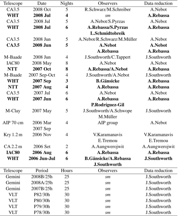
4.1 Overall observations of our project . . . 41

4.2 Log of the observations . . . 45

7.1 Radial velocities of 18 PCEBs and PCEB candidates, measured from the

Hαemission line and/or the NaIλλ8183.27,8194.81 absorption doublet. . . 63

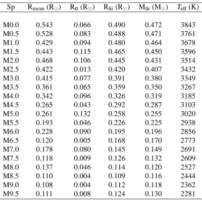
7.2 Empirical Sp−R, Sp−M and Sp−Teffrelations . . . 73

7.3 White dwarf masses, effective temperatures, surface gravities, spectral types

and distances of the SDSS PCEBs identified . . . 93

8.1 Radial velocities measured from the NaIλλ8183.27,8194.81 doublet . . . . 99

8.2 Orbital periods, semi-amplitudes Ksec, systemic velocitiesγsec, and reduced

χ2_{from sine fits to the Na}_I_{doublet radial velocity data . . . 103}

8.3 Average binary parameters obtained for seven PCEBs which have orbital

period and Ksecmeasurements. . . 107

8.4 Parameters of the PCEBs derived from calculating their post-CE evolution . 113

9.1 The complete catalogue of WDMS binaries and candidates. Near- and

far-ultraviolet, ugriz and yJHK GALEX, SDSS and UKIDSS magnitudes for

the 1591 WDMS binaries are also included . . . 133

9.2 The catalogue divided into different WDMS-type classes . . . 134

9.3 White dwarf masses, effective temperatures, surface gravities, spectral types

(10)

9.4 Radial velocities measured from the NaIλλ8183.27,8194.81 doublet and

the Hαemission of 1062 systems in our catalogue . . . 139

(11)

List of Figures

1.1 Roche-lobe equipotential surfaces . . . 5

1.2 Histograms of reconstructedγandαCEλvalues . . . 11

1.3 Current observed orbital period distribution of CVs . . . 14

1.4 Theoretical distributions of the secondary mass in present-day PCEBs, and Porbdistribution of the combined population of detached CVs and PCEBs . 17 2.1 White dwarf mass-radius relation . . . 22

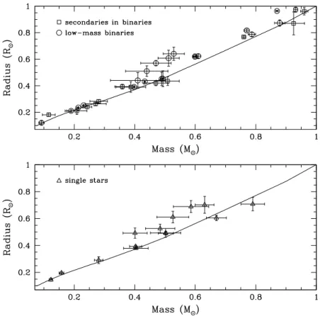
2.2 Observational mass-radius relation for low-mass MS stars . . . 26

3.1 Transition series of the atom of hydrogen . . . 29

3.2 Spectra of different white dwarf-type stars . . . 32

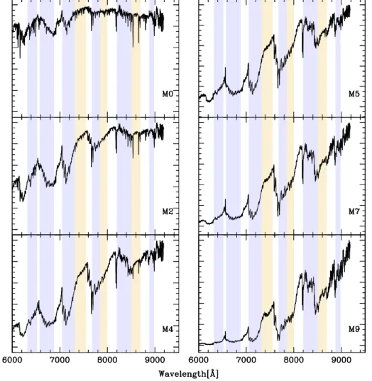
3.3 M-type star templates . . . 33

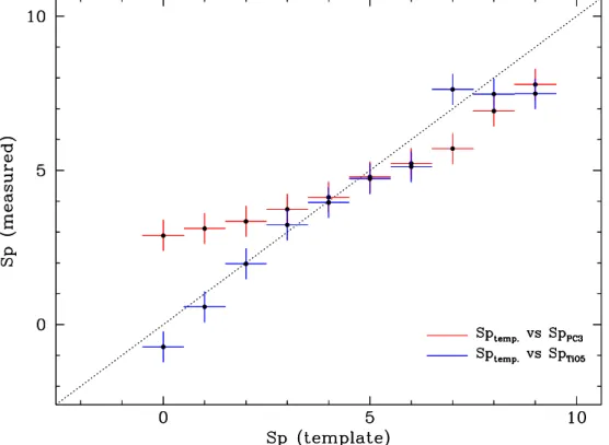
3.4 Comparison of spectral subtypes measured with different methods . . . 34

3.5 Three examples of SDSS WDMS binaries . . . 35

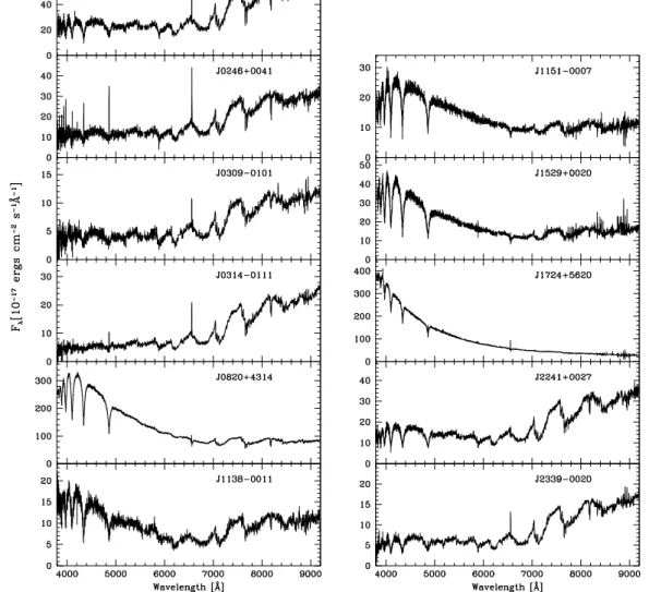
4.1 SDSS spectra of 11 WDMS binaries . . . 42

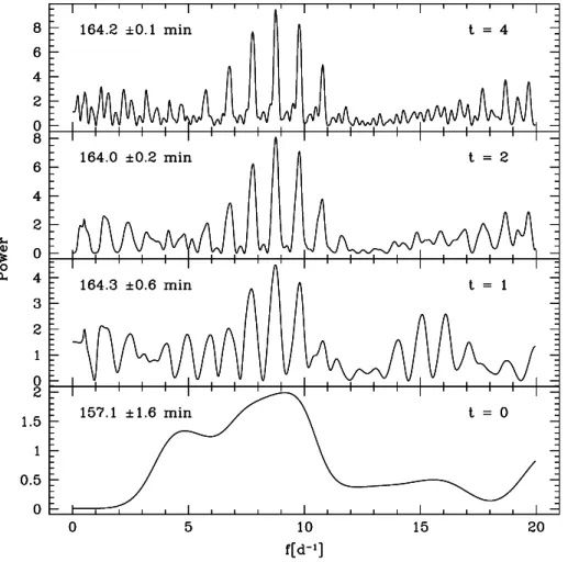
5.1 Power spectra of the PCEB SDSSJ 0052-0053 obtained along five consec-utive nights . . . 49

6.1 SDSS u,g,r,i and z filter responses . . . . 53

6.2 Northern and southern SDSS survey in galactic coordinates . . . 54

(12)

7.2 Radial velocities obtained from the NaIabsorption doublet . . . 61

7.3 Radial velocities obtained from the Hαemission line . . . 62

7.4 Two-component fits to the SDSS WDMS spectra . . . 68

7.5 Spectral model fits to the white dwarf component obtained after subtracting

the best-fit M-dwarf template . . . 69

7.6 Empirical Sp−R relation for M-dwarfs . . . . 72

7.7 Comparison of the white dwarf effective temperatures, distances and

spec-tral types of the secondaries determined from our fits and those of Raymond

et al. [2003] . . . 80

7.8 Comparison of the white dwarf effective temperatures and surface gravities

and the spectral types of the secondary stars determined from our fits and

those of Silvestri et al. [2006] . . . 81

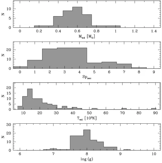
7.9 White dwarf mass, spectral types of the secondaries, effective temperature

and log g histograms . . . 83

7.10 Comparison of dsec and dwdobtained from our spectral decomposition and

white dwarf fits to the SDSS spectra . . . 88

7.11 Distances obtained using the Sp−R relation predicted by the models of

Baraffe et al. [1998], and adjusting the spectral type by 1–2 spectral subclasses 89

8.1 Scargle periodograms calculated from the radial velocity variations

mea-sured from the NaIabsorption doublet . . . 100

8.2 Radial velocity measurements folded over the orbital periods . . . 101

8.3 ORTperiodograms and light curves folded on strongest photometric

peri-odicities for SDSS J0314–0111 and SDSS J1724+5620, and the light curve

of SDSS J0820+4314 . . . 104

(13)

8.5 NaISDSS radial velocities along with the NaI radial velocities measured

in this thesis of SDSS J0309- 0101, SDSS J1138- 0011 and SDSS J2241+

0027. . . 112

8.6 The predicted evolution of two PCEBs . . . 116

8.7 Monte-Carlo simulations of the detection probability of significant radial velocity variations . . . 117

8.8 The period distribution of 41 PCEBs from the Ritter & Kolb [2003] (V7.9) catalogue containing a white dwarf plus M or K companion star . . . 118

9.1 Six WDMS binary templates . . . 122

9.2 χ2−S/N plane for two WDMS binary templates . . . 123

9.3 Two examples of recovered WDMS binary candidates that show blue and red excess, respectively . . . 125

9.4 SDSS images of three WDMS binary candidates . . . 127

9.5 (u−g,g−r), (g−r,r−i) and (r−i,i−z) colour-colour diagrams for the WDMS binaries in our sample . . . 131

9.6 Two-component fits to SDSSJ 0826+1941 . . . 137

9.7 Spectral model fit to the white dwarf component of SDSSJ 0826 +1941 . . 138

9.8 SDSS spectrum and near- and far-ultraviolet GALEX magnitudes of SDSSJ 0826 +1941 . . . 140

9.9 NaIdoublet radial velocities for nine close binaries . . . 141

9.10 Hαemission radial velocities for 16 close binaries . . . 141

9.11 Distributions of the stellar parameters for the systems in our catalogue . . . 144

9.12 Kolmogorov-Smirnov test for the distributions of stellar parameters pre-sented in Chapters 7 and 9 . . . 145

9.13 Comparison of dsecand dwdobtained from our spectral decomposition . . . 147

9.14 Density maps obtained from the stellar parameters . . . 149

10.1 Orbital period distribution of current SDSS PCEBs . . . 153

10.2 PCEB fraction among our observed WDMS sample . . . 156

(14)

10.4 PCEB and wide WDMS binary white dwarf mass cumulative distributions . 158

10.5 Comparison of the M−R relation for white dwarfs used in this thesis and

those provided in Panei et al. [2000] . . . 160

10.6 Fraction of active systems as a function of Galactic height . . . 162

10.7 Comparison of dsecand dwdmeasured for our observed systems . . . 163

10.8 Four WDMS binary colour-colour diagrams and colour-cuts . . . 165

(15)

Acknowledgments

I deeply thank Dr. Boris G¨ansicke for his excellent guidance through my PhD, for his

help and suggestions, and most importantly for making it possible for me to develop my

qualities as a researcher. I am also deeply thankful for his trust in me in this and other

projects. Without him this thesis would have been impossible.

I am greatly indebted to Prof. Tom Marsh for clarifying all kind of data reduction

problems, and specially I am deeply thankful for his patience at the beginning of my PhD.

I also thank him for providing his software.

I thank Dr. Pablo Rodr´ıguez-Gil for his help in my first individual observations, for

his suggestions and comments, and for sharing his vast observing experience. I thank Dr.

Matthias Schreiber for his trust in me as his future research assistant, and for clarifying

the-oretical problems I found during my thesis. I thank Dr. John Southworth for proof-reading

this thesis, and for his suggestions and comments. I thank Ada Nebot G ´omez-Mor´an for the

interesting discussions on binary evolution. I thank Dr. Linda Schmidtobreik for having me

as a visitor student at the European Southern Observatory in Chile. I thank Dr. Jorge Panei

for providing me his white dwarf mass-radius relation models. I thank Detlev Koester for

for providing his white dwarf model atmospheres. I thank Isabelle Baraffe for discussions

on the properties of low mass stars.

I deeply thank Yike for her love, for making me happy, for her support.

Finally thousand thanks to my parents. For being always present, even in the

(16)

Declarations

I declare that this thesis has not been submitted in any previous application for a higher

degree. Chapters 1-6 provide information gathered from the literature, except Chapter 4

(Sect.4.3), where I present observations carried out by myself and/or other collaborators. In

Chapters 7-9 I present my own work, and in Chapter 10 I use the results obtained throughout

this thesis and other observations that have not been published yet.

Chapter 7 is based on Rebassa-Mansergas et al. [2007]: A.Rebassa-Mansergas,

B.T.G¨ansicke, P.Rodr´ıguez-Gil, M.R. Schreiber, and D. Koester, ”Post-Common-Envelope

Binaries from SDSS. I: 101 white dwarf main-sequence binaries with multiple SDSS

spec-troscopy” MNRAS.382.1377R (2007).

Chapter 8 is based on Rebassa-Mansergas et al. [2008]: A. Rebassa-Mansergas, B.

T. Gänsicke, M.R. Schreiber, J. Southworth, A.D. Schwope, A. Nebot G ómez-Morán, A.

Aungwerojwit, P. Rodr´ıguez-Gil, V. Karamanavis, M. Krumpe, E. Tremou, R. Schwarz, A.

Staude and J. Vogel: ”Post-Common-Envelope Binaries from SDSS - III. Seven new orbital

periods” MNRAS.1.112 (2008)

Chapter 9 is based on: A. Rebassa-Mansergas, B. T. G¨ansicke, M.R., D. Koester and

P.Rodr´ıguez-Gil ”A catalogue of white dwarf-main sequence binaries from SDSS DR6”. To

(17)

Abstract

Close binaries containing a compact object make up a wide variety of objects. The

evolution of all close binaries depends crucially on the rate at which angular momentum is

extracted from the binary orbit. The two most important sources of angular momentum loss

are the common envelope phase and magnetic braking. Both processes have been known

for long but are still poorly understood, and significant progress will only be achieved if

they can be calibrated using innovative observational input. Post-common-envelope

bina-ries are probably among the best-suited class of objects to improve our understanding of

close binary evolution, because (1) they are both numerous and well-understood in terms

of their stellar components, and (2) they are not contaminated by the presence of an

accre-tion disc. The Sloan Digital Sky Survey provides the possibility of dramatically improving

the observational size of known post-common-envelope binaries, with already more than

1500 white dwarf-main sequence binaries having been identified. The major task is now

to identify those systems that have undergone a common envelope and to measure their

binary parameters. This new, large sample of well-studied post-common-envelope binaries

will then provide the much-needed constraints for further development of binary evolution

theory.

Through my PhD I dedicated all my efforts towards identifying

post-common-envelope binaries, obtaining orbital periods of these new systems, and determining their

stellar parameters. For this purpose, I adopted the following strategies:

(1) About 10% of the white dwarf-main sequence binaries in the Sloan Digital Sky

(18)

the NaIλλ8183.27,8194.81 absorption doublet and/or the Hαemission line in the

differ-ent spectra from each object, I was able to iddiffer-entify radial velocity variable stars, which

are prime candidates for being post-common-envelope binaries. This method resulted in

the identification of 18 new post-common-envelope binaries among 130 white dwarf-main

sequence binaries with multiple Sloan spectra. In addition, using a spectral

decomposi-tion/model atmosphere analysis I determined the stellar parameters such as mass, radius,

and temperature for the white dwarfs, and spectral types of the main sequence stars in

these 130 white dwarf-main sequence binaries, along with the distances to the systems.

I discussed also an apparent systematic issue with the spectral type-radius relation of the

companion stars in those white dwarf-main sequence binaries.

(2) Follow-up observations by our team have lead to the identification of 89

post-common-envelope binaries from Sloan, which triples the number previously known. Intense

radial velocity studies have lead to the determination of orbital periods for 42 of these

systems, seven of them discussed in detail in this thesis.

(3) I have developed a procedure based onχ2template fitting and signal-to-noise ratio constraints to identify white dwarf-main sequence binary candidates in the Sloan

Dig-ital Sky Survey Data Release 6 spectroscopic data base. This catalogue contains 1591 white

dwarf-main sequence binaries identified in this way. Using a spectral decomposition/model

atmosphere analysis, I have derived white dwarf temperatures, masses, companion star

spectral types, and distances, and discussed the distributions of these parameters. In

addi-tion, I have analysed the selection effects of white dwarf-main sequence binaries in Sloan.

This sample is an excellent data base for future follow-up observational studies of white

(19)

(20)

Chapter 1

Overview of Close Binary Evolution

1.1 Introduction

Most stars are formed as parts of binary or multiple systems1_{. Therefore the study of binary}

star evolution represents an important part of studying stellar evolution. While the majority

of wide main sequence (MS) binaries evolve as if they were single stars and never interact,

a small fraction are believed to undergo mass transfer interactions (Sect. 1.2.1). Once the

more massive MS star becomes a red giant it eventually overfills its Roche-lobe.

Dynam-ically unstable mass transfer exceeding the Eddington limit ensures onto the companion

star, which consequently also overfills its own Roche-lobe. The two stars then orbit inside

a common envelope (CE, Sect 1.2.2), and friction inside this envelope causes a rapid

de-crease of the binary separation. Orbital energy and angular momentum are extracted from

the binary orbit and lead to the ejection of the envelope, exposing a post-common-envelope

binary (PCEB). After the envelope is expelled, PCEBs keep on evolving towards shorter

orbital periods through angular momentum loss via gravitational radiation and, for

com-panion stars above the fully convective mass limit (≃0.3 MJ), by magnetic wind braking

(Sect. 1.3.1). In binaries that do not undergo a CE phase both components evolve almost

(21)

no mass transfer takes place, or when the mass transfer from the H-core burning donor star

(case A; this is the first epoch in which the leaving MS star undergoes a gentle growth of

its radius), from the He-core burning donor star (case B; in this case the expansion is more

rapid, towards the first giant branch), or from the post-He-core burning donor star (case

C; also rapid increase of radius, in this case the expansion is towards the asymptotic

gi-ant branch) to the MS companion is stable. A predicted consequence is hence a strongly

bi-modal binary separation and orbital period distribution among post-MS binaries, with

PCEBs concentrated at short orbital periods, and non-PCEBs at long orbital periods.

The scenario outlined above is thought to be a fundamental formation channel for

a wide range of astronomical objects such as double degenerate white dwarfs, cataclysmic

variables and super-soft X-ray sources. Some of these objects will eventually end their lives

as type Ia supernovae, which are of great importance for cosmological studies.

In the following sections of this Chapter, I give an overview of close binary

evolu-tion. In Sect. 1.2, I provide a description of the physical phenomena involved, and give

details of the CE phase. In Sect. 1.3, I deal with the evolution of PCEBs. Finally in

Sect 1.4, I describe the objectives of my thesis based on the theoretical background

de-tailed in Sect. 1.2 and Sect. 1.3. Throughout this thesis, I will use the term WDMS binary

to refer to the total class of white dwarf plus main sequence binaries, and PCEBs to those

WDMS binaries that underwent a CE phase. I also define a PCEB as a WDMS binary with

an upper limit to its orbital period ≤300 d, a PCEB candidate as a WDMS binary with

period 300 d≤Porb≤1500 d, following Fig. 10 from Willems & Kolb [2004], which shows

the period and mass distribution of the present-day WDMS binary population at the start of

the WDMS binary phase.

1.2 Formation of Post-Common-Envelope Binaries

Wide MS binaries are considered to be the progenitors of close compact binaries.

Popula-tion synthesis models predict that∼25% of the MS binary population suffer mass transfer

interactions [Willems & Kolb, 2004]. The stellar components of the remaining∼75%

(22)

are expected to undergo a CE phase and become close compact binaries, the details of their

evolution crucially depends on the conditions of mass transfer, and consequently on the

initial masses of both stars.

1.2.1 Mass Transfer

Roche geometry

Under the assumptions of Roche geometry (the orbits are circular, and the star that loses

mass, or donor star, is tidally locked), two orbiting stars have a total potential given by

the sum of the gravitational potential of the stars and the rotational potential of the system

(Eq. 1.1, whereωis the angular frequency of the orbit, r1 and r2 are the positions of the

two stars, M1 and M2 are the masses of the stars, being M1 the more massive component

at the initial MS binary configuration, and G is the gravitational constant). The shape and

dimension of the equipotential surfaces depend on the masses of the stars (or the mass ratio

q=M2/M1), and the orbital separation, respectively.

φ(~r) =− GM1 |~r−~r1|

− GM2 |~r−~r2|

−1

2(~ω×~r)

2 _(1.1)

The equipotential surfaces are mainly spherical for stars of small radius, and the shape is

distorted for larger radii. When the radii are sufficiently large the equipotential surfaces of

the stars cross each other (Lagrangian points). In Fig 1.1 I provide a schematic

represen-tation of Roche geometry for q=0.4. As seen in the figure, there exist five Lagrangian

points L1−L52. The two surfaces touching at L1, the inner Lagrangian point, are called

Roche-lobes. Mass transfer occurs when one of the stars overfills its Roche-lobe. If both

stars remain inside their Roche-lobes the system is detached. When one of the stars overfills

its Roche-lobe, mass transfer is then initiated towards the companion, and its shape is the

same as its Roche-lobe. The system is considered as semi-detached, and the Roche-lobe

radius of the donor star can be written as [Eggleton, 1983]:

RL=

a 0.49 q2/3

(23)

system is in contact. When this happens a CE is formed (Sect. 1.2.2), and matter can be

expelled through L2and L3.

Mass transfer in MS binaries

When the more massive component in a MS binary departs from the MS, its radius starts to

increase. The orbital separations of these binaries are normally wide enough for the Roche

equipotential surfaces to be spherical around each star, and to allow their evolution as if

they were single, i.e. no mass transfer interactions. Nevertheless, in∼25% of the cases the

evolved star is expected to overfill its Roche-lobe and mass transfer is then initiated to the

MS companion [de Kool & Ritter, 1993; Willems & Kolb, 2004]. The system’s response to

the mass loss can be extremely different depending on the initial masses of the stars.

If the donor is less massive than the accretor, and the thermal timescale3_{of the donor}

star is short enough to adjust the star to its equilibrium radius, the mass transfer will be then

dynamically and thermally stable. This can be understood considering the conservation of

the total angular momentum of the system: since the donor is less massive, the transferred

material ends up closer to centre of mass of the system, consequently losing angular

mo-mentum. In order to conserve the angular momentum of the system the binary separation

increases, so does the Roche-lobe radius (Eq. 1.2). Henceforth the donor star stops filling

its Roche-lobe, and mass transfer is stopped. The radius of the donor star though is

con-tinuously expanding, as it is evolving through the giant branch (GB), or asymptotic giant

branch (AGB), and consequently overfills its Roche-lobe again, leading to another process

of mass transfer, and to an additional increase of the Roche-lobe radius. This situation

re-mains until the donor leaves the GB, or AGB, and becomes a white dwarf. The resulting

system is then a wide WDMS binary, with a final orbital separation larger than the initial

MS binary separation.

If the donor star is more massive than its companion, the mass transfer will be

dynamically unstable. In this case the transferred material moves further from the centre

of mass, and the separation decreases in order to conserve the angular momentum. The

3_{Estimate of how long a given star would shine with its current luminosity if the only power source were the} conversion of gravitational potential to heat. The thermal timescale is also known as Kelvin-Helmholtz (KH) timescale, and can be written asτKH= 1₂

Egrav

L ≈ GM2

(24)

Figure 1.1: Cross section of Roche-lobe equipotential surfaces in the orbital plane of the semi-detached eclipsing binary BP Muscae, a binary with q = 0.4. The Lagrangian points are represented by L1-L5. The secondary star with mass M2 is overfilling its Roche-lobe,

and mass transfer results to the primary companion of mass M1. CM represents the centre

of mass of the system. The coordinates are given in RJ units. Taken from Carrier et al.

(25)

Roche-lobe radius decreases, and consequently the mass transfer rate increases

consider-ably. Under these circumstances the donor star can never readjust to its thermal equilibrium

radius, and consequently the mass transfer is also thermally unstable. The non-stopping

inflow of material on to the companion makes itself to be driven out of thermal equilibrium

and consequently it will fill its own Roche-lobe. Hence, the system initiates a contact phase,

referred to in the literature as the CE phase. The friction inside the envelope drives a rapid

(∼103 years) decrease of the binary separation through an in-spiralling process. The en-ergy and angular momentum extracted from the binary orbit ultimately eject the envelope

and give birth to a hot sub-dwarf/WDMS binary, surrounded by a planetary nebula. The

hot white dwarf cools down and the planetary nebula is dispersed, and the system is finally

observed as a PCEB.

The formation of a He- or a C/O- or O/Ne/Mg-core white dwarf depends on when

the mass transfer is initiated [Iben & Livio, 1993; Willems & Kolb, 2004]. If mass

trans-fer is initiated before the more massive star in the initial MS binary burns He into C, the

white dwarf will contain a He-core (MWD<∼0.5 MJ). If mass transfer initiates when a

substantial amount of He has been burnt into C/O, the resulting white dwarf will have a

C/O-core (0.5MJ<

∼MWD<∼1.1MJ). In the same way, if mass transfer starts when a

sub-stantial amount of C/O has been burnt into Ne/Mg, the resulting white dwarf will contain

an O/Ne/Mg-core (1.1MJ<

∼MWD<∼1.38MJ).

1.2.2 Common Envelope Phase

Qualitative description

Even though the concept of CE evolution is straightforward, it involves a large number of

hydrodynamic and thermodynamic processes on both time and scale lengths spanning very

large ranges. Moreover, it is intrinsically a three-dimensional problem.

Paczynski [1976] considered for the first time that the binary components move

inside a non-co-rotating envelope, transferring angular momentum and energy, and reducing

the orbital separation. The energy extracted from the orbit might be used to expel the

(26)

deposition of orbital energy into the envelope became evident. This efficiency is defined as

αCE=

∆Ebind

∆Eorb

(1.3)

where∆Eorb is the change in the orbital energy of the binary between the beginning and

the end of the spiral-in process, and∆Ebind is the binding energy of the ejected material.

Eq 1.3 neglects any other source of energy apart from the orbital energy. This comes from

the fact that CE evolution is rapid compared to the thermal time scale of the envelope, and

so radiative losses are small. Livio [1989] and Iben & Livio [1993] noted that, even though

αCE depends strictly on the orbital energy, the efficiency of deposition of energy into the

envelope could be modified by other physical processes. Two factors are believed to reduce

αCE: the efficiency in the energy transport [Taam et al., 1978; Meyer & Meyer-Hofmeister,

1979; Livio & Soker, 1984; Soker et al., 1984], and non-spherical effects [Bodenheimer &

Taam, 1984; Taam & Bodenheimer, 1989; Livio & Soker, 1988, see the definition ofβCEin

the next paragraph]. Among the physical processes that can increase the efficiencyαCE, the

recombination energy in the ionisation zones is the most plausible (i.e. the energy released

when the material of the envelope recombines is an extra energy that can be used to expel

the envelope). In fact, Han et al. [1994, 2002] include a second α-parameter in Eq 1.3,

characterising the fraction of the initial thermal energy content on the CE available for its

ejection. Nevertheless this has been strongly criticised by Soker & Harpaz [2003], since

(1) Eq 1.3 depends strictly on the orbital energy, and (2) an enhancement in mass-loss rate

provides final orbital distributions similar to those obtained including an extraα-parameter.

Livio & Soker [1988] not only considered the efficiencyαCE, but also defined two

more parameters: βCE and γCE. βCE parametrises the importance of three dimensional

effects, and is defined asτdecay/τkep, whereτdecay is the orbital decay timescale, and τkep

is the Keplerian timescale of the envelope. Thus whenβCE ≤ 1 no spherical symmetry

can be assumed, as the energy is deposited locally. γCE is defined asτspin−up/τdecay, where

τspin−up is the timescale for the spiralling-in binary to spin up the envelope, and describes

(27)

Theα-formalism

The change in gravitational energy∆Eorbin Eq. 1.3 can be written as

∆Eorb=

GM2Mc

2af

−GM2(Me+Mc)

2ai

, (1.4)

where Mcis the mass of the giant core, Meis the mass of the envelope, and Mgis the mass of

the giant (note that Meis approximately the mass lost by the giant and consequently Mc+Me

is approximately the mass of the giant Mg), M2is the mass of the companion, and ai and af

are the initial and final separations, respectively.

Several interpretations of the binding energy∆Ebindof the envelope and the binary

can be found in the literature [Tutukov & Yungelson, 1979; de Kool, 1990; Nelemans et al.,

2000; Nelemans & Tout, 2005]. Among them the most commonly used is [Nelemans &

Tout, 2005]:

∆Ebind=

G(Mc+Me)Me

λRg

, (1.5)

where Rg is the radius of the giant and λ is a parameter that depends exclusively on the

structure of the red giant. Dewi & Tauris [2000] found thatλnot only strongly depends on

the evolutionary stage, but also that λ∼0.2−0.84. λcan be approximated as [Webbink, 2008]

λ−1_∼₃_.₀₀₀₋₃_._816m

e+1.041m2e+0.067m3e+0.316m4e, (1.6)

where meis Me/Mg.

From equations Eq 1.3, Eq 1.4 and Eq 1.5 we obtain

GMgMe

Rgλ =αCE

GMcM2

2af

−GMgM2

2ai

(1.7)

This equation represents the outcome of the envelope as determined from the energy balance

between the binding and the orbital energies, referred in the literature as theα-formalism.

Values of αCE close to unity imply that the orbital decay is very efficient in expelling the

envelope. On the contrary, a lowαCEpermits the formation of shorter orbital period PCEB

systems, as the process is less efficient. Typical values of αCE are in the range∼0.15-1

[Bodenheimer & Taam, 1984; Taam & Bodenheimer, 1989, 1991; Livio & Soker, 1988; de

(28)

Kool, 1990; Terman et al., 1994; Maxted et al., 2006; Afs¸ar & Ibanoˇglu, 2008]. A plausible

value as low as 0.054 was found for V 471 Tau, an eclipsing DA+K PCEB [O’Brien et al.,

2001]. These results tell us thatαCEis far away from being a universal constant, and that it

probably depends on different binary parameters, such as the masses of the stars, the

evolu-tionary stage of the primary, and the nature of the secondary. Politano & Weiler [2007] have

initiated a comprehensive population synthesis study of variable CE efficiency parameters.

In this work (the first of the series) they assume both a power law dependence,αCE = M2n,

and a dependence in whichαCEapproaches 1 for large secondary masses andαCE= 0 below

some assumed cutoff mass,αCE=1−Mcut/M2, where Mcut is the cutoff mass. Politano &

Weiler [2007] find that the distribution of PCEB secondary star masses varies significantly

depending on the model used, and claim that a well-defined, statistically complete sample

of PCEBs would be desirable for a comparison with their population models.

Quantitative remarks of the Common Envelope phase

Although hydrodynamic studies have provided much insight into the phases of the CE stage,

calculations at high spatial resolution are still necessary to further quantify the outcome of

the envelope. As noted by Taam & Ricker [2006] and Ricker & Taam [2008] “in recent

years the development of sophisticated computer methodologies has made it possible to

achieve this goal. Specifically, adaptive mesh refinement techniques have advanced to the

point where such calculations can now be envisioned”.

Theγ-formalism

First Nelemans et al. [2000], and then Nelemans & Tout [2005] reconstructed the evolution

of observationally confirmed white dwarf binaries (double degenerates or DDs). A double

degenerate configuration is in principle achieved after two mass transfer processes, either

both being unstable (i.e. two CE phases), or the first being stable and the last unstable

(29)

the cores of giant stars from which they ascend. Thus the effect of the CE phase on the orbit

can be reconstructed. Nelemans et al. [2000], and Nelemans & Tout [2005] demonstrated

that the first phase of mass transfer can not generally be described by theα-formalism, as

they measured negative values ofαCEλ. This result was later confirmed by van der Sluys

et al. [2006] for the efficiencyαCE. Thus Nelemans et al. [2000] introduced a new algorithm

based explicitely on the equation for angular momentum balance

∆J J =γ

∆Mtot

Mtot

=γ Me Mg+M2

(1.8)

and found that thisγ-formalism could explain both phases of the evolution5. Unfortunately theγ-formalism still does not give a physical understanding of the process, and the results

are still open to debate [Webbink, 2008]. It is worth mentioning though that recently Beer

et al. [2007] proposed a physical mechanism that could explain theγ-formalism, based on

the accretion energy of some of the transferred matter. This energy could eject the remaining

matter and hence the systems could avoid the CE phase. Nevertheless, while comparing

their results with theα- andγ-formalisms, neither of them give a full description.

In Fig. 1.2 I provide distributions of reconstructed values of bothγandαCEλfrom

Nelemans & Tout [2005] derived from their analysis of the observed sample of DDs (top),

and observed pre-cataclysmic variables (bottom). Values of αCEλ cluster below ∼ 0.5,

implying that the orbital separations after the ejection of the envelope are considerably

lower than the initial separations. Consequently the energy equation does not work for

DDs because it predicts too short orbital periods. The angular momentum equation though

can explain all kinds of mass and Porb combinations with γvalues clustering in a small

range [Webbink, 2008]. As a consequence, the orbital periods for PCEBs will concentrate

to shorter orbital periods in theα-formalism than in theγ-formalism, and a longer tail to

longer orbital periods will be expected in theγ-formalism.

5_{Note that}_γ_{is not}_γ

(30)

0

1

2

0

1

2

3

4

0

2

4

6 γ

αλ

wd + wd

"pre-CV"

(31)

1.3 Evolution of Post-Common-Envelope Binaries

After the ejection of the envelope, PCEBs continue decreasing their orbital separations

(and orbital periods) through the action of angular momentum loss (AML) via the emission

of gravitational waves (referred in the literature as gravitational radiation, GR), and for

companion stars above the fully convective mass limit, and orbital periods short enough

for the secondary stars to be tidally locked (Porb <∼10 days), via the action of magnetic

wind braking [MB, magnetically-coupled stellar wind from the tidally locked companion,

Verbunt & Zwaan, 1981; Mestel & Spruit, 1987; Hameury et al., 1988]. Depending on the

nuclear time scale of the companion star (τnuc) and the AML timescale (τAML), the evolution

follows two different paths.

In general, PCEBs contain low-mass MS secondaries, and consequently τnuc ≫

τAMLin this kind of stars (see Chapter 2). SinceτAML(MB)∼108 years [Verbunt & Zwaan, 1981], this implies that the orbital separation shrinkage due to AML eventually makes the

secondary fill its Roche-lobe and a second phase of mass transfer ensues, in this case from

the low-mass companion to the white dwarf. If the mass transfer is thermally and

dy-namically stable, a cataclysmic variable is formed (see Sec. 1.3.1). If the mass transfer is

dynamically stable, but thermally unstable the system appears as a super-soft X-ray source.

If the mass transfer is dynamically and thermally unstable the system might enter a second

CE phase, which can lead to the coalescence of the two stars. This implies that the

sec-ondary star mass has to be significantly larger than the white dwarf mass. In these cases the

evolution is more likely to follow the description below.

In some cases PCEB companions are A-F stars, considerably more massive than the

above low-mass MS companions. These stars do not experience AML due to MB and

con-sequently they must wait for nuclear evolution to initiate mass transfer, i.e. they evolve into

red giants before mass transfer begins. The radius expands, the star overfills its Roche-lobe,

and mass transfer is initiated to the white dwarf. Since these stars are generally more

mas-sive than the white dwarf primaries, mass transfer is dynamically and thermally unstable,

and a second CE phase is likely initiated, which results in the formation of an

ultrashort-period DD. It is also possible, but not likely, that the mass transfer is both thermally and

(32)

day.

1.3.1 Evolution of cataclysmic variables

In the earlier 1970s it was already known that the orbital periods of cataclysmic variables

(CVs) are of order of hours, and that the material transferred from the Roche filling

secon-daries eventually forms an accretion disc [Paczy´nski, 1971]. Population synthesis studies

predict that 0.5-2% of the initial wide MS binary population become CVs [de Kool, 1992].

The time spent to become a CV after the ejection of the envelope is∼2 Gyr [Schreiber &

G¨ansicke, 2003].

The orbital period distribution of CVs (see Fig. 1.3) reveals three striking features:

(1) a long period cutoff at∼12 hours, (2) a short period cutoff at ∼80 minutes, (3) an

absence of systems between∼2−3 hours.

The long period cutoff is a consequence of dynamically stable mass transfer in CVs.

The absence of systems between∼2−3 hours, known as the period gap, can be

easily explained if AML due to MB somehow drops, and AML is driven out by GR. The

drop of MB can be associated with the transition of the secondary from a radiative core to

a fully convective state (Msec≃0.3 MJ, P

orb∼3 hours). This produces a reduction in the

mass transfer rate (from ˙M∼10−8−10−9MJyr−1above the gap to ˙M∼10−10−10−11

MJyr−1below the gap, where ˙M symbolises the mass transfer), and allows the secondary

to shrink towards its thermal equilibrium radius, causing a period of detachment [Rappaport

et al., 1983; Spruit & Ritter, 1983]. The CV remains detached until the star fills its

Roche-lobe again at Porb∼2 hours.

The minimum period cutoff occurs when the mass of the secondary star is so low

that it becomes degenerate. Mass loss in this kind of star produces an increase in radius,

and consequently the orbital orbital separation and orbital period of the CV increase also

(33)

Figure 1.3: Current observed orbital period distribution of CVs. The most striking features are the minimum period cutoff at∼80 minutes, the absence of systems between ∼2−3 hours, the period gap, and the long period cutoff at∼12 hours. The red solid line represents the cumulative distribution with numbers, N<Porb, as labelled on the right axis. Taken from

(34)

Disagreement with the observations

The standard evolutionary scenario of CVs provided above, together with the CE theory

presented in Sect 1.2.2 were used to develop population synthesis models for CVs. When

comparing these results with those obtained from observational studies, discrepancies arise.

Space densities obtained from population synthesis studies [ρ∼10−4−10−5pc−3de Kool, 1992; Kolb, 1993; Politano, 1996; Howell et al., 1997], are one order of magnitude larger

than those obtained from observational studies [ρ∼10−5−10−6pc−3,Downes et al., 1986; Ringwald, 1996; Schreiber & G¨ansicke, 2003; Pretorius et al., 2007; Ak et al., 2008]).

Pop-ulation synthesis models predict that∼99% of the intrinsic current CV population are below

the gap,∼70% of them are minimum period bouncers [Kolb, 1993], and that 18% of the

zero-age CV population contain brown-dwarf secondaries,∼80% of them formed as CVs

below the minimum period [Politano, 2004]. In contrast to this, an accumulation of systems

near the minimum period is not observed [Patterson, 1998, see though G¨ansicke et al. 2008,

in preparation], and similar numbers of systems can be found above and below the period

gap of the observed orbital period distribution (see Fig 1.3). The fact that the minimum

pe-riod calculated [∼70 minutes, Kolb & Baraffe, 1999; Barker & Kolb, 2003; Howell et al.,

2001] is shorter than the observed minimum period (∼80 minutes, Fig 1.3) exacerbates the

mismatch between the observed and calculated distributions. In fact different theories have

been proposed as an alternative to the standard scenario [Schenker et al., 2002; Andronov

et al., 2003; Taam & Spruit, 2001]. However, none of them have been successful in

match-ing all features found in the observed orbital period distribution, and the issue is still open

to debate.

1.4 Motivation and structure of the thesis

Close binary evolution has been mainly developed from the efforts carried out by theoretical

(35)

to test and calibrate the theory. Attempts to understand close binary evolution were initially

focused on the study of double cores inside a planetary nebula [de Kool, 1990; Livio, 1996].

These cores are the most direct evidence of a CE phase, and the study of their properties

are ideal to test the theoretical predictions, as a planetary nebula ensures that the observed

parameters are the same as those at the end of the CE phase. Unfortunately this kind of

system is very rare, as most PCEBs are very old and have undergone significant orbital

evo-lution after the CE [Hjellming & Taam, 1991]. Observational tests of the CE phase, based

on measurements of12C/13C and16O/17O ratios on the surface of the secondary star, were carried out by Sarna et al. [1995] and Marks & Sarna [1998]. However, results provided by

these studies were not conclusive [Dhillon et al., 2002].

Real progress in our understanding of close binary evolution is most likely to arise

from the analysis of PCEBs that are both numerous and well-understood in terms of their

stellar components – such as PCEBs containing a white dwarf and a MS star. Furthermore,

PCEBs are nearby and accessible with 2-8 meter telescopes, and they are not contaminated

by the presence of an accretion disc. Schreiber & G¨ansicke [2003] showed that the

sam-ple of well-studied PCEBs is not only small, but being drawn mainly from “blue” quasar

surveys, it is also heavily biased towards young systems with low-mass secondary stars –

clearly not representative of the intrinsic PCEB population, and can hence not be used for

comparison with population models [e.g. Willems & Kolb, 2004]. The Sloan Digital Sky

Survey (SDSS, Chapter 6) is currently dramatically increasing the number of known white

dwarf plus main sequence binaries, paving the way for large-scale observational PCEB

population studies (Chapter 9).

We have initiated an observational programme to identify the PCEBs among the

SDSS WDMS binaries, and to determine their binary parameters. Identifying all PCEBs

among the SDSS WDMS binaries, and determining their binary parameters is a significant

observational challenge. A large sample of PCEBs will answer three important questions

in close binary evolution: (1) The disrupted MB scenario predicts an increase of the

rela-tive numbers of PCEBs by a factor∼1.8 in the range of secondary spectral types M3-M5

[Politano & Weiler, 2006, see Fig. 1.4 left panel]. Assuming that MB is indeed disrupted,

(36)

Figure 1.4: Left: Theoretical distributions of the secondary mass in present-day PCEBs for four different assumed AML models: GR only (dotted line), GR+RMB (reduced MB, dashed line [Andronov et al., 2003]), GR+IMB (intermediate MB, dash-dotted line, [Ivanova & Taam, 2003]), and GR+DMB (solid line, disrupted MB or standard scenario). The y-axis has been arbitrarily normalised to facilitate comparison. Taken from Politano & Weiler [2006]. Right: orbital period distribution of the combined population of detached CVs and PCEBs for an initial mass ratio n(q) =1,αCE=0.6 (dashed line) andαCE=0.1

(dotted line). The peak apparent in all the distributions is due to the population of detached CVs, the PCEB orbital period distribution increases monotonically with Porb. Taken from

(37)

M4-M5. An additional test for the validity of MB is also discussed in Davis et al. [2008]:

assuming that MB is disrupted, the orbital period gap distribution of detached WDMS

bina-ries (considering as detached the combination of those WDMS binabina-ries with orbital periods

between 2-3 hours, and detached CVs crossing the period gap), shows a peculiar distribution

that can be observationally tested (see Fig. 1.4 right panel); (2) The strength of AML can be

estimated by comparing the orbital period distributions of PCEBs at different times of the

PCEB binary evolution; (3) Theα-formalism andγ-formalism differ in particular in the

pre-dicted orbital period distribution of long orbital period PCEBs (Sect. 1.2.2). Consequently,

identifying the long orbital period end of the PCEB population will clearly constrain current

theories of CE phase.

It is expected that a fraction of WDMS binaries will be eclipsing. Eclipsing binaries

are the key to determine accurate stellar masses and radii. Because short-period WDMS

binaries underwent CE evolution, they are expected to contain a large range of white dwarf

masses, which will be important to populate the empirical white dwarf mass-radius relation

(see Chapter 2). Eclipsing WDMS binaries will also be of key importance in filling in the

mass-radius relation of low-mass stars at masses<_∼0.4 MJ(see Chapter 2).

In this thesis I present preliminary results of our ongoing project dedicated to

iden-tify and measure orbital periods of PCEBs and the stellar parameters of both WDMS

bi-naries and PCEBs. The structure is as follows. In Chapter 2 I give details of the physical

properties of white dwarfs and low-mass MS stars. In Chapter 3 I give some insight into

the spectral properties of WDMS binaries. In Chapter 4 I provide a full description of the

observations carried out for the analysis presented in this thesis. In Chapter 5 I explain

the methods I used to measure the orbital periods of PCEBs. In Chapter 6 I provide a

de-scription of the Sloan Digital Sky Survey. In Chapters 7, 8 and 9 I present my results: in

Chapter 7 I make use of SDSS spectroscopic repeat observations to identify 18 PCEBs and

PCEB candidates from radial velocity variations. In Chapter 8 I present follow-up

spec-troscopy and photometry of 11 PCEB candidates identified in Chapter 7. In Chapter 9 I

present a catalogue of 1591 SDSS WDMS binaries. Finally, in Chapter 10 I discuss my

(38)

Chapter 2

Physical Properties of White Dwarfs

and M-type Stars

In this Chapter I give some insight into the physical properties of both white dwarfs and

M-type MS stars, and I point out how the study of WDMS binaries can help improving our

understanding of these kinds of stars.

2.1 White Dwarfs

2.1.1 Luminosity of a white dwarf

White dwarfs [see reviews by D’Antona & Mazzitelli, 1990; Koester, 2002; Hansen, 2004]

are the end product of stellar evolution for the vast majority of MS stars, with the exception

of the most massive stars. Contrary to normal MS stars, where the gravitational collapse is

prevented by the thermal pressure generated by nuclear energy, in white dwarfs this

con-traction is balanced by the pressure of the degenerate electrons. White dwarfs evolve in

time as they decrease their luminosity, a process referred to in the literature as the white

(39)

L(t)/LJ= (2.3×10−3)×M×t−7/5 (2.1)

At the stage of transition from progenitor to white dwarf the luminosity is given by

the energy generated by nuclear fusion in the core of the star. Nuclear fusion stops once the

star enters the white dwarf cooling track, and the luminosity of the white dwarf is given by

the thermal energy that the white dwarf possesses.

Energy transport

In the core of the white dwarf, the transport is dominated by the electron conduction, whilst

in the thin, non-degenerate envelope the transport is carried out by radiative and/or

convec-tive diffusion on a much slower time-scale.

2.1.2 Atmospheres

Sion et al. [1983] classified white dwarfs according to their stellar atmospheres. Thus DA

white dwarfs have H dominated atmospheres, and DB white dwarfs He dominated

atmo-spheres, the DA-type being the most dominant among white dwarfs. The reason why white

dwarfs are composed of pure H atmospheres is that the gravity is so strong that all heavier

elements sediment/sink down below the visible layers, i.e. the atmosphere. For moderately

warm (young) white dwarfs, the diffusion time scales of metals are only of the order of

days, so this happens very quickly [Koester & Wilken, 2006]. In the case of DB white

dwarfs (pure He atmospheres), the outer H layer has been completely lost, and He as the

next lightest element floats up to the top. There is no yet completely consistent

explana-tion for the DB white dwarfs [Wolff et al., 2002]. A small number of white dwarfs though

are composed of different elements in their atmospheres, such as C (DQ) and other heavy

elements (DZ). Hot white dwarf atmospheres composed of ionised He are called DO, and

cool stars which show no identifiable features, i.e. a continuous spectrum (see Chapter 3

for a definition of spectrum), are labelled as DC. Pre-white dwarf atmospheres are mainly

composed of He and/or a mixture of C, N and O, or H depending on the previous evolution

from the MS. The H-rich stars remain their whole lives as DA. He- and CNO-rich stars

(40)

to leave behind a surface of H as they cool. Thus at Teff∼30000 K there appear to be no He

dominated atmospheres (DB gap). Nevertheless, the convection zone develops as these

sys-tems cool, and consequently at Teff ∼30000−12000 K, 25% of these objects revert back to

DB-type. Below Teff ∼10000 K, the chemical evolution becomes more complicated, and

is not fully understood [Bergeron et al., 2001].

2.1.3 White dwarf mass distribution and mass-radius relation

It has been shown that the mass distribution of (DA) white dwarfs peaks sharply around

∼0.6 MJ [Koester et al., 1979; Bergeron et al., 1995a; Finley et al., 1997; Liebert et al.,

2005, see also Chapter 7 and Chapter 9]. White dwarf masses can in principle be measured

indirectly under the assumption of a mass-radius (M−R) relation [Chandrasekhar, 1935;

Hamada & Salpeter, 1961; Wood, 1995; Panei et al., 2000, 2007]. This implies knowledge

of the effective temperature and surface gravity of the white dwarf, that can be obtained

fitting the Balmer absorption lines (see Chapter 3 for a definition of Balmer lines, and

Chap-ter 7 and ChapChap-ter 9 for the application of the method), and/or knowledge of the gravitational

redshift, that can be measured if the systemic velocity of the white dwarf is known (e.g. in

a wide binary).

M−R relations make use of several assumptions regarding the composition of the

interior and the surface layers. However, it has to be stressed that the M−R relation has

not yet been observationally tested. In fact, the distribution of empirical masses and radii

shows a large scatter around the theoretical M−R relations [Schmidt, 1996; Reid, 1996;

Provencal et al., 1998, see Fig. 2.1]. Procedures in which no M−R relation for white dwarfs

(41)

Figure 2.1: White dwarf M−R relation. The black line represents the theoretical

Chan-drasekhar [1935] relation, the green, blue and red lines the He-core, C-core and Mg-core zero temperature M−R relations obtained by Hamada & Salpeter [1961]. Black solid

dots represent the M−R relation provided in Bergeron et al. [1995b] for Teff =

(5-10-20-40)×103K at a given mass (except for M = 0.2 MJ and M = 0.3 MJ, which show T

eff =

(5-10)×103K and Teff = (5-10-20)×103K, respectively). Dark gray solid dots are

(42)

2.2 M-type stars

2.2.1 Interior

M-type stars [see Chabrier & Baraffe, 2000; Chabrier et al., 2005] are the coolest among

the MS stars, with effective temperatures of less than∼3800 K (and higher than∼2200 K,

see Chapter 7), and also the most abundant in our Galaxy [Chabrier, 2003]. The mass in

this kind of star ranges from ∼0.5 to ∼0.1 MJ, and consequently the temperature in

the interior is low enough for the electrons to be partially degenerate (Tc∼106−107K).

Because of the low effective temperature M-type stars have convective cores and envelopes,

which grow in depth with decreasing temperature. When the convective envelope reaches

the convective core the star becomes fully convective.

MS stars find themselves in hydrostatic equilibrium, in which the thermal pressure

balances the gravitational force. In this stage of the evolution, the thermal pressure comes

from the burning of H into He in the core of the star, with the proton-proton (p-p) chain

being the burning mechanism at work in M-type stars. The rate at which stars burn H

determines the time spent in the MS. A direct consequence of this is that for p-p H burning

low-mass main sequence stars, the time spent on the MS is considerably larger than for

those stars which burn H through the CNO chain. This time can be estimated from the

following equation [Tuffs et al., 2004, see the appendix]:

tMS=4800

M MJ

−1/3

×107,M<0.4MJ (2.2)

tMS=1100

M MJ

−3

×107,0.4MJ≤M≤8.1MJ (2.3)

where the resulting tMSis in years. Thus M-type stars are not yet able to leave the MS, as

the time needed to do so is larger than the Hubble time.

Energy transport

(43)

convective, and consequently the total energy transport is given mainly by convective flux

in the entire star.

2.2.2 Atmospheres

Given the low temperature, most of the H and C in the atmospheres of low-mass MS stars

are locked into H2 and CO molecules, respectively. Excess O is bound to form molecules

such as TiO, VO, and H2O, with some amounts also of OH. Metal oxides and hydrides such

as FeH, CaH and MgH are also present (see Chapter 3 for further details).

2.2.3 Rotation-age-activity relations

Stellar magnetic fields are believed to be caused within the convective zone of stars. A

localised magnetic field exerts a force on the plasma, which rises to the photosphere and

creates starspots on the surface of the star. This phenomenon is referred to as stellar activity,

and the reaction of stars to stellar activity on their surface is known as spottedness. Due to

the differential rotation that the star undergoes, starspots inhibit convection and produce

zones of lower temperature.

Even though significant progress concerning the rotation-age-activity relations for

M stars has been made, more studies are needed to fully understand such relations. Given

the complexity of the issue, and the fact that this topic is not the central part of this thesis,

I summarise here the most important findings up to date: (1) old stars rotate slower than

young stars, i.e. the rotational period Prot increases in time [Kiraga & Stepien, 2007]; (2)

magnetic activity decreases with time [West et al., 2008]; (3) there is a strong increase in the

active lifetimes of stars in the spectral-type range from M3 to M5 [West et al., 2008]; (4) fast

rotation excites magnetic activity up to a saturation threshold of vrotsin i∼10 km s−1, where

vrot is the rotational velocity, and i is the rotation axis inclination of the star2. Nevertheless

rotation and activity are not always linked [West & Basri, 2008, see also Chapter 10], (5)

activity-Prot relations found for young stars are not modified below Sp = M3.5-4, where

stars are supposed to become fully convective [Delfosse et al., 1998], (6) Prot decreases

linearly with increasing mass at a given age [Cardini & Cassatella, 2007], (7) M stars in

(44)

close binaries rotate faster than single M stars, or M stars in wider binaries [Cardini &

Cassatella, 2007].

2.2.4 Theory versus observations

Studies have been developed to create evolutionary stellar models, and to derive

theoreti-cal relations between the physitheoreti-cal parameters of low-mass MS stars [Baraffe & Chabrier,

1996; Baraffe et al., 1998, 2002, 2003]. However, when comparing empirical results with

the theoretical expectations numerous discrepancies arise [Ribas, 2006; Ribas et al., 2008].

Thus for example, current models predict radii that are∼15% smaller than the observed

values, and effective temperatures that are∼5% higher for star masses above∼0.3 M⊙

(see Fig. 2.2). Problems are thought to arise due to the high magnetic activity level that

a large number of this kind of star display, which is likely to affect the M−R relation

[L ´opez-Morales, 2007; Chabrier et al., 2007; Morales et al., 2008]. Moreover, the

proper-ties of low-mass stars are expected to change depending on their metalliciproper-ties [Berger et al.,

2006]. The spectral type-radius relation for M stars is also extremely affected by these

features (see Chapter 7). Below∼0.3 M⊙ there is a good agreement between the

observa-tional measurements and the models (Fig. 2.2). Nevertheless, this result can be misleading,

since “all objects in this range have rotational velocities vrotsin i<10 km s−1” [L

´opez-Morales, 2007]. Consequently more radius measurements of active stars in this range are

still necessary to confirm the apparent good agreement between the theoretical values and

(45)

Figure 2.2: Observational M−R relation for stars below 1 MJ. Top: empirical values

from low-mass secondaries to eclipsing binaries with primaries more massive than 1 MJ

(squares) and the components of eclipsing binaries below 1 MJ (circles). Bottom: all the

(46)

Chapter 3

Spectral Properties of White

Dwarf-Main Sequence Binaries

In the previous Chapter I have discussed in some detail the physical properties of both white

dwarfs and M-type MS stars. In this Chapter I will focus on the spectral features observed

in these kinds of stars, and also on the spectral properties of WDMS binaries. For this it

becomes necessary first to introduce spectroscopy as a technique in astrophysics, and to

understand what a spectrum is and how it is formed.

3.1 Spectroscopy

Spectroscopy gave birth to astrophysics as an observational science in the 1860s. This

tech-nique measures the flux emitted by an object in a certain wavelength (λ) range, providing

consequently a unique flux-wavelength dependence for each celestial object. Spectroscopy

implies the use of a spectrograph, which consists normally of a slit, a collimator, and a

dispersive element, such as a grating. The slit is situated on the focal plane of the telescope,

and isolates the light that comes from the target from other objects in the field. The light

(47)

dis-uum. These spectral features can appear in absorption or emission depending on the

tem-perature gradient in the atmosphere1. Let’s consider as an example the stellar atmosphere of a single star. The crucial parameter in the formation of the spectral lines is in this case

the optical depth

τν= Z

χνdz (3.1)

whereνis the frequency (or wavelength, since ν=c/λ) considered, χ_ν is the absorption coefficient of the atmosphere at a given frequency, and z the geometric depth. A stellar

atmosphere is optically thick when τ_ν>1, and optically thin when τ_ν<1. An optically

thick atmosphere emits practically like a blackbody2

I_ν∼B_ν (3.2)

where I_ν is the intensity emitted by the atmosphere and B_ν is the intensity emitted by a

blackbody. The energy emitted in an optically thin atmosphere is given approximately by

I_ν∼I_ν(τ_ν) +B_ντ_ν (3.3)

where I_ν(τ_ν)is the intensity emitted in the optically thick atmosphere layer

immedi-ately interior to the optically thin atmosphere. Spectral lines in a spectrum are formed when

the optically thin atmosphere of the star becomes optically thick due to increases of the

absorption coefficient. In this context, and depending on the temperature gradient between

the thin and the thick atmospheres, the line will be in emission or in absorption. If I_ν(τ_ν)

= 0, then B_νwill always be larger than B_ντ_ν and hence an emission line will always form.

Assuming that I_ν(τ_ν)is positive, then an emission line will form if B_ν>I_ν(τ_ν) +B_ντ_ν. In this case the inner layers of the atmosphere must be cooler than the outer layers, and the

temperature gradient then points to the surface of the star. When the inner layers are hotter,

the temperature gradient points the core of the star and B_ν<I_ν(τ_ν) +B_ντ_ν. In this case an absorption line is formed.

The crucial question is then why the absorption coefficient increases at a given

frequency. The physics of stellar atmospheres tells us thatχν is strongly dependent on the

population of electrons on a certain level l in a considered atom, and on the probability of

(48)

Figure 3.1: Three transition series of the atom of H. Transitions between the ground level and higher elements form the Lyman lines (e.g. Lyα, transition between levels 1 and 2), transitions between level 2 and higher levels form the Balmer lines (e.g. Hα, transition be-tween levels 2 and 3), transitions bebe-tween the third level and higher levels form the Paschen lines.

exciting an electron from the level l to another level u, flu. In a stellar atmosphere photons

and atoms are continuously interacting, and consequently the probability of exciting an

electron due to the absorption of a photon by an atom increases dramatically. After a certain

time the electron is de-excited and liberates a photon which can be absorbed by another

atom. These processes are called bound-bound interactions. Thus, if the atomic level is

sufficiently populated, and the probability of exciting an electron is high, the absorption

coefficient can be dramatically increased. Since the transition of the electrons are given