Implementing a real time control algorithm of Triana on SASensor Open Platform

on SASensor Open Platform

Prof.dr.ir. Gerard J.M. Smit, Dr.ir. Vincent Bakker, Gerwin Hoogsteen,

Dr.ir. Omar Mansour, Prof.dr. Johann L. Hurink

Qiang Fu

Abstract

In terms of electricity generation, Distributed Generation (DG) using Photovoltaics (PV) panels has become more common. To deal with the potential challenges it brought on the existing electricity distribution network, Demand Side Management (DSM) methodologies are developed. Triana, developed by Computer Architecture and Embedded Systems group (CAES) of University of Twente, is one of them. It is divided into three steps. In the first two control steps, it is able to utilize simulation or measurement data off-line to forecast and plan electricity production/ consumption on the device level.

Since prediction and planning errors can be caused by fortuitous behaviors of end users, it is often impossible to foresee it and prevent it from happening. It is however possible to detect these errors and solve them using a real-time control algorithm in the third step of Triana. The design, implementation and testing of this real-time control algorithm are included in this thesis.

In cooperation with Locamation, an Application Programming Interface (API) is added to the Triana to detect prediction and planning errors. Power, voltage and current data of medium voltage (MV) to low voltage (LV) transformers can be gathered in real time from the SASensor open platform. From the SASensor open platform, Triana can access the real-time measurement data (RTD) to detect overloading problems, deviation from original plan, etc.

Upon detection of intolerable prediction/ planning errors, the real-time control algorithm tries to perform replanning based on the deviation (measured in real-time) from its original plan. This new plan aims to quickly compensate for this deviation, preferably without violating other requirements (such as electric vehicle (EV) charging deadlines).

Acknowledgments

Upon completion of my master thesis, firstly I want to thank my family for their unconditionally support throughout the last two years. Without their assistance I could not imagine finishing my master’s study in a foreign land so far away from home.

During the last seven months at CAES and Locamation, I never cease to be amazed by the excellent academic achievements, professional work attitude and persistent pursuit of knowledge of all their members. Especially I am greatful to my supervisors, Prof.dr.ir. Gerard J.M. Smit, Gerwin Hoogsteen, Dr.ir. Omar Mansour, Dr.ir. Vincent Bakker and Prof.dr. Johann L. Hurink. Their guidance and generous help throughout the last seven months inspired me.

I also appreciate each course I took at University of Twente. The sparkling intelligence of all the teachers made all of them great enjoyment.

Contents

Abstract i

Acknowledgments iii

1 Introduction 1

1.1 Motivation . . . 1

1.2 Task statement . . . 2

1.3 Research questions . . . 4

1.4 Approach . . . 8

1.5 Outline . . . 8

2 Background and Related Work 9 2.1 The source of measurement data . . . 9

2.1.1 SASensor Open Platform . . . 9

2.1.2 Kernel-based Virtual Machine (KVM) . . . 11

2.1.3 Nahanni . . . 11

2.1.4 Application . . . 12

2.2 Triana . . . 13

2.2.1 Triana approach in theory . . . 13

2.2.2 Work flow of existing Triana simulator . . . 14

2.2.3 Power peak shaving . . . 15

2.3 Network modeling . . . 18

2.3.1 Lochem . . . 18

2.3.2 Load-flow simulation . . . 20

3 Design Decisions and Real-time Control Algorithm 21 3.1 Design decisions . . . 21

3.1.1 Strategy explorations . . . 21

3.1.2 How to replan the controllable loads to keepPplan0(t) as close to P_plan(t) as possible . 24 3.1.3 Necessary measurement data . . . 28

3.1.4 Scheduling memory access . . . 29

3.2 Real-time control algorithm . . . 29

4 Simulation Results and Analysis 31 4.1 Use case . . . 31

4.2 Results and analysis . . . 33

4.2.1 Case 1: uncontrollable load is lower than predicted . . . 33

4.2.2 Case 2: uncontrollable load is higher than predicted . . . 36

4.2.3 Case 3: EV leaves earlier than predicted . . . 39

4.2.4 Case 4: EV arrives later than predicted . . . 41

4.2.5 Case 5: Uncontrollable load shifts over time . . . 43

4.3 Conclusion . . . 46

5 Conclusion and Future Work 49 5.1 Future work . . . 50

1

Introduction

1.1

Motivation

Energy has always been one of the driving forces promoting the advance of human society. In modern society, electricity plays an important role powering not only factories but also households. Traditionally, electricity has been produced centrally in large plants. It was transported through the high voltage (HV) grid down to the LV distribution network [9]. However, a trend in the coming decades shows that a larger part of electricity demand will be generated in distributed setting [2]. PV panels, wind turbines and micro-Combined Heat and Power (µCHP) emerge as distributed power generators, which are even possible to be installed in households. This new trend caters to the increasing demand of electric energy. But at the same time, it brings challenges. One of them is that since the old distribution network is not designed with DG like this in mind, the extra load may put the existing network in danger. Thus an improved version of the grid calledsmart grid is introduced . A definition of smart grid is given in [18]:

Definition 1.1 A Smart Grid generates and distributes electricity more effectively, economically, securely, and sustainably. It integrates innovative tools and technologies, products and services, from generation, transmission and distribution all the way to customer devices and equipment using advanced sensing, communication, and control technologies. It enables a two-way exchange with customers, providing greater information and choice, power export capability, demand participation and enhanced energy efficiency.

Smart grid technologies can be divided into three categories [2]: DG, Distributed Storage (DS) and DSM). Among them, research focusing on DSM technology has been conducted within CAES of the University of Twente for the last few years [2] [10] [14].

Definition 1.2 DSM is the planning, implementation, and monitoring of utility activities designed to influence customer use of electricity in ways that will produce desired changes in the utility’s load shape, i.e., changes in the time pattern and magnitude of a utility’s load. [4]

Triana is a three-step DSM control methodology developed within CAES for smart grids. With

information from households and LV grids, it can be used to flatten the energy profile and improve power quality. In the first two control steps, it is able to utilize simulation or measurement data off-line to forecast and plan electricity production/ consumption on the device level. In the third step, a real-time control algorithm is applied to control each device at every time interval, ensuring the achievement of the plan. Triana simulator is an application developed within the CAES to realize this three-step control methodology. At the moment it supports simulation data and measurement data input.

However, sometimes when DSM methodology is applied, LV grid can still be subject to all kinds of problems. For example, DSM methodology aiming at reducing the overall energy bill may tend to converge controllable loads to low-price time. Whereas at the same time if uncontrollable loads behave unexpectedly from prediction, the overall power profile will deviate from its original plan. In an extreme case the LV grid might be overloaded. This overloading problem can lead to peak power demand and voltage drop, wearing the cables and bringing security problems.

To detect prediction and planning errors, power, voltage and current data of MV to LV transformers must be gathered in real time to be analyzed. At the moment, these data cannot be accessed and made use of in Triana yet. Thus making them accessible for Triana is targeted as another goal of this thesis.

To tackle this problem, this master thesis assignment is carried out within the CAES of the University of Twente in cooperation with Locamation. Locamation is a Dutch company which develops automation solutions for the smart grid. SASensor [1] [16], a substation automation platform within the MV and LV substations, is one of its products. It can continuously measure and monitor the electricity flow within the substation/transformers, making it a suitable choice for the source of RTD.

Now all measurements are available within ARTOS, a real-time operating system (OS) developed by Locamation. To allow customers of Locamation to utilize all those RTD, open platform V2 emerges. Avoiding running third party applications directly on ARTOS, it explores the possibilities to establish communications between applications running in parallel in different OSes. To be specific, by making use of KVM [6] [7] [11] [17], multiple guest OSes can be created and hosted by a Linux host. And one of the guest OSes is ARTOS, measuring and providing RTD available for third party applications running on host Linux or other guest OSes. Thus the remaining question is how to make RTD on ARTOS accessible for those applications, to be specific, for the Triana simulator in our case.

Under the premise of using KVM as the hypervisor, several inter-virtual machine (VM) data

communication techniques can be exploited. Among them, a communication mechanism based on POSIX shared memory called Nahanni [12] was chosen by Locamation. It is free to be used commercially and it allows user-level data transmission between applications. Since Locamation is responsible to provide RTD from the ARTOS side for applications running in Linux to access, this thesis will mainly focus on Linux side running Triana simulator. For performance reasons, the Triana simulator is chosen to run on host Linux. Coupling ARTOS with the Triana simulator, the designed SASensor Open Platform V2 architecture is shown in Figure 1.1.

1.2

Task statement

To summarize, the main goal of this master assignment is to design a real-time control algorithm to determine and solve prediction and planning errors. It is the major objective of the designed system. Furthermore, an API must be added to the Triana simulator to access data residing in the shared memory as well. To be precise, upon detection of prediction and planning errors, the real-time control algorithm must react properly so that the following criteria are met.

ˆ Upon detection, it must be ensured that overloading problem will be solved as soon as possible.

ˆ The overall power profile remains as close to its original plan as possible.

ˆ Charging deadlines of EVs set by end users are not violated.

Once necessary choice must be made among conflicting criteria based upon their priorities.

To prove the validity of the designed API and real-time control algorithm, the original plan is to apply it into the field test. For this purpose, the Lochem project is chosen.

Figure 1.1: Designed SASensor Open Platform V2 architecture

the impact of high penetration of PV panels and EVs within LV grid. Furthermore, as discussed in [8], in two stress tests that have already been conducted there, large amount of EVs charing at the same time overloaded the LV grid, showing great impact on power quality. Because of those reasons, Lochem is considered a suitable test site for the real-time control algorithm.

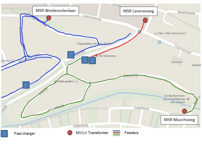
The site of the first stress test in Lochem is shown in Figure 1.2. All three transformers and four feeders are metered and the power consumption of 83 households is known, among which 33 provide the Root Mean Square (RMS) voltage magnitude measurements.

However, due to time constraints the designed API and real-time control algorithm can not be tested in the field test. But since the Triana model of Lochem project is available, it is still possible to test if this additional functionality works as expected in simulation environment.

In the field test, the RTD are measured by sensors and sent to ARTOS. Hence in simulation a reliable substitute source of RTD must be found so that the control loop can be closed. The load-flow simulator discussed in section 2.3.2 provides a work around this issue as can be seen in Figure 1.3.

Figure 1.2: Test site in Lochem

Figure 1.3: The control loop to test API and real-time control algorithm in simulation

However, to use the Triana model of Lochem project and the load-flow simulation as substitutions, their correctness must be ensured. In [8], they are verified using the information of the stress test conducted in Lochem. With the power profile of one of the feeders, the Triana network model and the location and measurement data of all fast charging poles, under several assumptions, the load-flow simulation shows the similar trend and voltage drop as measured in one of the meters, as shown in Figure 1.4 [8].

Some system errors might be included in the algorithm to perform load-flow calculations. Furthermore, the network model does not incorporate the effects of temperature, depth and surface type [8]. In addition, not all measurement data and location of households are available so assumptions and compromises must be made. However, from the observations of Figure 1.4, it is clear that despite all those errors, the Triana network model of Lochem project and the load-flow simulation can be trusted alternatives to test the designed API and real-time control algorithm in simulation.

1.3

Research questions

Figure 1.4: Voltage drop in the simulation and measured in one of the meters, taken from [8]

devices in real life can correctly execute their planned power profile, via controlling the functional states of those devices the real-time control algorithm can influence power more than other two factors. Thus it is reasonable to use it as the starting point while exploring the real-time control algorithm.

LetPtotal(t) be the overall power consumption at timet, at any state it can be divided into controllable

partPcontrol(t) (consumed by controllable devices), uncontrollable partPno control(t) (consumed by

uncontrollable devices) and unknown partPunknown(t) (consumed by the cables, etc.),

Ptotal(t) =Pno control(t) +Pcontrol(t) +Punknown(t) (1.1)

However since the duration of the simulation is set to one day which is way longer than that of the stress test, measurement data of the stress test can not be imported as the profile of the households

(uncontrollable). Therefore there is no sufficient data to perform load-flow simulation. To work around this issue, in the simulation the profile generator developed by G.Hoogsteen (one of my supervisors) was in use. As a result, the load-flow simulator is excluded from the simulation and the control loop is simplified into what is shown in Figure 1.5.

Figure 1.5: Simplified control loop to test API and real-time control algorithm in simulation

Since the profile generator can only generatePno control, Equation 1.1 is simplified into Equation 1.2.

difference betweenPunknown in simulation and that in field test no longer exists.

Ptotal(t) =Pno control(t) +Pcontrol(t) (1.2)

Since in our use case, devices within households in Lochem cannot be steered (i.e. uncontrollable), EV fast charging pole(s) are the only subject(s) which can be controlled. Suppose there areN charging jobs in total,Pcontrol(t) is then equal to the total power consumption of all EV charging job(s) at all time.

Pcontrol(t) = N

X

i=1

Pev(i)(t) (1.3)

wherePev(i)(t) represents the charging power of thei−thEV charging job at timet.

LetPplan(t) represent the overall power plan at timet. Based on equation 1.2 and 1.3, it can be

concluded that whenPtotal(t) deviates fromPplan(t), the reason might be wrong prediction of

uncontrollable powerPno control(t) or unreachable plan of EV charging job(s) Pev(i)(t). At timet, this

deviationPdev(t) can be represented by,

Pdev(t) =|Ptotal(t)−Pplan(t)| (1.4)

WhenPdev(t) exceeds the preset margin, actions must be taken to correctPplan(t) in the future. Since the

only control subjects are EV charging jobs, one or even all of them must be rescheduled so that the new overall planPplan0(t) can approximate the original planP_plan(t) in the future.

In previous work, the modeling of LV network and household appliances, the prediction and planning of the Triana approach are well studied, implemented and tested. Therefore to reuse part of the original code base and algorithms of the Triana simulator can simplify the work of this thesis and improve its reliability. Some functionalities/ features might be reused are listed as follows.

ˆ The planning algorithm of EV discussed in [5] and [24].

ˆ The Triana network model of the test site of Lochem.

Because the planning algorithm and code of single EV is given, this thesis will focus on how to distribute

Pdev(t) to controllable loads so thatPplan0(t) can remain as close to the original overall planP_plan(t) as possible.

Suppose a simple scenario with single household and three fast charging poles as shown in Figure 1.6. As in the Lochem case only the fast charging poles are controllable. WhenPdev(t) exceeds the preset margin,

there are several possible reasons,

ˆ Pno control is lower than its predicted valuePno control pre. In this case, the charging power of available

EV(s) can be increased such that the difference betweenPplan(t) andPtotal(t) is compensated.

ˆ Pno control is greater than its predicted valuePno control pre. Compared with the previous occasion,

this one may cause the delay of EV charging jobs since in this occasion to stick to the original plan

Pplan(t), EV charging job(s) must decrease its charging power. It is also necessary to make a replan

whenPno control(t) drops back to or below its predicted value so that the charging deadlines set by

end users can be met.

Figure 1.6: A simple example matching the scenario in Lochem

ˆ Early leave time of EVs. In this case, Ptotal(t)≤Pplan(t). It is similar to the first scenario of

prediction errors and the same strategy may also work in this case.

ˆ Late arrival time of EVs. In this case, other available EV charging jobs can be replaned to make up forPdev(t) and when the new EV arrives, it can still meet its deadline utilizing the power ”saved” by

other early charging EVs.

Although there are more complicated scenarios, they can normally be solved by using the strategy of one of the cases mentioned above. For example, when overloading problem happens, the strategy used when

Pno control is greater than its predicted valuePno control pre can be adopted. A more realistic case is when

uncontrollable power peak shifts over time, which can be treated as the combination of the first two aforementioned scenarios.

In the aforementioned four simple scenarios, common challenges faced are which strategy to choose while performing the real-time control algorithm and how to make a replan for relevant EV charging jobs. Therefore my research question for the real-time control algorithm is,

ˆ How to design the real-time control algorithm incorporated into the Triana simulator to realize the aforementioned objective of the system?

– Which strategies to choose while performing the real-time control algorithm?

– How to replan the controllable loads to keep Pplan0(t) as close toP_plan(t) as possible?

Also for the real-time control algorithm to access RTD, two major decisions must be made to design the RTD API. Each one of them forms a sub research question. Only by answering all of them can the best design of RTD API be found. For this part, my research question is:

ˆ What is the best design for the API of the Triana simulator to access RTD?

– Based on Nahanni shared memory, what is the most efficient way to schedule shared memory access? (polling, interrupt, etc.)

1.4

Approach

The code base of the existing Triana simulator must be studied.

ˆ To maximize reusability, information must be extracted from the model of EVs and the planning algorithm of Triana to determine which strategy is most suitable.

ˆ It is necessary to figure out how to steer the selected device to make a proper replan for them.

In addition, a literature study will be conducted to answer the sub-questions listed above.

ˆ Literature study can provide ample information about the data needed to detect prediction/ planning errors. This depends on the use case.

ˆ To find the most efficient way to schedule memory access, polling, interrupt and other approaches must be compared as well. Pros and cons of each approach is available in literature.

1.5

Outline

2

Background and Related Work

Section 2.1 describes the source of RTD. How RTD is measured, put in ARTOS and then made available for the Triana simulator is included in this part. SASensor Open Platform V2 (section 2.1.1) enables communication between VMs via Nahanni shared memory (section 2.1.3) provided KVM (section 2.1.2) is utilized.

Followed is the description of Triana, both theoretical and practical. A brief introduction of how Triana approach is devised initially in theory is given at first. It is one of the theoretical background of the thesis. Then how the Triana approach is implemented as the newest simulator is described. It is essential to understand how it works to make modifications to it. A brief introduction of the concept of power peak shaving and how it is realized in the planning algorithm of Triana is described later. Flattening the power profile is one of the most important objectives of Triana.

Remaining topics are network modeling. Lochem project and its Triana network modeling are introduced. It is the use case of this thesis. At last, the additional module of the Triana approach, load-flow simulator is introduced briefly.

2.1

The source of measurement data

2.1.1 SASensor Open Platform

SASensor, as described before, is a substation automation system which is capable of performing various substation automation tasks. It can be further divided into SASensor High Voltage, SASensor High Medium Voltage (HMV) and SASensor Medium Voltage (MLV). For the remainder of this thesis, SASensor will refer to SASensor MLV platform installed within substation end.

A basic SASensor architecture can be composed of components listed below.

ˆ Interface Modules, which can be subdivided into three types.

– Current Interface Module (CIM), connected to current transformer for current measurements. – Voltage Interface Module (VIM), connected to voltage transformer to measure voltage. – Break Interface Module (BIM), which can sense the position of switch gears and actuate them

when necessary. [1]

ˆ Central Control Unit (CCU), which is capable of performing complex computations and controlling the behavior of BIMs.

ˆ Versatile Communication Unit (VCU), connected to both the platform and remote control center, is responsible for remote operations and maintenances as well as substation information access. Figure 2.1 shows all units mentioned above as well as their connections in a SASensor architecture example.

Figure 2.1: An example of SASensor architecture, taken from [16]

Currently the whole ARTOS is accessible via a web-based graphical user interface (GUI) which allows its user to navigate its file system hierarchically. However, efforts have been made to make SASensor an open platform for third party applications. The definition of Open Platform is given in [13],

Definition 2.1 An Open platform is a SASensor automation system where clients (non-Locamation or 3rd party developers) can design and configure their substation and implement new ideas and functionalities in a non-proprietary manner.

In SASensor Open Platform V1, several attempts are made to simplify the substation engineering process and reduce the dependency on the special expertise of Locamation’s engineers. In [16], several ideas are initiated including developing new applications directly in C, translating Matlab/Scilab specifications to C, etc. However, all of them seem to bring platform-related restrictions and require certain knowledge of ARTOS. In [1], the notion of application store introduces a complex procedure of application development to protect (3rd party) Intellectual Property and ensure authority and role rules are enforced. But it still fails to solve problems aforementioned completely. However, getting rid of running third party applications on ARTOS, SASensor Open Platform V2 is a possible solution.

The concept of SASensor open platform V2 aims at providing better security, system reliability and richer set of tools for the 3rd party developers [13]. SASensor open platform V2 takes advantage of KVM by running ARTOS as one of its guest systems. Guest-guest and host-guest communications ensure the availability of RTD. Therefore, third party applications can run on its designed platform without compromise. In the following sections, the notion of KVM and how Nahanni shared memory allows inter-VM communication are introduced.

the capability of the open platform. However, in the context of this thesis, utilizing KVM and Nahanni is chosen because it can already accomplish the task of data communication under one physical system.

2.1.2 KVM

Virtualization is not a new concept in computer science. It allows multiple OSes to run concurrently as VMs on a single hardware platform. A Virtual Machine Monitor (VMM) or hypervisor, is a piece of software taking charge of resource virtualization of underlying hardware and concurrent execution of VMs [3]. An OS, on the other hand, is a piece of software brought together to perform common functions of controlling and allocating resources [19]. Noticing the functional similarities between VMM and OSes (scheduling, resource management, etc.), KVM is implemented as a kernel module which can be loaded to extend standard Linux, turning it into a VMM.

Besides the Linux kernel, KVM also relies on hardware support provided by hardware vendors (Intel and AMD) [6] [11]. Only by leveraging all those hardware support, can KVM exist alongside normal Linux kernel without interfering its code base. These supports also help simplify KVM into a small code base.

With all those supports, KVM can perform its duties properly. Compared with normal OSes, guest OSes in KVM differ in their ways of scheduling CPU power, managing memory and carrying out I/O operations.

ˆ Under KVM, each virtual machine corresponds to a device node (such as /dev/kvm). These virtual machines, instead of scheduled by its own virtual CPU, are treated as normal processes and

scheduled by host Linux scheduler.

ˆ Host Linux kernel also helps to allocate memory to each VM. Virtual memory technology provides virtually contiguous blocks of memory to VMs although physically it is fragmented [7]. This kind of virtual-physical translations are recorded in the page table. In KVM, the introduction of VMs brings the need of an additional page table, which encodes the mapping of guest virtual memory to host physical memory. It is called shadow page table and encapsulated in kernel module (kvm.ko), providing vital support for memory management.

ˆ As for the virtualization of I/O operations, KVM makes use of a modified QEMU, which is capable of emulating a whole personal computer (PC) platform including graphics, network cards and disk drivers. Corresponding to each running VM, a QEMU process is created. When I/O requests are made by guest OSes, they can be intercepted and redirected to be handled by QEMU process in user mode.

A KVM architecture example is shown in Figure 2.2. It can be seen that VMs are treated as user processes by the host. They normally run in guest mode unless sensitive instructions are trapped or I/O requests are made, where mode change to kernel mode or user mode must apply respectively. These mode changes may bring drawbacks to the performance of the designed system. As shown in the picture, I/O requests are handled by QEMU.

2.1.3 Nahanni

Since KVM project began later (2006) than other hypervisor projects (e.g. Xen), Inter-process

Figure 2.2: KVM architecture, taken from [17]

In [12], Nahanni is divided into three functional components, as listed below.

ˆ POSIX shared memory. It already exists in Linux and no modifications to the Linux kernel are needed to make use of it. As discussed before, all I/O requests by guest OSes are handled by QEMU and each guest OS corresponds to its dedicated QEMU process. While Linux is able to create, modify and destroy shared memory region (shared-memory object) in an easy way, each shared memory region must be mapped into a QEMU process’s user space in order to be accessed by its corresponding guest OS. Hence if a shared-memory object is mapped into the address space of multiple QEMU processes, their corresponding guest OSes are able to share data.

ˆ Modifications to QEMU. The shared memory interface used in Nahanni is implemented as a standard device interface, providing support for unmodified OS to perform I/O operations on virtual devices the same way as it does on real hardware. To realize this goal, a new virtual Peripheral Component Interface (PCI) device called ivshmemis added to QEMU. This device, as other PCI devices, contains a configuration space, which is divided into parts to store information such as name, vendor ID and features. For ivshmem, three base address registers in this space are used to store important information for QEMU device driver to configure access for the device. In addition, to make allocated shared memory available for ivshmem, a method is added to update RAMblocks. RAMblocks is a structure used by QEMU to keep track of allocated memory. The last modification to QEMU is the command line support to add a ivshmem device while creating a new VM.

ˆ ivshmem device driver. In our case, Locamation has provided a driver for ARTOS to utilize ivshmem device.

To broaden the application of Nahanni, its developers introduced a notification mechanism in addition to polling. Shared-Memory Server (SMS) is the host application to enable inter-VM interrupt mechanism. It is a centralized server running in another process on the host, managing all aspects of Nahanni [12].

2.1.4 Application

Figure 2.3: A typical application of SASensor Open Platform V2 (source: Locamation B.V.)

2.2

Triana

2.2.1 Triana approach in theory

Triana, as described before, can provide DSM solution for smart grid. In the concept of [14], each household/ building with its own smart/ non-smart electric devices can be modeled as a leaf node. These nodes, as other nodes, are equipped with controllers. Communication links are available between each node and its parent/ child node(s).

Triana consists of three control steps:

ˆ In the first step, lowest (household) level prediction of energy production and consumption is made for the coming day and sent to the global controller. For each device, the predicted profile is based on various aspects like its historic usage and external factors such as weather.

ˆ In the second step, the result of first step is regarded as input. Working toward a specified objective (e.g. peak shaving), the global controller of the root node determines steering signals for nodes one-level lower. Likewise, each of these nodes, with its own controller, uses steering signals received from its parent to determine steering signals for its child node(s). Finally, leaf nodes with their own building controllers can adjust their power profile according to the steering signals they receive. The adjusted profile can be sent upwards again. In an iterative process, steering signals are updated according to the adjusted profile, working towards the ultimate objective.

criterion to select the ”best” state for each device is a cost function which expresses the desirability of all of its possible states, covering preferences of residents, wearing of the device, the global objective (steering signal for the building), etc. The weighted sum of all cost functions in one building is called optimization function, representing the desirability of a set of states chosen for all devices in the building. Therefore, to minimize the optimization function, the process of exploring the most desired state is simplified into an Integer Linear Problem (ILP) to minimize the cost function of each device. This ILP optimization problem can be extended with Model Predictive Control (MPC), as

elaborately discussed in [14].

Figure 2.4: Basic house modeling in Triana [14]

To simulate the effect of this three-step control methodology, an application (Triana simulator) running on Linux is developed in CAES. Triana simulator accepts smart grid models written in Python scripts. The model, representing (part of) a smart grid, can contain households along with its devices, actual wire linking those buildings, control wires as well as energy streams. In our case, a fully established model from Lochem project is available. In [14], four different types of devices are created to model a household in Triana. They are buffering devices, consuming devices, exchanging devices and converting devices, as shown in Figure 2.4. Energy between devices is transfered by pools. Note that the actual symbolization of devices and pool may differ from that in the newest Triana simulator which is introduced later, however the basic modeling idea remains the same.

2.2.2 Work flow of existing Triana simulator

Before modifying the Triana simulator, its existing code base must be studied to maximize its reusability.

ˆ In the Triana simulator, the first step, namely the local prediction is not performed. Generally speaking, smart devices capable of predicting are not widely installed in normal households throughout the Netherlands. (The same applies to the test field in Lochem as well.) Therefore the first step is omitted in the simulator. The Triana simulator takes one set of data directly as the input of the planning algorithm of the second step, the desired profile.

ˆ In the Triana simulator, the second step can be executed much faster. This is because of the increase of computational power of PCs. Under this circumstance, the second step (i.e. planning) can also be executed within a short period of time (i.e. 15 minutes) like the third step (i.e. real-time control). Therefore a replanning is possible to be performed in the simulator every several time intervals (or even every time interval). This brings the possibility to merge the second and third steps together. The new planning algorithm is introduced in section 2.2.3.

ˆ A new module called load-flow simulator is added into the Triana simulator. Its principle and function is discussed in section 2.3.2.

With these changes in mind, the work flow of the Triana simulator within one time interval can be divided into several control rounds, namely:

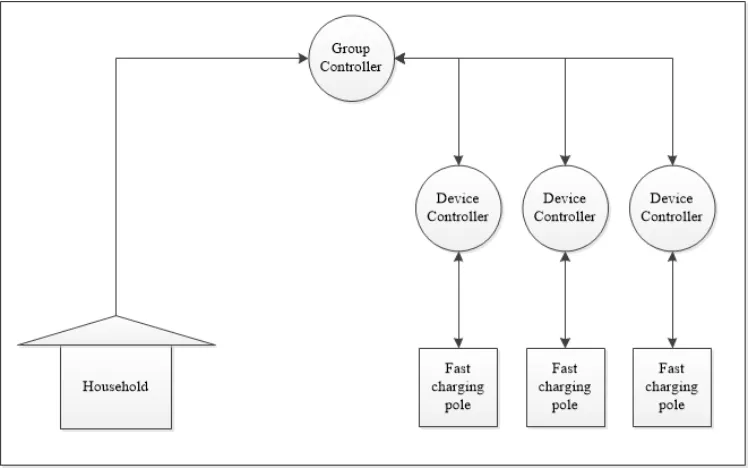
1. Group controller, all devices and load-flow simulator request control round(s) from the simulation controller. Group controller gets round #1; all basic devices (include EVs) get round #2; and load-flow controller gets the next round(s) to get ready and perform its duty.

2. In round #1, the group controller and device controllers work in an iterative way as described later to generate a profile for each controllable device. This control round does not necessarily present in every time interval though. How long a replan will take place depends on the planning horizon and replanning-related parameters of the group controller.

3. In round #2, devices carry out the plan.

4. In the next round, the load-flow controller calculates voltage, current information over the local grid to be used for further analysis.

5. In the last control round, a function of devices are called to store all kinds of information for display. This work flow is also shown in Figure 2.5.

2.2.3 Power peak shaving

To understand the purposes and mechanisms of power peak shaving, what a power peak is must be introduced firstly. Power peak is a relative notion that needs a reference value [15]. This value often refers to a power limit that should not be exceeded. This limit could be based on constraints of the grid,

preferences of end users and power distributors, etc.

Figure 2.5: Work flow of the Triana simulator

Figure 2.6: Power peak shaving performed in a heat pump case, taken from [21]

profile called desired profile. Often set to be flat, this desired profile is reached by minimizing the following formula, Q= v u u t End X t=0

(Pplan(t)−Pdes(t))2 (2.1)

wherePdes(t) represents the desired global active power profile at timet.

This is realized in a hierarchical planning algorithm described in [5]. In this case, controllers, devices, pools and other elements are also modeled and organized hierarchically in the same way as described in section 2.2.1. The master controller is the root controller, which always has multiple child controllers. These child controllers can be either group controllers, which can have their own children or device controllers, which is the leave node.

Once the request of a new plan is given by the master controller, algirithm 2.1 is performed.

Algorithm 2.1Hierarchical profile steering algorithm [5]

1: Master controller request each childm∈ {1, 2, 3..., M} to minimize its power profilek−→xmk₂

2: −→x ←PM

m=1

− →_x

m .Total power profile

3: do

4: −→p ← {Pdes(0), Pdes(1), ..., Pdes(End)}

5: −→d ← −→x − −→p .Difference vector

6: for allm∈ {1, 2, 3..., M} do

7: −→pm← −→xm−

− →

d

8: For each childmfind a new planning−→xˆm that minimizes

− → ˆ

xm− −→pm

₂

9: em← k−→xm− −→pmk₂−

− → ˆ

xm− −→pm

₂ .Relevant flexibility ofm

10: end for

11: Findmwith the highest contribution em

12: −→x ← −→x − −→xm+

− →

ˆ

xm .Update total profile

13: −→xm←

− →

ˆ

xm . Update the profile of m

14: while em< .Repeat as long as there is sufficient progress

Basically algorithm 2.1 tries to reduce the difference betweenPplan andPdesin an iterative way. In each

Then it loops over all of its children in order to find a winner that can provide the most flexibility given its current plan. Once it is found, the winner will adopt its new plan. As a resultPplan is improved at the end

of each iteration. This iterative process repeats until the convergence criteria are met. In this case, if the number of iterations is larger than permitted or the flexibility given by the winner in one iteration is lower than the preset value (), the iteration process terminates.

During the planning stage, an optimal global power profile is found which remains as close toPdes as

possible according to the proximity factorQin Equation 2.1. In this way, power peak shaving at LV network level is accomplished.

2.3

Network modeling

2.3.1 Lochem

As discussed in Chapter 1, to validate the designed architecture, it is applied into the simulation using Triana network model of Lochem. Previously two stress tests have been conducted there to study the effect of peak demand caused by high penetration of EVs and plug-in hybrid Electric Vehicles on the local LV grid. After each stress test a Triana network model corresponding to the test site settings was made and then validated with load-flow simulation [8]. Therefore in simulation the validity of Triana network model is guaranteed.

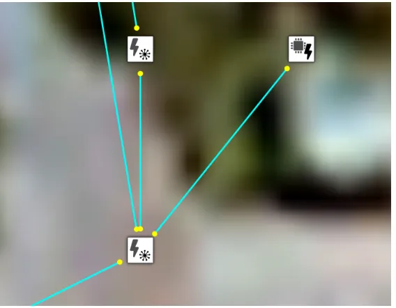
Figure 2.7 gives an overall view of the model. It can be seen that all households are connected to a master controller in the center by red wires, which represent control connections. Zooming in, it is clear that a cluster of red wires is actually the control connections between master controller and device

controllers of individual household as shown in Figure 2.8. There is a LV network node in every household, represented by a lightening symbol. It has all kinds of voltage properties and is the gateway to local LV grid. Blue wires in the picture represent low voltage cables connecting households to local LV network. These blue wires as well as LV network nodes form a local LV grid, “powered” by a transformer which is also modeled as a LV network node. It is connected to a simulation controller symbolized with a chip in Figure 2.9. The simulation controller is used to simulate the network and manage all statistics.

Figure 2.7: An overall view of the Triana model in Lochem project

Figure 2.8: Modeling of a single household in Lochem project

Figure 2.9: Modeling of transformer and simulation controller in Lochem project

2.3.2 Load-flow simulation

The load-flow simulation module is added as a separate module in the Triana simulator. A definition of load-flow simulation is given in [9].

Definition 2.2 Load-flow calculations on network models are used to obtain voltage levels, distribution losses and other network information for a certain scenario. These calculations are used in network design to validate that the required capacity will be realized.

To use the results of load-flow calculations as the feedback of the Triana simulator, a separate module called load-flow simulator is implemented and added to the Triana simulator. The goal of the load-flow simulator is to determine all voltage levels, angles and power flows in the network. These information can form a steady state of the LV network containing the voltage level at LV nodes, the active and reactive power flowing in the network and the phase angle between voltage and current.

There exists multiple load-flow calculation algorithms. Newton-Raphson [20], Gauss-Seidel and Holomorphic Embedding Load-Flow method [22], to name a few. Among them, the Forward-Backward Sweep [26] is chosen and implemented [9]. It uses Kirchhoff’s Current Law (KCL) and Kirchhoff’s Voltage Law (KVL) and can be used for radial networks. In the Triana model, it works from the slack bus to the end nodes in the forward sweep, calculating the voltage at each node. The voltage levels are calculated based on the voltage drop along the branches. The voltage drop is caused by the impedance of the cables and the current running through them. Then in the backward sweep it works in the opposite direction to calculate the currents running in each cable. This process runs continuously until the convergence criterion is met. This is usually when the voltage levels calculated in two consecutive iterations are close enough.

3

Design Decisions and Real-time Control Algorithm

In the first part of this chapter, design decisions about the real-time control algorithm and the API of Triana to access RTD are made. Later based on those determined strategies, the designed algorithm is presented in section 3.2.

3.1

Design decisions

As listed in Chapter 1, it is essential to answer all sub-questions to find a best design for the real-time control algorithm and API. The Triana simulator has been proven to function as expected in many cases thus it is reasonable to use as much of its code base as possible.

As discussed in Chapter 1, three objectives of this real-time control algorithm are listed below.

ˆ Upon detection, it must be ensured that overloading problem will be solved as soon as possible.

ˆ The overall power profile remains as close to its original plan as possible.

ˆ Charging deadlines of EVs set by end users are not violated.

In addition to these objectives, two other criteria are considered while exploring suitable real-time control algorithms.

ˆ The modeling of the LV network and the planning step of Triana stay intact and act as the reference of the real-time control algorithm.

ˆ If time allows, the algorithm should be extensible to be device agnostic.

With these in mind, when all sub-questions are answered, major design decisions are made at the same time.

3.1.1 Strategy explorations

In Triana, simulation time is divided into discrete time intervals, normally of length 1minuteor

15minutes. Taking 15−minutetime base as an example, if an initial plan is made at the first time index (i.e. interval[0]) and the planning horizon of this plan is 96 indexes ahead (96∗15minutes= 1day), for the following 95 indexes, Equation 3.1 can be checked to see if a replan should be performed.

Letαbe the maximum degree of deviation allowed. When the following standard fails, the real-time control algorithm must react.

Pdev(t)≤Pplan(t)∗α (3.1)

Note that to avoid oscillation, Equation 3.1 can be extended to Equation 3.2 so that the real-time control algorithm is only triggered oncePdev is too large forM consecutive intervals, i.e.,

Pdev(t)> Pplan(t)∗α when T −M < t≤T (3.2)

whereT is the current time interval during simulation.

Time-based control v.s. Event-based control

Although theoretically it is possible to design an event-based real-time controller instead of a time-based one, RTD streams are normally not continuous. In our case, RTD values are only available at certain time interval. Since events are based on those RTD, in this case they can only be triggered at a time base. Therefore their advantage of fast reaction no longer stands. Moreover, Triana itself is time-based as discussed earlier. In other words, to allow an event-based control algorithm, its original code base must be altered dramatically.

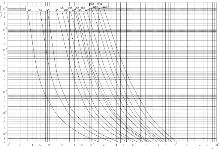
In addition, the most severe case that can happen and cause fatal damages to LV grid is overloading problem. However, The type of fuses used in the feeder of the test site is Jean Muller NH fuse-link. Its rated voltage is 400V AC. With maximum current of 160 A, its time-current characteristics are shown in Figure 3.1. When the feeder is overloaded it can stand current 25% more than its maximum current (200 A in this case) for hours. Therefore even in the most urgent situation it is not necessary to use a event-based

Figure 3.1: Time current characteristics of the fuses used in our use case (source: Jean Muller)

control algorithm.

Based on the reasons aforementioned, the control algorithm is set to be time-based. Since in simulation environment all RTD is available directly for Triana (Figure 1.5), every new control interval they are read and made use of instantly.

Desired profile v.s. Original plan

Although theoretically it is possible to set a desired profile based on previous experience and history usage, in practice, normally in Triana it is good enough to use an empty profile as the desired profile of Algorithm 2.1. (In other words,Pdes(0) =Pdes(1) =...Pdes(End) = 0) If this case applies, the desired

profile gives no further information at all.

Another reason is that Algorithm 2.1 can give an optimal solution minimizing Equation 2.1. Therefore approximating the original planning outcome is approximating the desired profile in some way. Not to mention that the desired profile is not necessarily accessible. For example, substitutingPplanwith Pdes,

Equation 3.1 evolves into:

|Ptotal(t)−Pdes(t)| ≤Pdes(t)∗α (3.3)

If the desired profile is too small at some point (e.g. the aforementioned empty profile), the real-time control algorithm will react much more often than necessary, even introducing oscillations.

Based on those reasons, it is chosen such that the actual overall profile should approximate the original plan (i.e. outcome of the planning step).

Replan v.s. Difference distribution

Before explaining these options in depth, four base scenarios mentioned in Chapter 1 must be analyzed at first. SupposeTpre start(i) andTpre end(i) represent the predicted start and end time of EV charging jobi

respectively andTstart(i) andTend(i) symbolize the real start and end time of jobiindividually, each

scenario can then be detected if its corresponding condition holds, namely,

1. Pdev(t) =Pplan(t)−Pcontrol(t)−Pno control(t), when the uncontrollable loads is lower than its

prediction.

2. Pdev(t) =Pno control(t)−(Pplan(t)−Pcontrol(t)), when the uncontrollable loads is greater than its

prediction.

3. Tpre end(i)> Tend(i), when EVileaves earlier than expected.

4. Tpre start(i)< Tstart(i), when EViarrives later than expected.

To compensate for the deviation in these cases, two types of strategies exist to be chosen from. The first one is replanning, meaning adjusting the original plan (choice of last subsection) according to the deviation and replanning with this adjusted profile as the desired profile. Another option would be to distribute whole or part of the deviation to one or even all of the available EV charging jobs (As described in Chapter 1, only EV charging pole(s) can be controlled in Lochem).

Although the second option seems to be able to compensate the deviation quickly, in the second case where the uncontrollable loads is greater than its prediction, this method will probably cause EV charging deadline violations since to make up for this deviation, EV charging power must be decreased. Therefore later to ensure each EV reaches its deadline, replanning is still necessary.

3.1.2 How to replan the controllable loads to keepPplan0(t) as close toP_plan(t)as possible WhenPtotal(t) satisfies Equation 3.2, there are four possible cases causing the deviation from original

power profile. As discussed in Chapter 1, other scenarios can either be treated as the combination of those four scenarios or be solved by adopting the strategies of these cases. Hence in the remaining of this section those cases are discussed separately to find the most suitable way of replanning.

When uncontrollable load differs from prediction, it is necessary to adjustPplanwithPdev to generate

Pdes0, the desired profile when replanning. The reason is that the deviation of uncontrollable load must be compensated in the new planPplan0; in other words the adjustment ofP_des0 is the adjustment of the predicted uncontrollable profile (Pno control pre). For this reason, it can also be concluded when EV leaves

earlier or arrives later than expected,Pplan can be used asPdes0 without adjustment since the uncontrollable load is the same as expected.

Moreover, when EV leaves earlier or arrives later than predicted, there is no need to check Equation 3.2 since via checking ifTpre end(i)> Tend(i) orTpre start(i)< Tstart(i), whether there will be an undesired

deviation and it cause are already known.

Uncontrollable loads is lower than its prediction

In this case, the planning algorithm 2.1 can be reused. However,Pdes0 must be adjusted according to P_dev. SupposeT is the time when Equation 3.2 stands, at this stage, sincePno control pre(T), the predicted overall

uncontrollable profile at timeT is higher thanPno control(T), from time T, the desired profile Pdes0 can be,

Pdes0(t₁) =P_plan(t₁) +P_dev(T) (3.4)

wheret1∈ {T, T + 1, T + 2..., End}.

Equation 3.4 suggests the prediction thatPdev(T) will last until the end of the simulation. However, this

expectation generally does not stand. Thus parameterK is introduced which symbolizes the predicted length of drop ofPno control from Pno control pre. Hence the extended Pdes0 is,

Pdes0(t₁) =

(

Pplan(t1) +Pdev(T) ift1< T+K

Pplan(t1) ift1≥T+K

(3.5)

Equation 3.5 suggests the real-time control algorithm tries to compensatePdev(T) only for the followingK

time intervals. This strategy is illustrated in Figure 3.2 whereM = 4 and K= 5.

In this example, frominterval[30] tointerval[33] the uncontrollable load is lower than expected for

M = 4 intervals. Therefore atinterval[33], Equation 3.2 stands and replan is necessary. SinceK= 5, from

interval[33] tointerval[37],Pplanis adjusted byPdev(33) to generatePdes0.

However normally the actual length of the drop ofPno control is different from K. WhenK is greater

than the actual length of the drop, no actions can be taken. While whenK is too small,Pdev is only

0 10 20 30 37 40 50 60 70 80 90 6 8 10 12 14

Pdev(33)

Pdev(33)

Time Intervals P o w er [kW] Pplan Ptotal

P_des0

Figure 3.2: Illustration of the strategies adopted in Case 1 atinterval[33]

0 10 20 30 33 38 40 50 60 70 80 90

6 8 10 12 14

Pdev(38)

Pdev(38)

Time Intervals P o w er [kW] Pplan Ptotal

P_des00

Figure 3.3: Illustration of the strategies adopted in Case 1 atinterval[38]

To allow this fast reaction,F is introduced. It is a flag representing whether it is a lasting uncontrollable power drop/ peak. Once Equation 3.2 stands,F is set toDROP (unpredicted uncontrollable power drop) orP EAK (unpredicted uncontrollable power peak). OncePno control pre=Pno control,F is set to its

default value,N ON E. The introduction ofF means that even ifKis much smaller than the actual length of the uncontrollable load deviation, it is still possible to compensate for it till its end via performing multiple replannings.

Uncontrollable loads is greater than its prediction

In this case, the strategy adopted is the same as that adopted in the last case. One exception is that Equation 3.5 should be replaced with Equation 3.6 becausePdev is the absolute difference betweenPtotal

andPplan.

Pdes0(t1) =

(

Pplan(t1)−Pdev(T) ift1< T+K

Pplan(t1) ift1≥T+K

As a result, the example in the last case evolves into what is shown in Figure 3.4 and Figure 3.5.

0 10 20 30 37 40 50 60 70 80 90

6 8 10 12 14

Pdev(33)

Pdev(33)

Time Intervals P o w er [kW] Pplan Ptotal

P_des0

Figure 3.4: Illustration of the strategies adopted in Case 2 atinterval[33]

0 10 20 30 33 38 40 50 60 70 80 90

6 8 10 12 14

Pdev(38)

Pdev(38)

Time Intervals P o w er [kW] Pplan Ptotal

P_des00

Figure 3.5: Illustration of the strategies adopted in Case 2 atinterval[38]

However, different from the last case, when replanning is performed, the charging power of EVs is highly likely to decrease. Therefore, it might introduce charging deadline violations. To balance between

obtaining a desired profile and charging EVs on time, Equation 2.1 in Algorithm 2.1 is extended to tolerate EV charging deadline violations,

ˆ Q= v u u t End X

t=T

(Pplan0(t)−P_des0(t))2+γ∗

N

X

i=1

(Dext(i)−D(i)) (3.7)

where there areN EVs in total,D(i) andDext(i) represent the charging deadline and the actual finish

By extending Equation 2.1 with penalty for EV charging delay, during simulation it can be set whether it is preferred to suffer from EV charging deadline violations in exchange of a more flat overall profile. As a result, Algorithm 2.1 can not only be performed when every EV meets its deadline, but also be used when the delayD∈ {1, 2, 3..., ∞}is applied for each EV.

The strategies taken in this case can be concluded as Algorithm 3.1,

Algorithm 3.1The strategies applied when uncontrollable load is greater than expected

1: calculate Pdes0 according to Equation 3.6

2: Save all available EV charging jobs into a list L

3: Use Algorithm 2.1 withPdes0

4: Delay D←0

5: while D≤M AXIM U M DELAY ALLOW EDdo

6: D←D+ 1

7: if L is not emptythen

8: Extend the charging deadline of each EV charging job inLbyD

9: Use Algorithm 2.1 withPdes0, replacing step 9 of Algorithm 2.1 with Equation 3.8

10: Remove charging jobs making no contribution to Equation 2.1 fromL

11: else

12: break

13: end if

14: end while

In Algorithm 3.1, the introduction of the maximum delay allowed for all EVs

(M AXIM U M DELAY ALLOW ED) and the list of all EV charging jobs (L) form two convergence criteria, namely,

ˆ DelayD keeps increasing untilD≥M AXIM U M DELAY ALLOW ED, Algorithm 3.1 ends.

ˆ Every timeD increases, the planning algorithm is performed again. After this planning process, if a EV charging job does not obtain a new plan (making no contribution to Equation 2.1), it is removed from L. WhenLis empty, Algorithm 3.1 stops.

In addition, for step 9 of Algorithm 3.1, when calculating the flexibility of each EV, penalty for deadline extension is included according to Equation 3.7. Therefore when using the planning algorithm, step 9 must be replaced with Equation 3.8.

em← k−→xm− −→pmk2−

− → ˆ

xm− −→pm

₂−γ∗(Dm−

ˆ

Dm) (3.8)

whereDmis the delay of plan−→xmand ˆDmis the delay of plan

− →

ˆ

xm.

Algorithm 3.1 can also be found as part of the real-time control algorithm in section 3.2.

EV(s) leave earlier than expected

In this case, the planning algorithm 2.1 can be reused for other EV charging jobs. Suppose EVj leaves earlier than expected, by design replan should only happen once when EVj actually leaves. In other words, atTend(j), a replan should be performed without EVj. Thus in the new plan, the charging power

EV(s) arrive later than expected

Suppose EVj arrives later than expected, when time reaches the predicted arrival time of EVj, the action performed when EV leaves earlier than expected can be reused. This means by design a replan without EV

j should happen firstly atTpre start(j). Then atTstart(j), EVj can then be made available and the second

replan with all current EV charging jobs at the moment is necessary. Hence in theory, two replans are made in this case. The original overall plan can also be used as desired profile in both replannings without being adjusted.

3.1.3 Necessary measurement data

As described in Chapter 1, the major use case of this master thesis assignment is to detect and solve prediction/ planning errors. To inform the Triana simulator of this problem in time, RTD of transformers and feeders must be sent to it. This section will discuss which RTD is essential to fulfill this task. Since LV grid is the focus of the Triana simulator when monitoring prediction/ planning errors, only the outgoing field of transformers and the feeders connected to it will be metered in our case. The measurement points for one transformer are shown in Figure 3.6.

Figure 3.6: Measurement points for one transformer in this project

As shown in the picture, voltage of the secondary side of the transformer and current of all feeders connected to it can be measured. To be specific, the necessary RTD per phase for each measurement point is,

ˆ power (active power)

In addition, line - neutral voltage of each phase must be provided as well if wanting to perform load-flow simulation.

ˆ power (reactive - and apparent power)

ˆ phase angle

ˆ current

In the Nahanni shared memory, each RTD is labeled with a unique ”path” (e.g. /bay/01/current/L1). Based on those RTD, it is then possible to detect the problem in the LV grid as expected.

3.1.4 Scheduling memory access

Nahanni supports spinlocks which can monitor a value in shared memory [12]. Therefore, polling mechanism with primitives built upon spinlocks are clearly an option for synchronizing memory access between VMs. An alternative is to use interrupt to notify other VMs. As discussed in [12], the

introduction of Shared-Memory Server makes it possible. Another inter-VM communication method often discussed is direct memory access (DMA). However, it is not possible to implement it in Nahanni given only a DMA engine. All possible options need to be compared to select the most suitable one.

Polling

Polling is the process where the computer or controlling device waits for an external device to check for its readiness or state, often with low-level hardware [25]. In our case, if an application tries to access a resource in the shared memory which is currently being used by another application in another VM, it will ”spins” around the spinlock waiting until it is released so that the resource is free to access.

Interrupt

Interrupt, in [19], is defined as a hardware mechanism that enables a device to notify the CPU. In our case, this mechanism is useful when an application intends to notify other applications running in other guest OSes about the availability of resources in the shared memory. More details about the process of interrupt sending and receiving in Nahanni can be found in [12].

Comparison

As described in section 3.1.1, the transmission of RTD does not necessarily have to be frequent. Moreover, when to access the shared memory is known beforehand. Hence polling is considered a sufficient option in our case.

3.2

Real-time control algorithm

As discussed before in this chapter, there are four base cases acting as the target of the real-time control algorithm, namely,

1. Case 1, when the uncontrollable loads is lower than its prediction. 2. Case 2, when the uncontrollable loads is greater than its prediction. 3. Case 3, when EV(s) leave earlier than expected.

4. Case 4, when EV(s) arrive later than expected.

Based on the these cases and design decisions aforementioned, a real-time control algorithm is

Algorithm 3.2A real-time control algorithm in Triana

1: At the start of a new time interval T(i.e. 15minute)

2: Get RTD values via RTD module from the shared memory

3: if Pdev(t)> Pplan(t)∗αwhenT−M < t≤T orF ==DROP &&Pplan(T)−Ptotal(T)> Pplan(T)∗α

or F ==P EAK && Ptotal(T)−Pplan(T)> Pplan(T)∗αthen

4: if Pplan(T)> Ptotal(T)then

5: F ←DROP

6: Pdes0(t) =P_plan(t) +P_dev(T)∗β whenT+K > t≥T;P_des0(t) =P_plan(t) whent≥T +K

7: Perform the same planning algorithm with Pdes0

8: else

9: F ←P EAK

10: Pdes0(t) =P_plan(t)−P_dev(T)∗β whenT+K > t≥T;P_des0(t) =P_plan(t) whent≥T +K

11: Save all available EV charging jobs into a listL

12: Use Algorithm 2.1 withPdes0

13: DelayD←0

14: while D≤M AXIM U M DELAY ALLOW EDdo

15: D←D+ 1

16: if Lis not empty then

17: Extend the charging deadline of each EV charging job inLbyD

18: Use Algorithm 2.1 withPdes0, replacing step 9 of Algorithm 2.1 with Equation 3.8

19: Remove charging jobs making no contribution to Equation 2.1 fromL

20: else

21: break

22: end if

23: end while

24: end if

25: else

26: F ←N ON E

27: end if

28: if In Case 3, EV leaves or in Case 4 EV is expected to arrivethen

29: Perform Algorithm 2.1 with all available EV(s) for the remaining planning horizon

30: end if

31: if In Case 4, EV actually arrivesthen

32: Perform Algorithm 2.1 with all available EV(s) for the remaining planning horizon

33: end if

4

Simulation Results and Analysis

In this chapter, the common simulation environment of all cases will be introduced at first. Followed are detailed settings of each case and the simulation results of each case. Based on the effect of the algorithm, analysis is made on each case separately. Finally, a general conclusion is drawn based on all matters above.

4.1

Use case

As discussed in Chapter 2, the Triana network model of Lochem is provided. As the stress test conducted on 2nd of April, one of the four feeders in Lochem is tested. The transformer installed on Mauritsweg provides electricity for 71 households and three fast charging poles connected to this feeder. As mentioned in Chapter 1, the predicted uncontrollable profile is generated by the profile generator developed by G.Hoogsteen. In Figure 4.3 (red dotted line), it can be seen that the profile generated by it resembles what one normally expects from the total power consumption of dozens of households during weekend.

To read the power consumption of each household, an uncontrollable device controller/ reader is connected to each household, as shown in Figure 4.1. To plan and control EV charging jobs in each fast charging pole, a buffer time shiftable controller is connected to each of them. A master controller, the parent of all those controllers, is responsible for global planning and control. All control connections are shown in Figure 4.1.

Figure 4.1: Illustration of Triana modeling and control connections of the use case

The whole simulation process is divided into 96 consecutive time intervals. Since the duration of the simulation is one day, the time base of each interval can be calculated by,

T ime base= 24hours/96 = 15minutes (4.1) In the simulation, at time interval 0, an initial plan is made for all devices. At every following interval, if Equation 3.2 stands, the real-time control algorithm discussed in section 3.2 will start to work. In the following section, the effect of this algorithm will be discussed in all four aforementioned cases as well as in a more realistic case where uncontrollable load shifts over time.

To allow quantitative measurement of the proximity ofPtotal with regards to the original plan,

Equation 2.1 can be rewritten as,

Q0 =

v u u t End X t=0

(Ptotal(t)−Pplan(t))2 (4.2)

whereEndrepresents the last time interval of simulation (e.g. 95 in the simulation).

In cases when EV charging deadline extension is involved, similar to Equation 3.7, Equation 4.2 can be extended into,

ˆ

Q0₌

v u u t End X t=0

(Ptotal(t)−Pplan(t))2+γ∗ N

X

i=1

(Dext(i)−D(i)) (4.3)

where there areN EV charging jobs in total. With Equation 4.2 and Equation 4.3, it is then possible to evaluate the performance of the real-time control algorithm by comparing ˆQ0 _{between with and without}

Algorithm 3.2 with Equation 4.4,

Improvement= ( ˆQ0

no rtc−Qˆ0rtc)/Qˆ0no rtc∗100% (4.4)

where ˆQ0

no rtc represents ˆQ0 when Algorithm 3.2 is not introduced and ˆQ0rtcis ˆQ0 when the real-time

control algorithm is performed. With Equation 4.4 it is possible to calculate the improvement of ˆQ0

brought by Algorithm 3.2.

Although theoretically it is possible to achieve 100% improvement of ˆQ0 _{in Equation 4.4, in cases where}

the energy consumed byPplandiffers from that consumed byPtotal, the maximum improvement is lower.

SupposePoptimal is the overall power profile that realizes maximal improvement, it can then be gained by

evenly spreadingPEnd

0 Pplan−

PEnd

0 Ptotal from the first interval whenPtotal differs fromPplan to the end

of the simulation (e.g. interval[95] in our case), as illustrated in Figure 4.2.

In the example shown in Figure 4.2, frominterval[30], Ptotal starts to deviate from Pplan till

interval[50]. The optimal solution as described before would spread the total amount of deviation to the remaining simulation time (i.e. interval[30] tointerval[95]), shown asPoptimal in Figure 4.2. As

demonstrated in Figure 4.2, the integral ofPtotal is the same asPoptimal, which proves that under the

assumption that EV charging deadlines and the shape of uncontrollable loads are not taken into account,

0 10 20 30 40 50 60 70 80 90 0

5 10 15

Time Intervals

P

o

w

er

[kW]

Pplan

Ptotal

Poptimal

Figure 4.2: Illustration of the optimal overall power profile achieving maximal improvement

4.2

Results and analysis

4.2.1 Case 1: uncontrollable load is lower than predicted

(Predicted) Start time (Predicted) End time Max charging power[kW] Capacity and Setpoint[kWh]

EV 1 45 60 17.1 30

EV 2 50 80 14.1 66

EV 3 50 70 17.1 51

Table 4.1: Detailed information of all EV charging jobs

The detailed settings of EV charging jobs in this case can be found in Table 4.1. In order to create an unexpected uncontrollable power drop, from timeinterval[50] tointerval[70], the real uncontrollable load is 0.65 times the predicted uncontrollable load in all three phases. This is shown in Figure 4.3.

0 10 20 30 40 50 60 70 80 90

6 8 10 12 14 16

Time Intervals

P

o

w

er

[kW]

predicted uncontrollable load L1 real uncontrollable load L1

In the experiment, beforeinterval[54], the real-time control algorithm never performs replanning. At

interval[54], due to the changes in Figure 4.3, Equation 3.2 stands (M = 4). Therefore the 1st replanning is performed. This new plan, according to Algorithm 3.2, tries to compensate for the next 5 intervals (K= 5) the deviation caused by wrong prediction of uncontrollable loads. As a result, after 5 intervals, Equation 3.1 is violated again atinterval[59]. It is then decided that the length of the deviation of uncontrollable loads is longer than expected (K). Thus the 2ndreplanning with the same strategy as the 1st _{one is performed. For the same reason, the 3}rd _{replanning is done atinterval[64], i.e. 5 intervals after}

the last replan. These replan times can also be found in Figure 4.4.

0 10 20 30 40 50 60 70 80 90

0 2 4 6 8 10

Time Intervals

Times

replan times (accumulated)

Figure 4.4: How many times replan has taken place (accumulated)

Then atinterval[65], EV 3 is almost fully charged (46121.3/51000 = 90.4%), as can be seen in Figure 4.5. Thus the potential of it to compensate the ”missing” part of uncontrollable load is limited. This is when the first oscillation happens. Frominterval[65] tointerval[70], Algorithm 3.2 fails to compensate this decrease of uncontrollable load at every time. Therefore replan times keep increasing as shown in Figure 4.4.

0 10 20 30 40 50 60 70 80 90

0 10 20 30 40 50

Time Intervals

P

o

w

er

[kW]/

En

e

rgy

[kWh]

Active power demand State of Charge

Then atinterval[78] and interval[79], since EV 2 has also finished its charging (its deadline is 80 but it finishes earlier atinterval[75] as shown in Figure 4.6), the new plan is much lower than the original plan (Figure 4.7). However, even though at both intervals Equation 3.1 is violated, nothing can be done because no controllable loads are at disposal.

0 10 20 30 40 50 60 70 80 90

0 20 40 60 Time Intervals P o w er [kW]/ En e rgy [kWh]

Active power demand State of Charge

Figure 4.6: Active power demand and state of charge of EV 2

0 10 20 30 40 50 60 70 80 90

6 8 10 12 14 16 Time Intervals P o w er [kW]

original power plan L1

original power plan in real case L1 executed power plan L1

Figure 4.7: Original plan (predicted and real life) and final executed plan of phase 1

In Figure 4.7, it is shown that compared with taking no actions (blue dashed line), the new plan (black solid line) stays more close to the original plan (red dotted line). This can be proved using Equation 4.4. It can be calculated that the new planning can improve the proximity factorQ0 by 2.7%