A Process Model for
Remote Sensing Data Analysis
Varun Madhok and David A. Landgrebe,
Life Fellow, IEEE
Copyright © 2002 IEEE. Reprinted from IEEE Transactions on Geoscience and Remote Sensing. Vol. 40, No. 3, pp 680-686, March 2002.
This material is posted here with permission of the IEEE. Such permission of the IEEE does not in any way imply IEEE endorsement of any of Purdue University’s products or services. Internal or personal use of this material is permitted. However, permission to reprint/republish this material for advertising or promotional purposes or for creating new collective works for resale or redistribution must be obtained from the IEEE by sending a blank email message to [email protected].
By choosing to view this document, you agree to all provisions of the copyright laws protecting it.
A Process Model for
Remote Sensing Data Analysis
Varun Madhok and David A. Landgrebe,
Life Fellow, IEEE
Abstract -- Remote sensing data is collected and analyzed to enhance understanding of the terrestrial surface– in composition, in form or in function. One approach to accomplishing this is by designing the analysis process as an iterated composite of several analyst-directed modules. This paper proposes such a modular design for the data analysis. The proposed methodology was applied in a project to obtain the thematic map for a flightline over Washington D.C. with very satisfactory results– the qualification being in both the visual and the statistical sense. The project execution is presented as a case study in this paper.
Index Terms -- methodology, masking, segmentation, digital elevation map, human-computer interaction, holistic solution, hyperspectral data classification.
I. INTRODUCTION
HE foundation of this paper is the proposition that effective multispectral image data analysis is an analyst driven placement of algorithms in which mathematical rigor, though of fundamental importance, is secondary to the analysis process. Practical engineering applications demand solutions that are robust across diverse projects. However, the performance of an analysis algorithm is dictated by its fit to the problem context. An algorithm tuned in to a particular context is unlikely to be as effective in another scenario. Such practical issues nearly always preclude the existence of turn-key solutions for practical problems requiring remote sensing data analysis. On the other hand, principles of solution design are equally applicable across diverse projects. Identification and organization of these principles into an analysis methodology is the motivation for this paper.
Section II of this paper discusses related research and proposes a methodology for remote sensing data analysis. Section III demonstrates how this methodology has been successfully applied in a classification analysis of data collected for a flightline over Washington D.C.
Manuscript received February 23, 2001. The work described in this paper was sponsored in part by the U.S. Army Research Office under Grant Number DAAH04-96-1-0444.
Varun Madhok is with the Analytic Value Creation Practice, IBM Canada Ltd., Markham, ON L3R9Z7, Canada (e-mail: [email protected]).
David A. Landgrebe is with the School of Electrical and Computer Engineering, Purdue University, West Lafayette, IN47907-1285, USA (e-mail: [email protected]).
II. REMOTE SENSING DATA ANALYSIS A. Related Work
The philosophy of this paper’s discussion is embodied in a work by Kushnier, et al. [1] in the context of military strategizing. The authors state that the task of making tactical decisions in naval operations is too complex to be accomplished by humans alone or by computers alone, and present several examples in support of the statement. The paper highlights the division of responsibilities between person and machine with the proposition that the human uses judgment and native intuition to make decisions while the assessment of the situational physics is a highly mathematical endeavor best left to the computer. Also of note is the work of McKeown, et al. [2] for cartographic feature extraction. Their design echoes the methodology and the principles discussed in this paper.
B. Design principles
Mathematical modeling on the computer serves a useful purpose, in that the system dynamics can be reduced to the manipulation of a few parameters. If applicable, the complexity of the ensuing analysis can be significantly reduced, and thus be synthesized by the user into a suite of analysis-routines. In contrast, the factor invaluable to the successful application of laboratory models of terrestrial phenomena is the human ability to learn and to adapt the analysis to the peculiarities of the problem. Successful analysis is thus a balance between perceptive insights and mathematics. The principles at core of the proposed methodology are listed as axioms below.
Axiom 1: Human abilities are different from those of the computer.
Consider Table I, adapted from [3]. The conclusions drawn from Table I are that the inferential aspects of the analysis are best left to the human. On the opposite side, the computer's superiority lies in executing number crunching applications of analyst design.
Multispectral1 remote sensing image data convey
information at the elemental level through energy spectral/spatial measurements, and at the composite level through inter-pixel relationships. The subjective evaluations afforded by the image representation are the interface between the human and the computer - thus the
1 By multispectral image data is meant data gathered over a scene on a pixel by pixel basis to constitute an image in which measurements are made for each pixel in a few to perhaps several hundred individual regions of the electromagnetic spectrum.
computational analysis is guided by analyst assessment of the visualization. This perspective is key to initiating and guiding remote sensing data analysis. The ensuing discussion does not suggest a design of intelligent/learning algorithms or of automated solutions. The emphasis lies on the recognition of human-computer interaction as a master-drudge relationship and the utilization of the respective strengths in the design of a holistic solution.
Axiom 2: The machine (in)validates the user's hypothesis.
In various applications, the output of the algorithm is a measure of belief in the hypothesis posed by the analyst. A poor output does not necessarily imply algorithmic deficiencies. Failure is often a result of the algorithm and/or the performance metric being unsuitable to the objective. Mathematical analysis is usually directed by the optimization of a user-defined performance measure. Incompatibility between this measure and the objective is unlikely to produce the desired results. In regard to analyses that seek a visual interpretation of the data, this is an especially important issue. Algorithms that process spatially organized data through the optimization of mathematical criteria are often sub-optimal in the sense that the output image is cluttered (or fuzzy or noisy) and is visually unpleasing.
Axiom 3: Every analysis usually requires at least one revision.
Usually, analysis is comprised of various algorithmic 'objects', selected from a suite of procedures, linked in the appropriate sequence by the analyst. The optimal selection and ordering of these objects is often not known. Occasionally, algorithm parameterization is also dependent on human input. Any test run of the process is likely to produce results that can be improved upon through experimentation. Furthermore, analytical models for natural phenomena are approximations to an ideal that is never encountered in practice. Their performance in remote sensing data analysis is sub-optimal.
The corollary to Axiom 3 is that practical engineering problems cannot be solved perfectly. The termination of analysis depends largely on the tolerance level for errors, the available resources, and the available time. Solution implementation requires experimentation with a multitude of analysis algorithms. The best solution is often a patchwork of several techniques pieced together to meet the critical success factors. Additionally, this postulate does not downplay the need for fundamental research for new algorithms and techniques. It proposes that the performance of the ‘best’ automated solution always can benefit from tuning to fit the problem context.
C. The methodology
There are three phases to the implementation of every remote sensing data analysis project. Each of the phases comprises several activities. These phases (bulleted with ‘P’), and the associated activities (bulleted with ‘A’) are listed below, in order of occurrence.
P Problem Definition.
A Objective identification.
A Success metrics definition / statement of completion criteria.
A Constraints identification. P Solution Definition.
A Data source(s) identification. A Algorithm-suite compilation. P (Iterative) Solution Implementation.
A Data preparation.
A Algorithm implementation. A Results assessment.
The phases and the associated activities listed above will be explained through the case study in the next section.
III. CASE STUDY – ANALYZING THE D.C. FLIGHTLINE A. Preface
The standard assumption in remote sensing data analysis is that measurements on the energy reflected or emitted from the Earth’s surface contain the information from which the corresponding terrain-type or land-usage can be identified. Under the belief that the scene comprises a definite set of scene-classes, these data can be processed and each element (pixel) assigned a label from this set. A color representation of the output is known as a thematic map or a classification map, the colors used in the representation being mapped one-to-one with the set of scene-classes. The project described in this section generated a thematic map from the remote sensing data and the Digital Elevation Map (DEM) for a flightline over Washington D.C. using the proposed process model to guide its execution.
B. Project design P Problem Definition
A Objective – The project requires the classification of data collected on a flightline over Washington D.C. into a set of scene-classes that spans the thematic content of the scanned region. For the given data, the thematic content is spanned by the class-set {ROOF, ROAD, SHADOW, TREE, GRASS, WATER, PATH}.
A Success metrics – The primary criterion for task completion is ‘picture quality’ of the thematic map based on subjective evaluation for correspondence of the results with analyst understanding of the scene, and for absence of speckle2
misclassifications. This qualitative assessment is supplemented with a quantitative comparison of the output thematic map and regions in the
2 The term ‘speckle’ is used in a sense different from that used by researchers in radar data processing. In this context, speckle noise represents the ‘salt and pepper’ effect of isolated pixels classified distinctly in a large patch of the scene labeled a certain scene-class. The clutter need not be a spectral misclassification, but may be a logical aberration, e.g. speckle noise due to rain puddles on rooftops.
flightline identified by an independent observer as specific scene-types.
P Solution Definition
A Data sources – The data for this case study were collected using an airborne scanner over Washington D.C. The spatial representation of this data is a region 1310 pixels ¥ 265 pixels. The
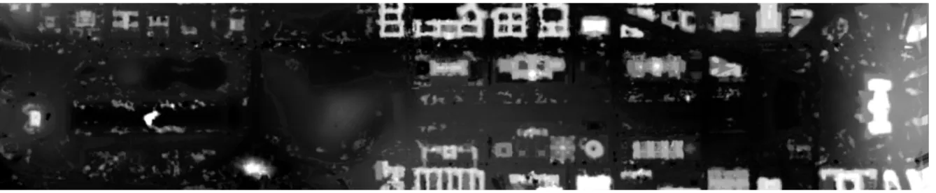
airborne scanner gathered data in each pixel over 210 channels (samples of the energy spectrum) between 0.4 and 2.4 mm. A three color representation of these data is shown in Fig. 1. An additional source of information was the Digital Elevation Map (DEM) of the scene. The grayscale representation of the DEM is shown in Fig. 2. The range for the elevation map was 0.5m to 55m. A Algorithm suite – The analysis suite comprised an
algorithm for quadratic maximum likelihood classification, an algorithm for segmentation of spectral data using a stochastic image model, and several improvisations to process the thematic map and the DEM. Details on these techniques are obtainable at [4].
P Solution Implementation
A Data preparation– The 210 spectral channels3 of data were individually examined for noise. It was observed that physical defects in the scanner, detector saturation and water absorption bands had corrupted several spectral channels. These data were excluded from the analysis. 104 of the original 210 channels were retained for the analysis.
A Algorithm implementation– The solution required several iterations of algorithm implementation and output assessment. The output assessment at the end of each cycle was a visual examination of the thematic map generated at the end of the algorithm execution. The quality issues were addressed in the same sequence. An important design innovation was a “masking” scheme to exclude data that had been correctly classified from subsequent processing. This innovation enabled a consistent improvement in output quality in stepping through the analysis-assessment cycles. A representation of the solution implementation is shown in Fig. 3. Each oval in the graph corresponds to a particular implementation-assessment cycle, and is labeled a ‘Node’. The analysis was initiated at the ‘Root node’. Successive nodes are labeled ‘Node 1’, ‘Node 2’, ‘Node 3’, … These nodes are briefly described in the Appendix. Further details may be obtained at [4].
A Output assessment - The output at each iteration of the analysis is a thematic map that was generated
3The channel number, as in this usage, signifies a specific wavelength at which the spectrum of energy reflected from the Earth has been sampled. Correspondingly, the 210 channels for the scanner are representative of samples at 210 distinct wavelengths.
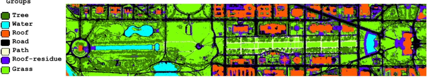
using MultiSpec [5]. The iterations were terminated after Node 8. The final output is shown in Fig. 4. It passed the subjective evaluation criteria- absence of clutter, verification by regional expert for absence of logical aberrations in classifications. This output was validated against test data identified in Fig. 5. These test data were gathered by a researcher4 independent of the
analysis presented here, as representative samples of each scene-class in the flightline. The output in Fig. 4 could thus be compared to the test data identified in Fig. 5 to evaluate the accuracy of the analysis. The final classification at Node 8 is assessed in Table II for each of the scene-classes. For comparison, Table II also lists the classification performance at the Root Node. Note the jump in classification accuracy from 87.3% to 94.3%5. Note also that the accuracy improvement
in the proposed design is a directed approach – the pixels whose classification accuracy is to be improved are processed independent of the remaining data. This explains why the nodes are listed along with the scene class in the listing for the final output.
IV. DISCUSSION
The premise of the proposed methodology is that the current suite of analysis algorithms is sufficient to handle practical remote sensing data analysis problems. Indeed, minor modifications to existing algorithms for specific projects are samples of the innovation driven approach emphasized in this paper, rather than new inventions.
The proposed methodology is also important in two practical respects.
· It promotes collaboration across diverse disciplines by focusing the respective specialists on specific issues in the project. For instance, the School of Civil Engineering at Purdue University, using technology of BAE Systems of San Diego, California, generated the DEM for the project presented as a case study in this paper.
· It enables project management in practical industrial applications of remote sensing data. The project breakdown proposed here can be used to balance timelines, money and human resources against the achievement of the success criteria.
We believe that the incremental value of developing sophisticated data analysis algorithms is negated by the difficulty of disseminating the knowledge required to use
4 Y. Zheng, private communication. Y. Zheng was with Purdue University.
5 The scene-class ROOF, has been characterized in the functional sense in Node 8. If scene-class ROOF-RESIDUE is merged with ROOF, the number of pixels in Node 8 correctly identified as the functional class 'roof' jumps to 1174, and the overall classification accuracy improves to 97.19%.
them effectively. In order for remote sensing science to yield the greatest value to society and to business, it is critical that data analysis becomes accessible to the layperson who may have the data access and the analytical ability but not necessarily the mathematical background to delve into algorithmic minutiae. Such a user should be able to design applications around solution objects whose workings need not be understood so long as they produced value. In any case the incremental value produced by a not-perfect analysis would be a quantum leap over the status quo. This is not to say that currently there are no practical (and effective) implementations of remote sensing science. We are proposing that given the few ‘experts’ in the field, the penetration of this technology would be much greater if the non-expert could use remote sensing data analysis to his/her advantage without ‘expert’ guidance. A robust process model is thus far more important to the solution than tinkering with analysis algorithms. It is hoped that this paper will influence the thinking in the community into the same direction.
APPENDIX Root Node – spectral classification
A three-color representation of the multispectral data using channels 60, 17 and 27 (data gathered at wavelengths 0.75µm, 0.46µm and 0.5µm respectively) is shown in Fig. 1. The analysis for the Root Node stepped through the following path.
· A comprehensive set of sceneclasses was identified -{ROOF, RO A D, SH A D O W, TREE, GRASS, WATER, PATH}.
· Training data representative of each of the scene-classes was selected. The scene-scene-classes ROOF and ROAD were realized as being a cumulative of several spectrally distinct sub-classes. Consequently, the set of scene-classes was enlarged to {ROOF1, ROOF2, ROOF3, ROOF4, RO O F5, RO O F6, RO O F7, RO O F8, ROAD1, ROAD2, SHADOW, TREE, GRASS, WATER, PATH}. Fig. 6 is a representation of the training data.
· The discriminant analysis feature extraction technique [6][7] was used to reduce the dimensionality of the data on a class-conditional basis.
· The method of quadratic maximum likelihood classification was used to classify the spectral data to generate the thematic map. The results of the classification are shown as a thematic map in Fig. 7. Note that the sub-classes of ROOF, and those of ROAD, have been merged into their respective groups.
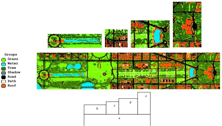
· Sections of Fig. 7 are enlarged as Fig. 3.7b-e, to highlight the errors that need to be rectified in subsequent iterations of the analysis. The errors in classification are surmised to be a result of spectral similarities among various groups of scene classes, namely {ROAD, ROOF, PATH}, {WATER, SHADOW} and {TREE, GRASS}. Output quality could also be
improved by ridding the thematic map of speckle clutter.
Node 1 - WATER + SHADOW separation
Though there was confusion in separating WATER from SHADOW, the discrimination of these from other classes was accurate. To enhance the quality of separation between WATER and SHADOW, the data for these spectral classes were ‘masked’ out from the remainder of the data and run through several iterations of binary segmentation.
Node 2 – SHADOW segmentation
SHADOW was identified as a composite of several sub-classes comprising low energy responses on diverse materials. It was decided to process the data labeled SHADOW in isolation and separate them into spectrally distinct sub-classes. As before these data were masked out and the binary segmentation scheme was applied. Several iterations were performed, and visual quality of the output was the evaluation criterion in each cycle. One of the SH A D O W sub-classes corresponded uniquely to water bodies. This new scene-class was labeled WATER2.
Node 3 - GRASS and TREE separation
From the output at the Root Node, Fig. 7e, it was evident that there was confusion in separating GRASS and TR E E data. The data for these scene-classes were masked out from the remainder of the scene and the unsupervised segmentation algorithm was applied to re-separate the merged classes into TREE and GRASS.
Node 4 – Rooftop extraction
While the definition of a roof implies "the cover of any building" [8], such a functional characterization is complicated to implement via spectral analysis. The ROOF identification in the output of Fig. 7 is mediocre. The digital elevation map (DEM) of the scene captured the functional aspect of the scene-class and was used to enhance the output in this node. A grayscale representation of the DEM is shown in Fig. 2. The lighter pixels in the image correspond to elements at higher elevations in the scene.
The DEM provided information on the rise in elevation of a given area-element in relation to its neighbor. Pixels classified as ROAD, PATH, ROOF or SHADOW were filtered on the corresponding elevation data to isolate rooftops (in the functional sense). Data that had previously been spectrally labeled as ROOF, but were not so labeled after the filtering operation were assigned the class label ROOF -RESIDUE. Details on this analysis are available in [9]. Node 5 – Removal of PATH clutter
To clean the output of speckle clutter, it was decided to forego the use of the spectral data completely. Data quality is a function of the objective, and in this project, debris and traffic (for instance) contributed to noise. While the statistical classification was true to the remote sensing data, the returned output was visually cluttered. In this case, all
PATH classification outside a strip running through the center of the flightline were considered erroneous. These mis-classifications were re-labeled the scene-class that was next closest in spectral similarity.
Node 6 – Removal of WATER2, WATER clutter
It was decided to restrict the spectral classification of scene-classes WATER and WA T E R2 to the large water bodies that could be visually identified in Figure 1. These water bodies are spatially restricted to two rectangular regions on the left and to a small patch in the right part of the flightline. As at Node 5, any data labeled as WATER or WATER2 outside these regions were re-assigned to the next most similar scene-class.
Node 7 - SHADOW re-assignment
It was concluded that the scene-class SH A D O W was temporal, was non-informative, and had to be removed from the output. The maximum likelihood classification algorithm was used to re-assign data labeled SHADOW to other scene-classes.
Node 8 – Removal of WATER clutter
Because of the high spectral similarity (low magnitude of response) between the class SHADOW and WATER, most of the re-assigned data in Node 7 got classified as WATER. The operation similar to that at Node 6 was applied to remove the occurrences of water classification outside the regions identified as water bodies.
REFERENCES
[1] S. D. Kushnier, C. H. Heithecker, J. A. Ballas and D. C. McFarlane, "Situation assessment through collaborative human-computer interaction", Naval Engineers Journal, vol. 108, no. 4, pp. 41-51, July 1996.
[2] D. M. McKeown, Jr. , S. D. Cochran, S. J. Ford, J. C. McGlone, J. A. Shufelt and D. A. Yocum, "Fusion of HYDICE hyperspectral data with panchromatic imagery for cartographic feature extraction", IEEE Transactions on Geoscience & Remote Sensing, vol. 37, no. 3, pp. 1261-1277, May 1999.
[3] B. Schniederman, Designing the User Interface: Strategies for Effective Human-Computer Interaction, 2nd ed., Reading
MA: Addison-Wesley, 1992.
[4] V. Madhok, "Spectral-spatial analysis of remote sensing data: An image model and a procedural design", Ph.D. dissertation, School of Electrical and Computer Engineering, Purdue U n i v e r s i t y , A u g u s t 1 9 9 9 . A v a i l a b l e f r o m http://dynamo.ecn.purdue.edu/~landgreb/publications.html [5] L. Biehl, and David Landgrebe, "MultiSpec - A Tool for
Multispectral-Hyperspectral Image Data Analysis", 13th Pecora Symposium, Sioux Falls, SD, August 20-22, 1996. See also http://dynamo.ecn.purdue.edu/~biehl/MultiSpec/ [6] D. A. Landgrebe, "Information extraction principles and
methods for multispectral and hyperspectral image data", in
Information Processing for Remote Sensing, C. H. Chen, Ed. New Jersey: World Scientific Publishing Co., 2000. Also
a v a i l a b l e f r o m
http://dynamo.ecn.purdue.edu/~landgreb/publications.html [7] C. Lee and D. A. Landgrebe, "Analyzing high-dimensional
multispectral data", IEEE Transactions on Geoscience &
Remote Sensing, vol. 31, no. 3, pp. 792-800, July 1993. Also available from
http://dynamo.ecn.purdue.edu/~landgreb/publications.html [8] Webster's Ninth New Collegiate Dictionary, Springfield MA:
Merriam-Webster, 1993.
[9] V. Madhok and D. Landgrebe, "Supplementing
Hyperspectral Data with Digital Elevation", Proceedings of the International Geoscience & Remote Sensing Symposium (IGARSS), June 28 - July 2, 1999. Also available from
The human The computer
• Can draw upon experience and adapt decisions to unusual phenomena.
• Can reason
inductively, and process hierarchically.
• Can generalize from
observations to build analytical models or decision rules for natural phenomena.
• Can generate output
depending on subjective
interpretation of task.
• Is a source of data,
information.
• Can perform repetitive pre-programmed actions. Can execute
computationally complex algorithms.
• Can process several items
simultaneously.
• Can implement the
generalizations.
• Generates output
conforming to doctrines and performance indices based on a quantitative goal interpretation.
• Has short response time,
high speed of
computation, and cheap data storage.
TABLE I
THE HUMAN VERSUS THE COMPUTER IN DATA ANALYSIS.
Output at Root Node Scene-class Number of test samples Identified number % accura cy ROAD 1 056 1 018 96.4 WATER 1 566 1 456 93.0 PATH 261 246 94.3 TREE 450 429 95.3 GRASS 1 378 1 029 74.7 ROOF 1 192 974 81.7 All classes 5 903 5 152 87.3
Final Output after Node 8 Scene-class (with Node(s) at which primary cleansing was performed) Number of test samples Identified number % accura cy ROAD (Nodes4, 7) 1 056 1 016 96.2 WATER (Nodes6, 8) 1 566 1 556 99.4 PATH (Node5) 261 238 91.2 TREE (Node3) 450 428 95.1 GRASS (Node3) 1 378 1 270 92.2 ROOF (Node4) 1 192 1 059 88.8 All classes 5 903 5 622 94.3 TABLE II
QUANTITATIVE COMPARISON OF CLASSIFICATION ACCURACIES FOR THE OUTPUTS AT THE ROOT NODE AND AT NODE 8.
Fig. 1: Three-color simulated color IR film representation of D.C. flightline. (Original in color).
Fig. 2: Representation of the Digital Elevation Map. Note that the high elevation regions appear in a lighter shade of gray.
Fig. 3: Graph representation of the D.C. data analysis. Node 3 - TREE
& GRASS
separation
Node 4 - ROOF
extraction
Root Node – spectral
classification Removal of PNode 5 –ATH
clutter Node 1 - WATER + SHADOW separation Node 2 – SHADOW segmentation Node 6 – Removal of WATER2, WATER clutter
Node 7 - SHADOW
re-assignment Node 8 – Removal of WATER clutter
Tree Water Roof Road Path Roof-residue Grass Groups
Fig. 4: Thematic map generated at Node 8 of the analysis, used as final output. (Original in color).
background Water Road Shadow Path Tree Grass Roof Classes
Fig. 5: Representation of test data used in assessing performance of classification analysis. (Original in color).
background Roof1 Roof2 Roof3 Roof4 Roof5 Roof6 Roof7 Road Road2 Path Trees Grass Water Shadow Roof8 Classes
Grass Water Tree Shadow Road Path Roof Groups
Fig. 7: a) The thematic map output from the maximum likelihood classification at the Root Node. The visual quality of this output is significantly enhanced in the processing leading up to Node 8, as shown in Fig. 4. b) Note that the analysis has identified ‘SHADOW’ in a water body. c) Note that clutter from ROAD and SHADOW corrupts ROOF identification. d) Note that class PATH clutters the middle of the lawn near the bottom of this section. e) Upon comparison with Fig. 1, it is evident that the vegetation around the Capitol building (the building in the center of this section) has not been correctly separated. (Original in color).
a d
e