Tadej Matek
Anomaly detection in computer
networks using higher-order
dependencies
MASTER’S THESISTHE 2nd CYCLE MASTER’S STUDY PROGRAMME COMPUTER AND INFORMATION SCIENCE
Supervisor
: doc. dr. Lovro ˇ
Subelj
publication or exploitation of the master’s thesis results, a written consent of the author, the Faculty of Computer and Information Science, and the supervisor is necessary.
c
Povzetek Abstract
Razˇsirjeni povzetek i
I Uvod . . . i
II Odvisnosti viˇsjega reda . . . ii
III Zaznavanje anomalij . . . ii
IV Rezultati . . . iii V Zakljuˇcek . . . iv 1 Introduction 1 2 Higher-order dependencies 4 2.1 Higher-order networks . . . 6 2.2 Variable-order networks . . . 9 2.3 Temporal dimension . . . 11
3 Significant pattern detection 15 3.1 Artificial data . . . 20
3.2 Anomaly detection . . . 23
CONTENTS
5 Results 34
5.1 Berkeley data set . . . 36 5.2 UCLA data set . . . 42
6 Conclusion 46
Naslov: Odkrivanje anomalij v raˇcunalniˇskih omreˇzjih z uporabo odvisnosti viˇsjega reda
Dandanes poznamo neomejeno ˇstevilo omreˇznih napadov, ki izkoriˇsˇcajo ranljivosti v strukturi Interneta in omreˇznih protokolov. V naˇsem delu se lotimo problema zaznavanja anomalij v omreˇznem prometu z vidika omreˇzne znanosti. Interakcije med razliˇcnimi omreˇznimi protokoli modeliramo kot di-namiko v grafu. Prikaˇzemo, da je obiˇcajni pristop izgradnje grafa moˇcno ome-jen in neprimeren za modeliranje vzorcev v poteh, ki vsebujejo veˇc kot dva koraka. Razvijemo metodo za zaznavanje anomalij, ki temelji na upoˇstevanju vzorcev viˇsjega reda in prikaˇzemo, da pravilno zazna poplavo UDP paketkov. Raziˇsˇcemo tudi medsebojno interakcijo med omreˇznimi protokoli in naj-pogostejˇse vzorce v omreˇznem prometu.
Kljuˇ
cne besede
anomalije v omreˇznem prometu, omreˇzni napadi, omreˇzna znanost, odvisnosti viˇsjega reda, omreˇzni protokoli
Title: Anomaly detection in computer networks using higher-order depen-dencies
Nowadays, countless network attacks are known, exploiting the vulnera-bility of network protocols and Internet topology. In our work, we tackle the problem of anomaly detection in computer communication networks from the standpoint of network analysis. We model the interactions between different network protocols as dynamics in a graph. We demonstrate that the tradi-tional approach to constructing a graph is inadequate and fails to capture correlations in paths of length larger than two. We devise an anomaly detec-tion procedure based on higher-order dependencies and show that it correctly identifies an UDP flood attack. We give insights into how computer commu-nication protocols interact and what are the most common traffic patterns in the Internet.
Keywords
network anomalies, network attacks, network science, higher-order dependen-cies, Internet protocols
I
Uvod
V magistrskem delu se osredotoˇcimo na anomalije v omreˇznem prometu, v okviru interakcije med omreˇznimi protokoli na aplikacijski in transportni plasti TCP/IP modela. Zaznave anomalij se lotimo s pomoˇcjo omreˇzne znanosti, relativno nove vede, ki je postala uporabna za modeliranje inter-akcij med entitetami v realnem svetu. Najpomembnejˇsi prispevki omreˇzne znanosti so spoznanja, da si omreˇzja predstavljena s formalizmom grafa, delijo skupne lastnosti in izkazujejo posebne zakonitosti. Najbolj znane ap-likacije omreˇzne znanosti so napovedovanje interakcij med entitetami v pri-hodnosti [1], doloˇcanje pomembnosti posameznih vozliˇsˇc v omreˇzjih [2, 3, 4] in odkrivanje skupin vozliˇsˇc, ki so podobno povezana z ostalimi vozliˇsˇci v omreˇzju [5].
Uporabo omreˇznih protokolov modeliramo z grafi, kjer so vozliˇsˇca posamezni protokoli, povezave pa oznaˇcujejo zaporedno uporabo dveh protokolov. Za zaznavanje anomalij in vzorcev uporabe protokolov se osredotoˇcimo na di-namiko v omreˇzjih. Sama beseda ”dinamika”oznaˇcuje procese, ki se sprem-injajo s ˇcasom in pomeni nasprotje klasiˇcnih statiˇcnih omreˇzij. Pred kratkim so raziskovalci ugotovili, da je obiˇcajna predstavitev omreˇzij z grafom neza-dostna, saj ni zmoˇzna opisati korelacij v poteh dolˇzine veˇc kot dve. Posebno pozornost so dobile odvisnosti viˇsjega reda, ki omogoˇcajo bolj natanˇcno mod-eliranje interakcij in dinamike v omreˇzjih.
ii
II
Odvisnosti viˇ
sjega reda
Pri obiˇcajnem pristopu v omreˇzni znanosti zaporedje podatkov oziroma lokacij modeliramo z grafom in sicer tako, da mnoˇzico lokacij preslikamo v vozliˇsˇca, vsa pod-zaporedja dolˇzine dve (poti) pa v povezave. Tako npr. za zaporedje
A, B, A, A, B, C, B, A, B dobimo mnoˇzico vozliˇsˇc V = {A, B, C} ter
mnoˇzico povezav E = {AB, BA, AA, BC, CB, BA, AB}. Vrsta del na po-droˇcju odvisnosti viˇsjega reda je pokazala, da je takˇsen pristop moˇcno ome-jen na doloˇcenih vrstah podatkov [6, 7, 8, 9, 10]. Pomembno je upoˇstevati tudi odvisnosti viˇsjega reda oziroma poti dolˇzine veˇc kot dve. V kolikor za zgornjo sekvenco upoˇstevamo tudi poti dolˇzine tri, dobimo mnoˇzico vozliˇsˇc
V ={AB, BA, AA, BC, CB} ter mnoˇzico povezav E ={ABA, BAA, AAB, ABC, BCB, CBA, BAB}. Dobljenemu grafu pravimo tudi graf drugega reda, saj modelira interakcije dolˇzine tri. Opazimo, da vozliˇsˇca v takˇsnih grafih niso veˇc lokacije v fiziˇcnem smislu temveˇc sedaj vsebujejo podatek o zgodovini nakljuˇcnega sprehajalca v grafu. Fiziˇcna lokacija B ima tako npr. dve pripadajoˇci vozliˇsˇci drugega reda, AB in CB.
Scholtes [9] v svojem delu predstavi sploˇsno ogrodje za modeliranje odvis-nosti viˇsjega reda, vse do najveˇcje velikosti spominaK. Verjetnosti prehodov med vozliˇsˇci v omreˇzju viˇsjega reda so podane v enaˇcbi (3.1). Casovnaˇ omreˇzja, kjer imajo povezave tudi ˇcasovno oznako, ki oznaˇcuje kdaj se povezava zgodi, se lepo navezujejo na odvisnosti viˇsjega reda. Glavni povzroˇcitelj odvisnosti viˇsjega reda so korelacije v vrstnem redu obiska lokacij. ˇCasovne oznake lahko moˇcno vplivajo na ta vrstni red in povzroˇcijo nenatanˇcnost v obiˇcajnem modeliranju omreˇzij.
III
Zaznavanje anomalij
Enaˇcbo (3.1) uporabimo v postopku za zaznavanje anomalij v dinamiki omreˇzij. Ideja zaznavanja anomalij temelji na primerjavi dveh modelov odvisnosti viˇsjega reda. Model s krajˇsim spominom Mk−1 primerjamo z modelom z daljˇsim spominom Mk. V kolikor je odvisnost reda k statistiˇcno znaˇcilna,
potem jo bo model s krajˇsim spominom napovedal kot odstopanje od trenut-nih verjetnosti, shranjetrenut-nih v modelu, model z zadostnim spominom pa jo bo prepoznal kot v skladu s prehodnimi verjetnostmi. Omenjen postopek lahko preprosto razˇsirimo na zaznavanje anomalij, kjer model nauˇcen na uˇcnih po-datkih oznaˇci vsako pot iz testnih podatkov kot bodisi v skladu z modelom ali kot odstopanje od modela.
Sam postopek preverimo nad umetno generiranimi podatki, ki vsebu-jejo vnaprej doloˇcene odvisnosti viˇsjega reda. Rezultati kaˇzejo, da postopek pravilno zazna odvisnosti viˇsjega reda in pravilno napove odstopanje od nauˇcenega modela.
IV
Rezultati
Razvito metodo za zaznavanje anomalij preizkusimo v omreˇzjih, ki vsebu-jejo omreˇzne protokole in njihovo zaporedno uporabo. Sprva doloˇcimo vlogo vozliˇsˇc v omreˇzju, katera so ciljna vrata v protokolih TCP in UDP. Samim vratom dodamo ˇse oznako, ali se je ciljni IP naslov zamenjal ali ostal enak. Povezava pomeni zaporedno uporabo protokola s strani enega uporabnika v omreˇzju. Sprva preizkusimo podatke CAIDA [11] in ugotovimo, da je pomembno upoˇstevati tudi karakteristike omreˇzja ter kako so bili podatki pridobljeni. Odvisnosti viˇsjega reda namreˇc v podatkh CAIDA niso bile prisotne zaradi premajhnega prekrivanja med potmi razliˇcnih uporabnikov.
Na podatkih iz omreˇzja Berkeley iz leta 1995 [12] odkrijemo odvisnosti viˇsjega reda pri interakciji omreˇznih protokolov. V tabeli 5.2 prikaˇzemo nekaj najbolj zanimivih odkritih odvisnosti, ki so hkrati v skladu z naˇsim razumevanjem delovanja omreˇznih protokolov. Sliki 5.1 in 5.2 dodatno prikaˇzeta kako se prehodne verjetnosti spremenijo, pri upoˇstevanju veˇcje zgodovine obiska vozliˇsˇc.
Metodo zaznavanja anomalij preizkusimo nad podatki UCLA CSD [13], ki vsebujejo umetno generiran ”UDP flood”napad. Sam napad poteka tako, da napadalec poˇslje veˇc velikih UDP paketov na nakljuˇcna vrata ˇzrtve, pri tem
iv
pa ponaredi izvorni IP naslov. Rezultati so pokazali, da je napad zaznan kot odstopanje v normalnem prometu in sicer smo naˇsli preko 700 000 neobiˇcajnih vzorcev drugega in tretjega reda. Hkrati smo ugotovili, da model, ki upoˇsteva odvisnosti viˇsjega reda, bolj natanˇcno napove odstopanja od normalnega prometa, v primerjavi z obiˇcajnim modeliranjem omreˇzij.
V
Zakljuˇ
cek
V delu smo se ukvarjali z analizo delovanja omreˇznih protokolov in njihove interakcije. Zanimalo nas je predvsem kako uporabniki in naprave v komu-nikacijskih omreˇzjih uporabljajo omreˇzne protokole ter kateri so najpogostejˇsi vzorci. V neposredni povezavi z najpogostejˇsimi vzorci v omreˇznem prometu so anomalije, ki so predstavljene kot odstopanje od normalnega prometa. Z modeliranjem dinamike kot odvisnosti viˇsjega reda smo bili zmoˇzni pokazati ne le da je pomembno upoˇstevati korelacije v daljˇsih poteh, temveˇc tudi zaznati preprosti ”UDP flood”napad.
Naˇs postopek je seveda moˇzno izboljˇsati, predvsem bi bilo potrebno pri-dobiti veˇc uporabnih podatkov za testiranje zaznavanja anomalij. Glavna slabost modela je ta, da je potrebna velika koliˇcina uˇcnih podatkov, v ko-likor se ˇzelimo izogniti t.i. ”false positive”primerom. Verjamemo pa, da je glavni prispevek dela zavedanje, da so odvisnosti viˇsjega reda pomembne pri modeliranju in so prisotne tudi v komunikacijskih omreˇzjih.
Introduction
Network science, a relatively new discipline, provides a fundamental realiza-tion that many interacrealiza-tions in the modern world can be described as net-works. As a consequence, the methods of network science are now widely applicable in both social and natural sciences. Examples of networks that have been studied include various social networks [14], traffic networks [15], e-mail networks [16], mobile communication networks [17], citation networks [18] and even biological intracellular networks [19]. Each network may ex-hibit special properties and several different types of networks may be based a common set of principles. Such is for example the scale-free property, where the degree distribution of nodes in the network follows a power-law rule [20]. Also known as the 80/20 rule, the power-law rule states that roughly 20 per-cent of all nodes are linked by the remaining 80 perper-cent of nodes. The highly linked nodes are known as hubs and directly affect how quickly information can travel in the network.
The most well known applications of network science include link predic-tion, node importance and community detection methods. Link prediction enables us to predict which nodes in the network are most likely to interact in the future (i.e. become linked, connected) [1]. These methods are fre-quently used in recommendation systems. Node importance is perhaps most well known due to the famous PageRank algorithm for ranking web pages
2 CHAPTER 1. INTRODUCTION
in search results [4]. In addition, there are numerous other methods which measure node importance [2, 3]. Last but not least, community detection al-lows discovery of node groups in which there is more intra- than inter-group communication, revealing clusters in the network [5].
Arguably the largest physical human made network, the Internet, has also been extensively analyzed in the field of network science. Among the results are the realizations of special topological properties of the Internet, such as link redundancy and the scale-free property [21]. However, no real analysis has yet been performed on common user traffic in computer commu-nication networks, from a network analysis perspective. We are specifically interested in how devices in the Internet communicate and what sequences of network protocols are most frequent. In our work, we construct network representations where nodes correspond to computer-network protocols and interactions to sequential use of these protocols.
The downside of inter-connectivity which the Internet offers, is its vul-nerability. Countless network attacks are known today [22], abusing the net-work topology of routers, switches and vulnerabilities in netnet-work protocols. Of the most common attacks in computer communication networks, DDoS (Distributed Denial of Service) attacks rank high. There are various ways to classify DDoS attacks and the majority of such attacks exploit either a specific protocol or application [23]. In general, a victim is overwhelmed with artificial network packets that arrive from a large set of infected endpoints in the network, and rendered inoperable. Intrusion detection systems (IDS) are agents in the network, which actively monitor the traffic in an attempt to de-tect such anomalies. Two major types of IDS systems exist. Signature-based systems use pattern-matching techniques to match an anomaly in the net-work with a database of pre-recorded known attacks, while anomaly-based systems build a statistical model of the normal network traffic and then at-tempt to detect any deviation from this normality [24]. The latter type of IDS systems may employ anything from neural networks, Bayesian networks, Markov chains/models, time series models, genetic algorithms, clustering,
outlier detection and more [25, 24]. The end goal is to learn the properties of an attack-free network traffic and then use the learned model to measure distance of anomalous traffic from the normal traffic. More novel approaches include artificial immune systems [26], which attempt to overcome anomalies in a similar way as a human body does.
To join the fields of anomaly detection and network science, we look into the dynamics of the network representing the use of computer-network protocols. The word ”dynamics” points to the evolution of interactions over a period of time and is the opposite of the word ”static”, which represents most network representations. In the recent years, the standard network representation has been revisited. Researchers have discovered that in some cases it fails to adequately capture dynamics in the network, resulting from time-dependent processes. Specifically, it has been discovered that transition probabilities in the network are affected by the increase in the memory size of the Markov chain (higher-order chains), which represents the network dynamics [6, 7, 8, 9, 10].
The goal of our work is to provide insights into how computer network pro-tocols are used by the endpoints in the network and how different propro-tocols interact. We devise a procedure to detect anomalies in protocol traffic with the hope of detecting network attacks as well as uncommon traffic patterns. We highlight the importance of taking into account higher-order dynamics and its effects on model accuracy.
Chapter 2
Higher-order dependencies
Traditional network analysis methods use a network representation to cap-ture the topology and interactions of entities in question. A set of nodes corresponding to entities is identified and a relation between entities is es-tablished. Two entities are in a relation, or linked, if there was an interaction between these two entities. A missing link implies no interaction. By asso-ciating transition probabilities with links, the network can be viewed upon as a Markov chain. Markov chain models the dynamic processes occurring in the real world, e.g. users moving between web pages using hyperlinks or passengers flying between different cities. Markov chains satisfy the Markov
property. Considering a random walker in the network, who uses links to
move between nodes, the probability of the next visited node depends solely on the current location of the walker. More formally, let the stochastic vari-able Xt denote the location of the random walker at time t ∈ [0, T]. The location of the random walker in the future Xt+1 is given by a probability distribution:
P r(Xt+1 =xt+1 |Xt=xt, Xt−1 =xt−1, . . . , X0 =x0) = P r(Xt+1 =xt+1 |Xt =xt)
(2.1)
The standard network representation implicitly assumes Markov chains with Markov property. Only recent research has given us insight that such
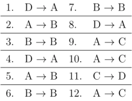
representation can be severely misleading and inacurate [10, 9, 6, 27, 28]. Consider a simple example in Table 2.1. The network representation most used is represented by the graph in Figure 2.1. To construct such a network, we identify all the nodes and then link a pair of nodes, if at least one interac-tion took place between those nodes in the entire dataset. Furthermore, we can assign weights to links, by summing the number of interactions between node pairs in the dataset.
1. D → A 7. B → B 2. A →B 8. D → A 3. B → B 9. A → C 4. D → A 10. A → C 5. A →B 11. C →D 6. B → B 12. A → C
Table 2.1: A simple example dataset of entities and their interactions.
A B C D 2 3 3 1 3
Figure 2.1: Constructed network representation for the dataset in Table 2.1. Note that the edges are weighted, according to the number of times an interaction took place between node pairs.
A random walker starting in node D, arrives to node A with P r(Xt+1 = A | Xt = D) = 1, following from the relative frequencies of outgoing link weights at node D. Continuing at node A, the random walker will choose to move to nodeB with probability 0.4 and to nodeC with probability 0.6, according to relative frequencies of outgoing link weights at nodeA. However,
6 CHAPTER 2. HIGHER-ORDER DEPENDENCIES
if we look closely at the dataset in Table 2.1, specifically at paths of length larger than one, we notice that the pattern D → A → B is predominant. The consequence of this specific pattern is the fact that the random walker is more likely to move to node B than to node C, if it has arrived to node
A from node D. The network representation in Figure 2.1 is inadequate, predicting that the random walker will most likely move to node C from nodeA, whereas in reality, this depends on how the random walker came to nodeA in the first place.
First-order networks, such as the one in Figure 2.1, work with the as-sumption that paths of length larger than one are transitive. For example, the two links in the network, (C, D) and (D, A) imply there is a relation-ship between C and A. In reality, however, whether a relationship between
C and A exists, depends on the ordering of links. Notice from Table 2.1, that the link (D, A) occurs before link (C, D), invalidating the transitivity assumption. An important observation is, that the ordering of links affects causality [27]. Traditional network construction discards ordering of interac-tions, invalidating the transitivity assumption, which most network analysis methods rely on.
Regardless of the fact that the dataset in Table 2.1 is merely a toy ex-ample, the Markov property of Markov chains implicitly modeled by tradi-tional network representations may lead to misleading results on real world datasets, as the patterns in longer node sequences are ignored and the transi-tivity assumptions invalidated. Increasing the memory of the random walker, by capturing longer sequences of past node visitations, leads to higher-order Markov chains.
2.1
Higher-order networks
Scholtes [9] presents a general framework for modeling higher-order Markov chains. Higher-order networks are most frequently used when the input is sequential data, a sequence of node visitations or, alternatively, a multi-set
of paths observed. The main idea of a higher-order network of order k > 1 is that the amount of memory a random walker stores (amount of previously visited nodes) is equal to k:
P r(Xt+1 =xt+1 |Xt=xt, Xt−1 =xt−1, . . . , X0 =x0) = P r(Xt+1 =xt+1 |Xt=xt, . . . , Xt−k+1 =xt−k+1)
(2.2)
Each node in a higher-order graphG(k)is a higher-order state node, which containskpreviously visited locations. Links between such higher-order state nodes denote a shift of node visitation history by one node forward. Let us look at an example of higher-order network construction fork= 2, given the following multi-set S of paths:
S ={(D → A → B → B), (D → A → B → B → B),
(D → A → C), (A → C → D), (A → C) }
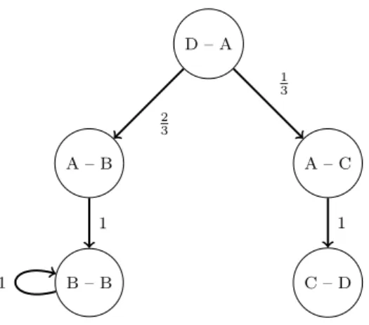
Nodes in G(2) correspond to paths of length one, in contrast to a tra-ditional first-order network, where nodes correspond to single vertices (al-ternatively paths of length zero). Identifying all distinct subpaths of length one given paths in S yields our set of nodes in G(2). Adding links between successive subpaths of length one, yields our set of interactions. Again, the transition probabilities can be approximated using relative frequencies of outgoing links at a specific node. For example, P r(B | D, A) = 2
3 as there are exactly two paths (D → A → B), while in total there are three paths (D → A → x), where x is any location. The resulting network represented by graph G(2) is visible in Figure 2.2.
8 CHAPTER 2. HIGHER-ORDER DEPENDENCIES C – D A – C D – A A – B B – B 1 1 3 2 3 1 1
Figure 2.2: A order network represented by a graph with higher-order nodes. Each higher-higher-order node is a memory node with memory size of k = 2. Links between higher-order nodes indicate shifts in observation history by one node forward.
The traditional first-order networks are simply a special case of construct-ing a higher-order network by settconstruct-ing k = 1, obtaining graph from Figure 2.1. Furthermore, the dataset in Table 2.1 can be obtained by extracting all subpaths of length one from our multi-set of pathsS.
It is important to note the distinction between state or memory nodes and actual locations. For instance, in Figure 2.2, node A− B is a state node, indicating that the random walker arrived to locationB from location
A. The actual location associated with state node A− B is therefore B. Every location may have multiple associated state nodes, e.g. location B is associated with state nodes A−B and B −B. While first-order networks capture topological dimension of the data, as every node corresponds to an actual location, the higher-order networks capture correlations in larger sequences of paths, modeling the dynamics that occur in a network [9].
2.2
Variable-order networks
How do we choose k, the amount of memory of the higher-order network, so that the representation of the underlying dynamic processes is accurate, while keeping the complexity of our model low? It is well known that a higher-order model with order k may underfit the data, while a higher-order model with order k+ 1 may already overfit the data [6]. As a result, a lot of research is conducted on the so-called variable-order networks, where a single model can contain state nodes with variable memory up to a maximum memory ofK. This allows for more flexibility in modeling the dynamic processes, increasing accuracy of the model, while keeping the degrees of freedom of a model relatively manageable. Higher-order Markov chains suffer from the curse of dimensionality as, according to Perssonet al. [6], their number of parameters requires exponentially increasing sizes of data to prevent overfitting. For a
k-th order model, the adjacency matrix of a higher-order directed graphG(k)
contains |V|k+1 transition probabilities which need to be estimated, where
V is the set of locations (paths of length zero, ordinary nodes). Because the rows of such adjacency matrix need to sum to one, the total number of free parameters is |V|k+1 − |V| (we can obtain the final transition probabilities by subtracting the rest from one). This follows from the fact that only the transitions which shift the observation history forward by one location are allowed.
There exist several approaches for constructing a variable-order network. For example, Scholtes [9] defines a so-called multi-order model MK, which consists of individual higher-order models of orders k = 0,1, . . . , K. The probability of generating a path (v0 → . . . → vl) with the model MK is defined as the product of transition probabilities of subpaths with increasing orderk = 0,1, . . . , K, while also taking into account that the length of path
l may be larger than the maximum order of the model K. For instance, the probability ofM3 generating the path (a→b →c→d→e) is equal to:
10 CHAPTER 2. HIGHER-ORDER DEPENDENCIES
P r(a, b, c, d, e) = P r(a)· P r(b |a)·P r(c|a, b)· P r(d|a, b, c)·P r(e|b, c, d)
(2.3)
A model of order k = 0 can be viewed upon as specifying prior prob-abilities of the random walker starting it’s walk in each of the locations. Scholtes then suggests a likelihood ratio optimization procedure to deter-mine the optimal K value of a multi-order model MK. First, a likelihood function L(MK | S) is defined based on the product of probabilities of all paths in S. Then, choosing a model MK+1 in favor of a simpler model MK depends on whether the likelihood of the former is significantly higher than the likelihood of the latter model. As soon as this is no longer the case, the optimal order Kopt has been found.
Xuet al. [10] provide an even more compact representation of a variable-order Markov chain by storing in the variable-variable-order network only the state nodes corresponding to higher-order correlations found in the data, rather than considering all possible transition probabilities between higher-order nodes. Using their approach, the parameter explosion resulting from|V|k+1− |V| transition probabilities is eliminated, as only the statistically significant higher-order correlations are considered. Their variable-order construction algorithm bears some similarity to the Apriori algorithm [29], used for mining frequent item sets. In the first stage of their algorithm, a set of rules corre-sponding to higher-order patterns is extracted from the sequential data. The algorithm starts out with first-order dependencies (paths of length one) and then attempts to extend them to higher correlation orders, up to a maximum orderK. If the memory increase of a state node significantly alters outgoing transition probabilities compared to the outgoing probability distribution of the original state node, a higher-order rule is justified. The minimum rule support parameter allows the authors to control the compactness of the re-sulting variable-order network and to prevent overfitting. A low minimum support allows the algorithm to identify a large set of rules, even if the rules are insignificant, fitting the model to noise in the data. A higher minimum
support identifies only rules that occur frequently, preventing overfitting. In the second stage, the extracted rules are used to create a variable-order network representation, which encompasses both state/memory nodes and physical/location nodes.
Persson et al. [6] view the dynamics of the network — higher-order cor-relations — as flows of information. They start out with one state node for every location and then ”unlump” the state nodes, producing more and more state nodes for every location, according to the largest decrease in entropy rate. Once a sufficient number of state nodes is reached, links are added among these nodes. Such sparse Markov chains have a strictly decreasing entropy rate with increasing numbers of higher-order nodes. An optimal Markov chain is selected using model selection techniques.
2.3
Temporal dimension
As we have seen in the previous sections, dynamic processes on a network are based on the ordering of interactions between entities. However, the dynamic processes evolve at certain time scales, which are usually much shorter than the observation period, during which the dataset was sampled [9]. Addi-tional temporal dimension, which assigns timing information to interactions, can alter the ordering of these interactions, causing different higher-order cor-relations. Scholtes et al. provide an in-depth overview of temporal networks [27], which we summarize here. In a temporal network, each interaction is a tuple (A, B, t), whereAand B are entities in interaction, whilet ∈[0, T] is a discrete timestamp denoting the time at which the interaction took place. A
time-respecting pathis a sequence of interactions, with increasing timestamps,
i.e. (A, B, t1), (B, C, t2), (C, D, t3), . . . , (X, Z, tn); t1 ≤t2 ≤ · · · ≤tn. The requirement of increasing timestamps causes an ordering of the links, one that may be different from the implicit ordering provided by sequential order of interactions in the dataset. Scholtes [9] in his later work demonstrates, that the temporal dimension merely affects the ordering of the interactions
12 CHAPTER 2. HIGHER-ORDER DEPENDENCIES
and that no change is required to the higher-order Markov chain framework. The input is still a multi-set of paths, albeit with a different ordering of nodes in paths, due to timestamps.
However, the timing information of interactions allows us to observe dy-namic processes at different time scales. This can be achieved through the notion of maximum time difference δfor respecting paths [27]. A time-respecting path (vo, v1, t1), . . . , (vl−1, vl, tl) conforms to a maximum time difference δ if and only if 0 < ti+1−ti ≤ δ, i = 0, . . . , l. In other words, a time-respecting path with maximum time differenceδ consists of only inter-actions that are maximumδ time apart. Choosingδ is equivalent to filtering out paths in the multi-set of paths S. A small value of δ will only keep the paths that capture dynamic processes at small time scales, while choosing a large value ofδwill filter less, preserving most of the paths found in the data, including those that occur over large periods of time. The optimal choice of value for δ is a difficult problem in itself. Scholtes suggests approximating δ
using inter-interaction time distribution [9].
The following set of timestamped interactions better demonstrates the role of δ parameter:
A−→1 C, C −→2 E, B −→4 C, C −→5 D, B −→7 C, C −15→E
Using δ = 1 filters out the paths A −→1 C −→5 D and B −→7 C −15→E, using
δ = 4 filters out only the path B −→7 C −15→ E, while using δ = ∞ preserves all the paths.
A more subtle approach to encoding temporal information is by consid-ering conditional waiting times, proposed by Matamalas et al. [28]. Take for instance a path A →A → A → B →B → B → B. The variable-order Markov models in the previous sections fail to account for the amount of time spent in every physical location node. One of the reasons for this is that the higher-order rules that would capture such patterns have insufficient support and are pruned. Other reasons include an insufficient maximum allowed memory size K of a model. A common solution is to reduce the sequence of
node visitations to unique entries only, i.e. to convert the above path into
A→B. This however discards the temporal information implicitly provided by the number of successive location nodes.
The conditional waiting time of a node encodes additional information on how long is a random walker likely to spend at a particular location, given the previous steps the walker took. This is important in domains such as disease spreading or information diffusion. Failing to account for conditional waiting times could lead to poor predictions on the speed of diffusion processes occurring in the network [28].
Matamalaset al. propose a solution to this problem calledadaptive mem-ory. The core idea of this approach is to allow additional entries in the full transition matrix of a higher-order Markov chain, while generating subpaths by skipping successive nodes corresponding to the same location. It is best to take a look at an example. Taking the path A → A → A → B → B → B → B and a fixed-order Markov model with k = 2, the adaptive memory approach would generate the following subpaths, which are later converted to higher-order nodes: A→A→A, A→A→B, A→B →B, A@ @ B →B →B, A@B@@@B →B →B
Because of the limited memory of k = 2, previous location A would have been lost upon reaching the subpath B → B → B → B. Forcing the previous location to remain as the first node in the higher-order pattern allows for better predictions, while the conditional waiting time is reflected in the cardinality of the pattern, namely pattern A → B → B which now occurs three times in total.
14 CHAPTER 2. HIGHER-ORDER DEPENDENCIES
In terms of transition matrices, the above approach allows for additional transitions not allowed in higher-order Markov chains. A transition of (A− B)→(A−B) for example is not allowed in the transition matrix of a higher-order Markov chain, as the node visitation history is not shifted by one node forward, while this is perfectly acceptable in adaptive memory approach.
Significant pattern detection
Chapter 2 revealed that in general, modeling higher-order dependencies of increasing order results in a combinatorial explosion. Withn= 10 first-order nodes (physical locations), there are 102 = 100 possible second-order rules, 103 = 1000 third-order rules, etc., describing the dynamics of a network. To mitigate the issue, variable-order models are used which encode higher-order dependencies of various orders, specifically those found in the data. However, even a variable-order model encodes a substantial amount of higher-order patterns as it captures both the noise in the data and the important patterns. In order to obtain interesting information from the data, we desire to filter out higher-order dependencies and find only the statistically significant ones. This enables us to observe which node visitation histories significantly affect the transitions of the random walker. We seek a way to sort higher-order patterns according to their importance.
The variable-order model proposed by Scholtes [9] does not allow for in-dividual higher-order rule discovery, but tests the whole model Mk+1 versus Mk. Such approach gives limited information on which specific higher-order rules are significant, i.e. not produced by noise in the data. A good initial proposal is that of Xu et al. [10], who use the Kullback-Leibler divergence measure [30] to detect significant deviations in the outgoing probability distri-butions caused by increased history size. Every state node in a variable-order
16 CHAPTER 3. SIGNIFICANT PATTERN DETECTION
network has an outgoing probability distribution associated with it, as the next location depends on the transition probabilities given the current his-tory. For instance, the state nodeA−B−C may have the following outgoing probability distributionp:
(A−B −C)→A: 0.12 (A−B−C)→C : 0.49 (A−B −C)→D: 0.39
Xuet al. detect significant higher-order patterns by increasing the history size of a specific pattern, then measuring whether there is a significant change in the outgoing probability distributions, comparing the previous and the new distributions. Increasing the history of pattern (A, B, C),e.g. could alter the transition probabilities, producing the altered probability distribution q:
(D−A−B−C)→A: 0.11 (D−A−B −C)→C : 0.33 (D−A−B−C)→D: 0.56
The Kullback-Leibler divergenceDKL(p, q) measures the expected loss of information when approximating probability distributionpwith distribution
qand is defined as the expectation of the log difference between probabilities of two discrete distributions:
DKL(p, q) = X i p(xi)·log p(xi) q(xi)
Xu et al. [10] find the altered probability distribution q significant, if
DKL(p, q)>
Order(q) log2(Support(q)),
whereOrder(q) = 4 is the history size of higher-order rules, whileSupport(q) denotes the number of occurrences of a particular state node. The assump-tion of such approach is that patterns of high order are less likely, while the patterns which have high support (occur frequently in the data) are more likely.
Such approach also does not allow for individual higher-order rule testing, as entire outgoing probability distributions are compared. If, for example,
q was found to be significantly different than p, then all the higher-order rules in q would be deemed significant, even though it is clear that pattern (D−A−B −C−A) is not significant since adding node D does not alter the transition probability much (0.12 versus 0.11).
Instead we use a different procedure, which relies on hypothesis testing. We use the variable-order modelMK proposed by Scholtes [9], which encodes all higher-order patterns up to maximum order K. The probability of MK generating a specific pattern generalizes from example (2.3), but we skip the prior probability of a random walker starting in specific node (k >0):
P r(v1, v2, . . . , vl) = P r(v2 |v1)·P r(v3 |v1, v2)·. . .·P r(vi |vi−K+1, . . . , vi−1) ·P r(vi+1 |vi−K+2, . . . , vi)·. . .·P r(vl |vl−K+1, . . . , vl−1) (3.1)
The intuition behind our approach is that if a higher-order pattern (v0, v1, . . . , vK) of order K is significant, then it should be predicted well by the model MK
(pattern is in accordance with the model), but predicted poorly by a model which uses less history, MK−1. If the pattern is predicted poorly by both MK and MK−1 then this is a result of either an anomaly in the data, inad-equate amount of training data for our model or the result of limitations in the model itself.
In order to test how well is a pattern predicted by the model MK, we use hypothesis testing procedure. Assume again a pattern (v0, v1, . . . , vK) of length K for simplicity. The model MK outputs the total probability pm of generating this pattern, according to equation (3.1). The resulting value
18 CHAPTER 3. SIGNIFICANT PATTERN DETECTION
states the probability of obtaining this pattern, if a random walk starting in node v0 of length exactly K was made in a traditional, first-order network. The length of the random walk denotes the amount of visited locations in the first-order network including v0. In comparison with the model, we also have an empirical value for probability of the pattern. Let rdenote the total number occurrences of pattern (v0, v1, . . . , vK) and let n denote the total number of subpaths of size K starting in v0. The empirical probability is simply a relative frequency pe= rn, according to the data.
How well a model predicts the pattern depends on how similar are both probabilities pm and pe. Because consecutive random walks in the network are independent, the total number of occurrences of (v0, v1, . . . , vK) follows a binomial distribution with parameters pm and n. We use a two-tailed binomial test to assert whether pm deviates significantly from pe:
H0 :pe =pm
H1 :pe 6=pm
Rejecting the null hypothesis tells us that the pattern cannot be predicted well by MK. Using a two-tailed test allows us to check if a pattern is either over- or under-represented in MK. Because with large values of parameter
n the binomial test breaks down due to increasing complexity of having to calculate the cumulative distribution function involving factorials, we replace the binomial test with a two-tailed z-test, i.e. we approximate the binomial distribution with the standard normal distribution. This follows from the central limit theorem, as the normal approximation is accurate for large values of n. The test statistic becomes:
z = p |pe−pm| ˆ p(1−pˆ)·2/n (3.2) where ˆ p= n·pe+n·pm 2n = pe+pm 2 (3.3)
The p-value is then calculated as 1−ncdf(z) +ncdf(−z), where ncdf
is the standard normal cumulative distribution function. We reject the null hypothesis H0 if p-value is below a specified significance threshold α. The entire procedure can be iteratively expanded to test patterns of increasing order K, while the model MK is updated with significant patterns as we proceed.
Algorithm 1 Significant pattern detection algorithm
Require: multiset of paths S, maximum orderK, significance thresholdα Ensure: list of significant patterns
initialize rules to an empty array
for k= 2 toK do
Sk= all subpaths of length k fromS
for all (v0, v1, . . . , vk)∈Sk do
r = total number of occurrences of (v0, v1, . . . , vk)
n = total number ofp∈Sk, which start with v0 pe = nr
pMk = probability of (v1, v2, . . . , vk) according to Mk pMk−1 = probability of (v1, v2, . . . , vk) according to Mk−1
zk=ztest(pe, pMk, n) according to (3.2) zk−1 =ztest(pe, pMk−1, n) according to (3.2)
if p-value of zk−1 ≤α and p-value of zk > αthen add ((v0, v1, . . . , vk), p-value of zk−1) to rules array end if
end for end for
sort rules according to increasingp-values
return rules
Algorithm 1 has an added advantage of returning a sorted list of signif-icant patterns according to increasing p-values. The lower the p-value, the more certain we are in rejectingH0 and accepting a pattern as significant.
20 CHAPTER 3. SIGNIFICANT PATTERN DETECTION
3.1
Artificial data
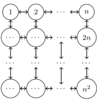
We now test the procedure described in Algorithm 1 on generated, artificial trajectories. We use a simple directed graph represented by a square n×n
grid as the basis for the random walks, which generate the trajectories to be used as input.
1 2 . . . n
. . . 2n
. . . .
. . . n2
Figure 3.1: A directed graph represented by a squaren×n grid.
We use the directed graph presented in Figure 3.1 to perform 10 000 random walks, each of length K + 10, based on a model giving transition probabilities. With the model we can define a set of higher-order dependen-cies by altering the transition probabilities based on specific history of visited nodes.
We focus first on n = 2, i.e. a 2×2 square grid, and use a model with two second-order dependencies, with no other higher-order dependencies, as visible in (3.4).
1 2
3 4
1→2 : 0.5 1→3 : 0.5 2→1 : 0.5 2→4 : 0.5 3→1 : 0.5 3→4 : 0.5 4→2 : 0.5 4→3 : 0.5 (2,1)→2 : 0.1 (2,1)→3 : 0.9 (4,2)→1 : 0.1 (4,2)→4 : 0.9 (3.4)
Table 3.1 shows the returned significant patterns by running Algorithm 1. The results are based on a search for up to fifth order patterns (K = 5). As it is clearly seen, the algorithm correctly identified that there are no patterns of order higher than two. Furthermore, the second-order patterns (4,2,1) and (2,1,2), which are under-represented in the model (3.4), have the lowest
p-value, while the patterns which are over-represented in the model, (2,1,3) and (4,2,4), are also in the list of significant patterns.
It is interesting to explore why did the model find patterns (1,2,1) and (1,2,4) significant, as they were not specifically encoded in the model (3.4). If we break up the patterns into the probability product predicted by the model M1 (according to equation (3.1)), we find the following probabilities: P r(1,2,1) = P r(2 | 1)·P r(1 | 2) and P r(1,2,4) = P r(2 | 1)·P r(4 | 2). From model (3.4), we find that P r(1 | 2) = 0.5. However, in the empirical probabilities calculated from the generated trajectories, we find that P r(1 |
2) = 0.4, causing a difference in probabilities, a lowp-value and therefore the rule is marked as significant. The reason for such deviation from the model is the higher-order dependency rule (2,1) → 2 : 0.1 encoded in the model, which causes the random walker to use the first-order connection 1 → 2 much less than it normally would. It is apparent that higher-order rules affect lower-order rules as well.
22 CHAPTER 3. SIGNIFICANT PATTERN DETECTION Pattern p-value (4,2,1) 1.01·10−282 (2,1,2) 7.75·10−261 (1,2,1) 8.17·10−166 (1,2,4) 1.40·10−117 (2,1,3) 2.42·10−109 (4,2,4) 4.89·10−100 (3,1,2) 1.84·10−58 (3,1,3) 3.61·10−51
Table 3.1: A list of significant patterns and their p-values, returned by Algorithm 1, with K = 5, α = 0.01 and 10 000 generated trajectories based on model (3.4) and a 2×2 grid from Figure 3.2.
We now look at a second example, a model with a single fifth-order de-pendency, as given in (3.5), with the same 2×2 grid as in Figure 3.2. Table 3.2 shows howp-values of pattern are increasing with increasing history size, as anticipated. Model M1 has the lowest p-value as it has the lowest his-tory size and is unable to account for higher-order correlations. Model M4 still falls short of the α = 0.01 significance level, as the lack of fifth node in observation history critically affects the transition probabilities.
1→2 : 0.5 1→3 : 0.5 2→1 : 0.5 2→4 : 0.5 3→1 : 0.5 3→4 : 0.5 4→2 : 0.5 4→3 : 0.5 (3,1,3,1,2)→1 : 0.1 (3,1,3,1,2)→4 : 0.9 (3.5)
From this example it is evident that higher-order dependencies affect the significance of lower-order dependencies as well. Algorithm 1 finds patterns (1,3,1,2,4), (3,1,2,4) and (1,2,4) significant in addition to the fifth-order pattern (3,1,3,1,2,4). Notice how the lower-order patterns are suffixes of the original fifth-order pattern. The reason for lower-order patterns being
significant in addition to the fifth-order pattern is the final transition 2→4, which has an extreme transition probability of 0.9 according to the model (3.5), in the fifth-order rule. This extreme probability affects the transitions of the random walker and because all suffixes of the pattern (3,1,3,1,2,4) also take into account the transition 2→4, they are found significant. If, for instance, we change the transition probabilities of the model (3.5), so that (3,1,3,1,2)→1 : 0.3 and (3,1,3,1,2)→4 : 0.7, Algorithm 1 no longer finds lower-order patterns (3,1,2,4) and (1,2,4) significant, because the fifth-order dependency no longer has a drastic effect.
Model p-value of (3,1,3,1,2,4) M1 4.81·10−39 M2 6.12·10−34 M3 8.89·10−28 M4 1.68·10−13 M5 0.9588
Table 3.2: The increasing p-values of models with increasing memory size, up to the size of pattern, K = 5. Based on model (3.5) and a 2×2 square grid from Figure 3.2.
3.2
Anomaly detection
The procedure described in Algorithm 1 can be looked upon as the training phase, in which we fit a variable-order modelMK of maximum orderK to the trajectory data. The added bonus of the training phase is the identification of higher-order patterns that significantly affect the transition probabilities. But what if we are given a new set of trajectories, namely a testing set of data and are asked what patterns are poorly predicted by the current model
MK? Such questions are common in anomaly detection, where a model is first trained on a large set of training data, to capture the most common traffic patterns, and is then given an alternative data which may contain
24 CHAPTER 3. SIGNIFICANT PATTERN DETECTION
patterns of different frequencies, resulting in an anomaly.
The anomaly detection procedure is quite simple and similar to that of Algorithm 1. We again perform statistical testing if the empirical probability of specific pattern deviates significantly from probability predicted by the model, which in-turn depends on the training phase. The entire procedure is summarized in Algorithm 2.
Algorithm 2 Anomaly detection algorithm
Require: testing set of paths Stest, model MK from the training phase, significance threshold α
Ensure: list of significant patterns, i.e. anomalies initialize anomaliesto an empty array
for k = 2 to K do
Sk = all subpaths of lengthk fromStest
for all (v0, v1, . . . , vk)∈Sk do
r= total number of occurrences of (v0, v1, . . . , vk)
n= total number ofp∈Sk, which start with v0 pe = nr
pMK = probability of (v1, v2, . . . , vk) according to MK z =ztest(pe, pMK, n) according to (3.2)
if p-value of z ≤α then
add ((v0, v1, . . . , vk), p-value of z) to anomalies array
end if end for end for
sort anomaliesaccording to increasing p-values
return anomalies
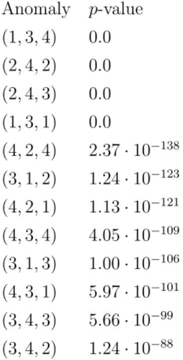
We perform an experiment on two different models giving transition prob-abilities for the random walker on a 2×2 grid from Figure 3.2. The first model encodes a second-order rule of (2,4) → 2 : 0.1 and (2,4) → 3 : 0.9, while the second model encodes a second-order rule of (1,3) → 1 : 0.1 and
(1,3)→4 : 0.9. We use both models to produce 10 000 trajectories of size 12 each. We use the first 10 000 trajectories from the first model as the training set and the second 10 000 trajectories from the second model as the testing set. Anomaly p-value (1,3,4) 0.0 (2,4,2) 0.0 (2,4,3) 0.0 (1,3,1) 0.0 (4,2,4) 2.37·10−138 (3,1,2) 1.24·10−123 (4,2,1) 1.13·10−121 (4,3,4) 4.05·10−109 (3,1,3) 1.00·10−106 (4,3,1) 5.97·10−101 (3,4,3) 5.66·10−99 (3,4,2) 1.24·10−88
Table 3.3: A list of anomalies and their p-values, returned by Algorithm 2, with K = 2 andα = 0.01.
Table 3.3 displays the resulting anomalies found by Algorithm 2. As ex-pected, patterns (1,3,4) and (1,3,1) are anomalies because they are encoded in the second model used to generate testing data, while patterns (2,4,2) and (2,4,3) are also anomalies because they are not encoded in the second model producing the testing data, but were present in the first model producing the training data. Other anomalies are the direct result of the first four anoma-lies, as the second-order patterns affect transition probabilities of first-order patterns as well.
When using the training data as the testing data, no anomalies are found, which is in accordance with our expectations.
Chapter 4
Computer communication
networks
Chapter 2 and Chapter 3 have defined higher-order dependencies, gave us a way to find important dynamics in the vast datasets and are in theory ready to be applied to any desirable sequence-like data for which we seek to understand dynamics. However, in practice, we are often faced with addi-tional problems such as noisy data, missing values, too much data or the the dataset does not exhibit higher-order correlations at all. Before we dive into computer network traces, it is vital to understand what we can expect from such datasets. In this chapter, we review the basics behind the two most used networking protocols to this day, and give an overview of the type of dynamics that arise from computer communications.
Our choice of domain are computer networks, more specifically the packet traces in the transport and application layers of the TCP/IP model. We fo-cus on segments from the two most used protocols in the transport layer, the Transfer Control Protocol (TCP) and the User Datagram Protocol (UDP). Regardless of the protocol, the transport layer encapsulates traffic from the application layer and provides a logical communication link between two endpoints in a network. The link is termed logical because the underlying network structure and topology, consisting of routers, switches and links, is
abstracted away. Both endpoints communicate as if they were connected di-rectly, ignoring the details of the lower network layers in the TCP/IP model. The fundamental task of the transport layer is to extend the host-to-host communication, which the network layer (along with the IP protocol) pro-vides, to process-to-process communication of the processes running on in-dividual hosts [31]. An additional task of the transport layer protocols is to perform multiplexing and demultiplexing operations, forwarding messages from a single network interface to different processes and vice-versa. This is achieved through the use of a 16-bit identifier called port or socket number, assigned to each of the running processes. The first 1024 port numbers are reserved and termed well-known port numbers. Although all transport layer data traces contain only TCP and UDP segments, it is possible to determine the application layer protocol encapsulated in the segment simply by observ-ing well-known port numbers. For instance, the port number 80 corresponds to the HTTP protocol. With port numbers larger than 1023 the application layer protocol can no longer be reliably determined.
Whereas the transport layer provides a logical communication link be-tween processes running on individual hosts, the network layer provides a logical communication link between individual hosts in the global network structure, abstracting away the switches and physical links that connect the hosts. The IP protocol, which assigns a unique 32-bit identifier to each host termed the IP number (for simplicity, we focus specifically on the IPv4 proto-col), allows for addressing of devices in the network structure (either local or global). Thus, a network trace that is captured at one of the hosts in the net-work is expected to have at least the following attributes: source IP address, source port number, destination IP address and destination port number. The source identifiers are necessary for bidirectional communication.
Figure 4.1 depicts the complexity that naturally arises from the layered architecture of computer communication networks. There are several vari-ables to consider for a network trace dataset, before attempting to use net-work analysis and higher-order methods. From the netnet-work layer
perspec-28 CHAPTER 4. COMPUTER COMMUNICATION NETWORKS
tive, an important consideration is where the tracing program was placed,
i.e. on which host (IP address). For example, we can monitor the intra-network communication (communication between hosts123.218.44.78and
123.218.44.209 in Figure 4.1), the inter-network communication
(commu-nication between hosts 123.281.44.5 and 46.164.13.66 in Figure 4.1) or both. Most datasets we have tested are the result of a trace being run on the edge router between the sub-network and the rest of the Internet (inter-network communication). Such traces are also the most interesting, as the majority of application protocols run across the Internet rather than in sub-networks (e-mail and web pages). Such traces also make the most sense, as network attacks most frequently originate from outside the sub-network.
Figure 4.1: An example of a computer network architecture, depicting the process-to-process communication, while also outlining the significance of IP addresses. The sub-network uses public IP addresses, ignoring details such as network address translation (NAT), to keep complexity to a minimum.
A second variable to consider is how to interpret the network trace data from the network analysis standpoint, i.e. what would be the nodes in the network and what the relations between those nodes. We found the follow-ing interpretation satisfactory. A node corresponds to a particular packet destination in the dataset. Clients, or packet sources in the dataset, per-form a walk in the network of such nodes, producing trajectories of packet destinations (clients repeatedly choose different packet destinations to send packets to). Two nodes are connected or in a relation, if any client used them in succession (in a traditional, first-order network). The definition of a node is intentionally vague, because a packet destination can be defined in multiple ways. The simplest approach is to treat all destination IP addresses as packet destinations and therefore nodes. Another approach is to use port numbers, and thereby application layer protocols, as packet destinations, or a combination of both. As the majority of publicly available datasets use some form of IP address anonymization procedure and because the IP ad-dress itself gives almost no valuable information on the type of traffic, we decided to focus on port numbers and protocols instead. Using a combina-tion of IP address and destinacombina-tion port is also an opcombina-tion, but is problematic, because there is little overlap in the destination IPs used by different clients. Clients are likely to use their own set of destination IP addresses that does not overlap with other clients, e.g. every website is hosted on a web server with it’s own IP address and every client is more likely to browse it’s own unique set of web sites. Even a single website can have multiple associated IP addresses to help with load balancing. Completely disregarding IP addresses however, is also not an option, because they do provide one important piece of information. Observing two consecutive connections of one client allows us to detect whether a destination host has changed or remained the same. In our final implementation, we use the information from two consecutive IP address identifiers and append it to the protocol/port number identifier. If a protocol was used on the same host it is marked asprotocol*, while if the destination IP address was changed, no* identifier is present.
30 CHAPTER 4. COMPUTER COMMUNICATION NETWORKS
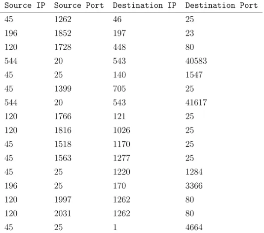
To better illustrate our choice of node and relation interpretation, con-sider the following example dataset in Table 4.1, which is a subset of TCP traffic trace between the Lawrence Berkeley Laboratory and the rest of the world [32]. In this example, packet sources or clients can be either theSource IPidenfitier or a combination of(Source IP, Source port)identifiers. We have found the Source IPidentifier as the packet source to be adequate, as otherwise the trajectories are broken up into much smaller paths. The packet sources themselves are merely random walkers and are not translated into a network representation.
Source IP Source Port Destination IP Destination Port
45 1262 46 25 196 1852 197 23 120 1728 448 80 544 20 543 40583 45 25 140 1547 45 1399 705 25 544 20 543 41617 120 1766 121 25 120 1816 1026 25 45 1518 1170 25 45 1563 1277 25 45 25 1220 1284 196 25 170 3366 120 1997 1262 80 120 2031 1262 80 45 25 1 4664
Table 4.1: An example network trace dataset to illustrate different possible interpretations of nodes and edges from a network analysis standpoint. IP addresses have been anonymized and replaced with integer identifiers.
Like previously mentioned, there are several options for packet destina-tions or nodes in the first-order network. We group the dataset in Table 4.1 according to the packet source (Source IP column) and convert the packet destinations of every packet source into a sequence-like data or trajectories. The ordering of individual packet destinations within each trajectory depends on the original ordering in the dataset, which may be arbitrarily changed by permuting the rows of the dataset (or by sorting the dataset based on a timestamp column). For example, the following trajectories are obtained if we chooseDestination port as our packet destination:
45: 25, 1547, 25, 25, 25, 1284, 4664 196: 23, 3366
120: 80, 25, 25, 80, 80 544: 40583, 41617
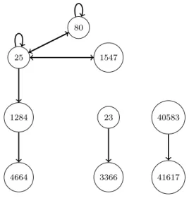
The trajectories can then be used to produce first-order and higher-order graphs as well. An example of first-order graph is visible in Figure 4.2.
25 1284 4664 80 1547 23 3366 40583 41617
Figure 4.2: A first-order network constructed from example dataset in Table 4.1 by using Destination portas packet destination.
destina-32 CHAPTER 4. COMPUTER COMMUNICATION NETWORKS
tion leads to loss of information. Specifically, the sub-sequence 25, 80, 80
of packet source 120, corresponding to repeated use of HTTP protocol, does not reveal if the protocol was used to communicate with one host or with different hosts. By also taking into account theDestination IPcolumn, an alternative set of trajectories is obtained, one that allows us to observe if the hosts have changed (* marks same hosts):
45: 25, 1547, 25, 25, 25, 1284, 4664 196: 23, 3366
120: 80, 25, 25, 80, 80* 544: 40583, 41617*
Rarely are we provided with a ready-to-use dataset such as the one in Table 4.1. TCP protocol, for instance, segments the data and sends it in chunks during a single session. Furthermore, every received segment must be acknowledged, resulting in an overflow of packets that have to be analyzed. As a result, raw TCP trace data contains all packets, both those used to ini-tiate a session and those used during the session. We are of course interested only in successive protocols being used, so we keep only the packets related to session initiation. UDP protocol has no such issue, as it sends the data as-is (the application layer has to take care of segmentation). Specific quirks in the application layer protocols are captured as dynamics, represented by higher-order correlation. For instance, in Figure 4.1, clients 123.218.44.78
and 123.218.44.209 communicate using FTP protocol’s active mode, but
this is well captured by modeling dynamics, removing the need to handle such edge cases manually.
Last but not least, we have to consider that the type of communication network may not exhibit higher-order correlations at all. Such was the case when we used our significance detection framework on anonymized internet traces from CAIDA’s equinix-chicago monitor on high-speed Internet back-bone links [11]. As the transport layer protocols are point-to-point logical connections and because we opted for a network representation using destina-tion port numbers as nodes, the presence of recurring paths of length larger
than one depends not only on where the traffic monitor is placed, but also on how much overlap there is among different trajectories of packet sources. In the case of CAIDA, the traffic monitor was placed on a high-speed backbone link, causing not only an enormous amount of traffic, but also the type of traffic was mostly forwarded packets. This resulted in an insignificant over-lap between trajectories of different packet sources and consequentially no order correlations. If we are to have any hope of detecting higher-order correlations in computer communication networks, we should focus on consumer sub-networks, rather than on key architectural endpoints in the global internet structure.
Chapter 5
Results
Chapter 4 outlined the type of datasets we are looking for within the do-main of computer communication networks. We are interested in TCP and UDP packet traces of consumer-oriented networks and we are looking for data traces which were taken at a border router of the sub-network. We first present our results of higher-order network analysis on a TCP trace provided by Paxson [12]. The dataset contains a wide-area monthly trace of all TCP packets between the Lawrence Berkeley Laboratory and the rest of the world. The tracing program ran between September 16, 1993 through October 15, 1993. The dataset is quite old and not really representative of the current dynamics in the global Internet structure. Back in 1993, internet commu-nication was not yet widely spread and security did not yet pose an issue. Consequentially, a lot of insecure protocols such as Telnet were widely used, while more modern and secure protocols such as SSH were just emerging. A lot of old protocols found in this dataset are nowadays obsolete, such as the old Line Printer Daemon (LPD) protocol that was replaced by the Internet Printing protocol (IPP) or the Gopher protocol superseded by the HTTP protocol. Nonetheless, it is useful to analyze the significant higher-order patterns found by our framework, as we know what to expect in terms of dynamics for every protocol. However, in order to understand the dynamics found by our framework, we first require specific knowledge of the domain.
We therefore give a brief overview of the most used protocols of pre 2000 era in Table 5.1.
Protocol (associated ports) Description
Telnet [33] (23) Remote terminal access. Used to connect to mote hosts and run command line commands re-motely. Uses no encryption by default.
X window system (6000-6063) Remote graphical user interface protocol. A server controls the hardware (display, keyboard, mouse), while clients connect to the server and issue graphical commands such as displaying a window, drawing on screen etc.
Finger [34] (79) Provides status report and user information shar-ing of remote systems. The protocol was primar-ily used to check online status of people on re-mote machines and to exchange simple informa-tion such as name and e-mail addresses.
Remote login [35] (513) Almost equal to Telnet protocol, allows users re-mote terminal access. Unlike with Telnet, the server can specify a list of trusted clients and those clients require no authentication.
Internet Relay Chat [36] (194, 6667) Text chat based on client-server architecture. A group of clients connect to a chat server to ex-change text messages.
Gopher [37] (70) Known as the predecessor of the modern web, it provided online access to documents using a hi-erarchical directory structure.
Table 5.1: An overview of the most frequently used application-layer proto-cols before the year 2000, as observed in Lawrence Berkeley traces [12]. Note that all of the protocols use TCP as the underlying transport-layer protocol. Some of these protocols are still widely used today.
36 CHAPTER 5. RESULTS
5.1
Berkeley data set
We now provide the results of higher-order pattern detection of maximum order up to K = 5 on the Lawrence Berkeley TCP traces [12]. We list a few most interesting higher-order patterns which were found to be significant, as seen in Table 5.2.
Pattern Description
ftp, ftp-data*, ftp-data* In accordance with FTP protocol, where a control connection is established first and then the data connection takes place on the same host.
finger, smtp*, finger* Interesting because the client first used the Finger protocol to obtain information from the remote host, which is a SMTP server at the same time.
ftp, login*, ftp* The client started a FTP control session and also used remote login procedure to access the remote host.
login, login*, X11* The client first used remote login to access the remote host and then established a X11 session to run graphical programs on the remote host, most likely piggybacking over existing login session.
printer, smtp, ftp A typical example of a client using all popular services of the Internet at that time.
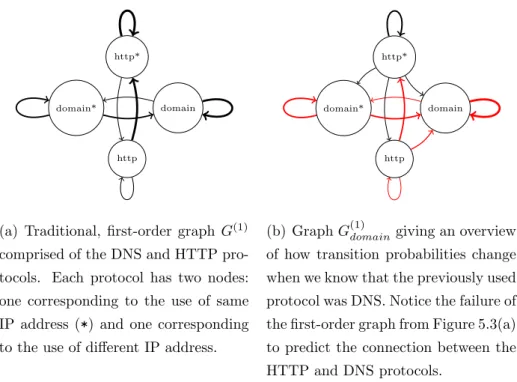
domain, domain, domain*, domain
An example of DNS query where three different
DNSservers are involved. Interesting also because DNS most usually operates using UDP as the un-derlying transfer protocol.
smtp, printer, printer*, printer*, printer*, smtp
A client which sends two e-mails and completes a print-job on one remote host.
Table 5.2: Most interesting higher-order patterns which were found sig-nificant while investigating Berkeley TCP traces [12] (α = 0.01). Protocols marked with*identifier denote that the destination IP address remained the same. The interpretation of these patterns is only hypothetical.
We also visualize the results using graphs. Because there are many pro-tocols (physical nodes) in the dataset and because each protocol has two
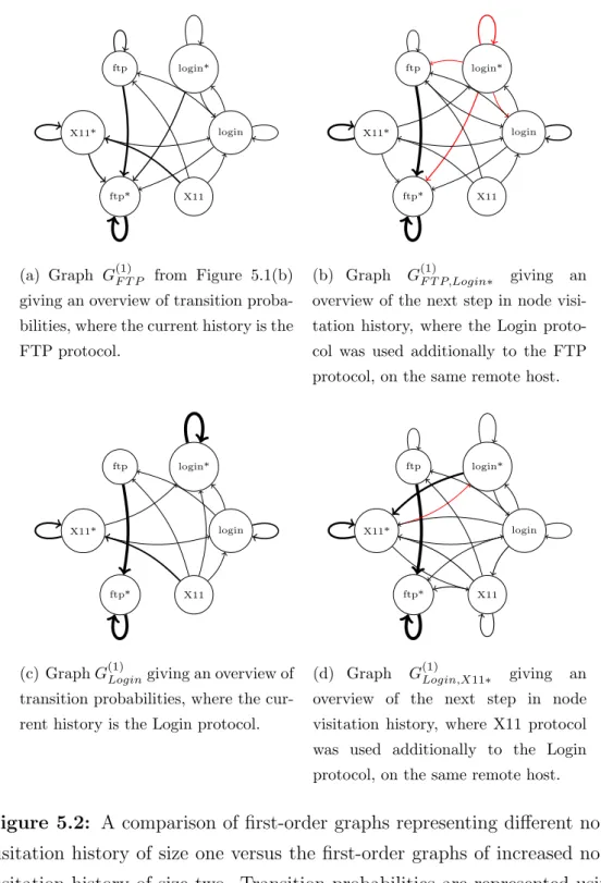
cor-responding nodes (indicating the same or different IP address), we restrict ourselves to the following protocols: FTP, X11 and Telnet/Remote login. Furthermore, we join both the FTP control and data connections (ports 20 and 21) into a single protocol and we treat Telnet and Remote login protocols as one, due to their similarities. This greatly reduces the size of graphs we are about to present (induced subgraphs of subset of nodes), while still outlines the importance of higher-order dynamics. To further reduce the complexity we opt for the following visualization technique. We visualize each higher-order graph G(k) of order k as a first-order graph. We do this by producing a set of first-order graphs, based on every history combination of sizek. The transition probabilities of these first-order graphs are determined according to the specific node visitation history which the graph represents. For exam-ple, for a second-order graph G(2) and three most used protocols, we have five first-order graphs,G(1)F T P, G(1)Login and G(1)X11, each representing transition probabilities for different node visitation histories. A third-order graph G(3)
would have eighteen first-order graphsG(1)F T P,F T P,G(1)F T P,F T P∗,G(1)F T P,Login etc. Protocols used on the same remote host, i.e. marked with*, are not allowed as the first element in node visitation history. Because the number of differ-ent node visitation history combinations rises expondiffer-entially with increasing order k, we keep only those first-order graphs, which contain a significant higher-order pattern found in the previous step.
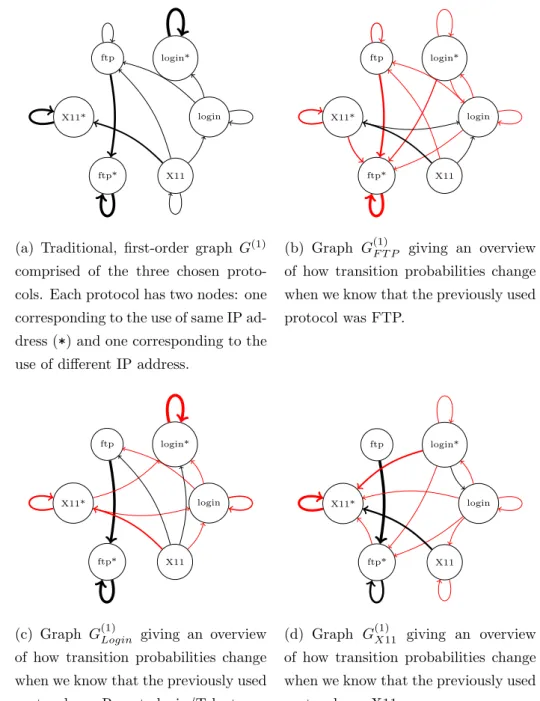
Figure 5.1 provides an overview of how dynamics change with the second-order dependencies in comparison with the traditional first-second-order dynamics. Graph in Figure 5.1(b) demonstrates how knowing that the previous used protocol was FTP results in all transitions converging back to the FTP pro-tocol, but on the same remote host (IP address). The packet source is much more likely to use the FTP protocol again, coming from the Login and X11 protocols and, is now less likely to remain in these protocols (reduced weights on self-loops). Furthermore, you are now more likely to remain using the FTP protocol, as the weight on self-loop has been increased. A similar story can be observed in graphs from Figure 5.1(c) and Figure 5.1(d), where
know-38 CHAPTER 5. RESULTS
ing the previously used protocol leads to repeated use of the protocol in the future.
login login* ftp
X11*
ftp* X11
(a) Traditional, first-order graph G(1)
comprised of the three chosen proto-cols. Each protocol has two nodes: one corresponding to the use of same IP ad-dress (*) and one corresponding to the use of different IP address.
login login* ftp
X11*
ftp* X11
(b) Graph G(1)F T P giving an overview of how transition probabilities change when we know that the previously used protocol was FTP. login login* ftp X11* ftp* X11
(c) Graph G(1)Login giving an overview of how transition probabilities change when we know that the previously used protocol was Remote login/Telnet.
login login* ftp
X11*
ftp* X11
(d) Graph G(1)X11 giving an overview of how transition probabilities change when we know that the previously used protocol was X11.
Figure 5.1: A comparison of the ordinary first-order graph G(1) versus the first-order graphs based on specific node visitation history. Transition prob-abilities are represented using edge widths, while edges marked in red denote the patterns that were found to be significant according to our significance detection framework (α = 0.01). To reduce the size of graphs, edges with transition probability less than 0.05 were pruned. Full adjacency matrices are visible in Figure A.1.