An Intertemporal CAPM
with Stochastic Volatility
John Y. Campbell, Stefano Giglio, Christopher Polk, and Robert Turley1
First draft: October 2011 This version: January 2017
Abstract
This paper studies the pricing of volatility risk using the …rst-order conditions of a long-term equity investor who is content to hold the aggregate equity market rather than overweighting value stocks and other equity portfolios that are attractive to short-term investors. We show that a conservative long-term investor will avoid such overweights in order to hedge against two types of deterioration in investment opportunities: declining expected stock returns, and increasing volatility. Empirically, we present novel evidence that low-frequency movements in equity volatility, tied to the default spread, are priced in the cross-section of stock returns.
1Campbell: Department of Economics, Littauer Center, Harvard University, Cambridge MA 02138, and NBER. Email [email protected]. Phone 617-496-6448. Giglio: Booth School of Business, Univer-sity of Chicago, 5807 S. Woodlawn Ave, Chicago IL 60637. Email [email protected]. Polk: Department of Finance, London School of Economics, London WC2A 2AE, UK. Email [email protected]. Turley: Dodge and Cox, 555 California St., San Francisco CA 94104.Baker Library 220D. Email [email protected]. We are grateful to Torben Andersen, Gurdip Bakshi, John Cochrane, Bjorn Eraker, Bryan Kelly, Ian Martin, Sydney Ludvigson, Monika Piazzesi, Ken Singleton, Tuomo Vuolteenaho, and seminar participants at various venues for comments. We thank Josh Coval, Ken French,
1
Introduction
The fundamental insight of intertemporal asset pricing theory is that long-term investors should care just as much about the returns they earn on their invested wealth as about the level of that wealth. In a simple model with a constant rate of return, for example, the sustainable level of consumption is the return on wealth multiplied by the level of wealth, and both terms in this product are equally important. In a more realistic model with time-varying investment opportunities, long-term investors with relative risk aversion greater than one (conservative long-term investors) will seek to hold “intertemporal hedges”, assets that perform well when investment opportunities deteriorate. Merton’s (1973) intertemporal capital asset pricing model (ICAPM) shows that such assets should deliver lower average returns in equilibrium if they are priced from conservative long-term investors’ …rst-order conditions.
Investment opportunities in the stock market may deteriorate either because expected stock returns decline or because the volatility of stock returns increases. The relative importance of these two types of intertemporal risk is an empirical question. In this paper, we estimate an econometric model of stock returns that captures time-variation in both expected returns and volatility and permits tractable analysis of long-term portfolio choice. The model is a vector autoregression (VAR) for aggregate stock returns, realized variance, and state variables, restricted to have scalar a¢ ne stochastic volatility so that the volatilities of all shocks move proportionally.
Using this model and the …rst-order conditions of an in…nitely-lived investor with Epstein-Zin (1989, 1991) preferences, who is assumed to hold an aggregate stock index, we calculate the risk aversion needed to make the investor content to hold the market index rather than overweighting value stocks that o¤er higher average returns. We …nd that a moderate level
of risk aversion, around 7, is su¢ cient to dissuade the investor from a portfolio tilt towards value stocks. Growth stocks are attractive to a moderately conservative long-term investor because they hedge against both declines in expected market returns and increases in market volatility. These considerations would not be relevant for a single-period investor.
We obtain similar results for several other equity portfolio tilts, including tilts to portfolios of stocks sorted by their past betas with market returns. High-beta stocks are attractive to a conservative long-term investor because they have hedged against increases in volatility during the past …fty years. In this way our model helps to explain the well-known puzzle that the cross-sectional reward for market beta exposure has been low in recent decades.
We also consider managed portfolios that vary equity exposure in response to state vari-ables. The conservative long-term investor we consider would …nd it attractive to hold a managed portfolio that varies equity exposure in response to time-variation in expected stock returns. The reason is that we estimate only a weak correlation between expected returns and volatility, so a market timing strategy does not lead to an undesired volatility exposure. Following Merton (1973), one might interpret the conservative long-term investor we consider in this paper as a representative investor who trades freely in all asset markets. There are however two obstacles to this interpretation. First, as already mentioned, our model does not explain why such an agent would not vary equity exposure with the level of the equity premium. Borrowing constraints can …x equity exposure at 100% when they bind, but we estimate that they will not bind at all times in our historical sample. Second, the aggregate stock index we consider here may not be an adequate proxy for all wealth, a point emphasized by many papers including Campbell (1996), Jagannathan and Wang (1996), Lettau and Ludvigson (2001), and Lustig, Van Nieuwerburgh, and Verdelhan (2013). For both these reasons, we interpret our results in microeconomic terms, as a description
investors (including institutions such as pension funds and endowments) to follow value strategies and other equity strategies with high average returns. These considerations may contribute to the explanation of cross-sectional patterns in stock returns in a general equilibrium setting with heterogeneous investors, even if they do not provide a complete explanation in themselves.
Our empirical model provides a novel description of stochastic equity volatility that is of independent interest. Our VAR system includes not only stock returns and realized variance, but also other …nancial indicators including the price-smoothed earnings ratio and the default spread, the yield spread of low-rated over high-rated bonds. We …nd low-frequency movements in volatility tied to these variables. While this phenomenon has received little attention in the literature, we argue that it is a natural outcome of investor behavior. Since risky bonds are short the option to default over long maturities, investors in those bonds incorporate information about the long-run component of volatility when they set credit spreads. Univariate volatility forecasting methods that …lter only the information in past stock returns fail to extract this low-frequency component of volatility, which is of key importance to long-horizon investors who care mostly about persistent changes in their investment opportunity set.
The organization of our paper is as follows. Section 2 reviews related literature. Section 3 presents the …rst-order conditions of an in…nitely-lived Epstein-Zin investor, allowing for a speci…c form of stochastic volatility, and shows how they can be used to estimate preference parameters. Section 4 presents data, econometrics, and VAR estimates of the dynamic process for stock returns and realized volatility. This section documents the empirical success of our model in forecasting long-run volatility. Section 5 introduces our basic set of test assets: portfolios of stocks sorted by value, size, and estimated risk exposures from our model. This section estimates the betas of these portfolios with news about the market’s future cash ‡ows, discount rates, and volatility, and the preferences of a long-term investor that best
…t the cross section of excess returns on the test assets. This section also summarizes the history of the investor’s marginal utility implied by our model. Section 6 considers a larger set of equity and non-equity anomalies and asks how much the model of section 5 contributes to explaining them. Section 7 explores alternative speci…cations, including the model of Bansal, Kiku, Shaliastovich, and Yaron (2014), an alternative representation of our model in terms of consumption, and alternative empirical implementations of our approach. Section 8 concludes. An online appendix to the paper (Campbell, Giglio, Polk, and Turley, 2017) provides supporting details including a battery of robustness tests.
2
Literature Review
Since Merton (1973) …rst formulated the ICAPM, a large empirical literature has explored the relevance of intertemporal considerations for the pricing of …nancial assets in general, and the cross-sectional pricing of stocks in particular. One strand of this literature uses the approximate accounting identity of Campbell and Shiller (1988a) and the …rst-order conditions of an in…nitely-lived investor with Epstein-Zin preferences to obtain approximate closed-form solutions for the ICAPM’s risk prices (Campbell, 1993). These solutions can be implemented empirically if they are combined with vector autoregressive (VAR) estimates of asset return dynamics. Campbell and Vuolteenaho (CV, 2004), Campbell, Polk, and Vuolteenaho (2010), and Campbell, Giglio, and Polk (CGP 2013) use this approach to argue that value stocks outperform growth stocks on average because growth stocks hedge long-term investors against declines in the expected return on the aggregate stock market.
A weakness of these papers is that they ignore the time-variation in the volatility of stock returns that is evident in the data. We remedy this weakness by augmenting the VAR system with a scalar a¢ ne stochastic volatility model in which a single state variable governs the
volatility of all shocks to the VAR. Since the volatility of the volatility process itself decreases as volatility approaches zero, this speci…cation reduces the probability that the volatility becomes negative compared to a homoskedastic volatility process, especially as the sampling frequency increases; we explore this advantage of our speci…cation via simulations in the online appendix.2 We extend the approximate closed-form ICAPM to allow for this type of stochastic volatility, and derive three priced risk factors corresponding to three important attributes of aggregate market returns: revisions in expected future cash ‡ows, discount rates, and volatility.
An attractive feature of our model is that the prices of these three risk factors depend on only one free parameter, the long-horizon investor’s coe¢ cient of risk aversion. This feature protects our empirical analysis from the critique of Daniel and Titman (1997, 2012) and Lewellen, Nagel, and Shanken (2010) that models with multiple free parameters can spuriously …t the returns to a set of test assets with a low-order factor structure. Our use of risk-sorted test assets further protects us from this critique.
Our work is complementary to recent research on the “long-run risk model”of asset prices (Bansal and Yaron, 2004) which can be traced back to insights in Kandel and Stambaugh (1991). Both the approximate closed-form ICAPM and the long-run risk model start with the …rst-order conditions of an in…nitely-lived Epstein-Zin investor. As originally stated by Epstein and Zin (1989), these …rst-order conditions involve both aggregate consumption growth and the return on the market portfolio of aggregate wealth. Campbell (1993) pointed out that the intertemporal budget constraint could be used to substitute out consumption growth, turning the model into a Merton-style ICAPM. Restoy and Weil (1998, 2011) used 2A¢ ne stochastic volatility models date back at least to Heston (1993) in continuous time. Similar models have been applied in the long-run risk literature by Eraker (2008) and Hansen (2012), among others. A continuous-time a¢ ne stochastic volatility process is guaranteed to remain positive if the drift is always positive at zero volatility, which is the case in a univariate speci…cation. Our stochastic volatility process can go negative, albeit with low probability, because our richer multivariate speci…cation allows the drift to be negative at zero volatility for certain con…gurations of the state variables.
the same logic to substitute out the market portfolio return, turning the model into a gen-eralized consumption CAPM in the style of Breeden (1979). Bansal and Yaron (2004) added stochastic volatility to the Restoy-Weil model, and subsequent theoretical and empir-ical research in the long-run risk framework has increasingly emphasized the importance of stochastic volatility (Bansal, Kiku, and Yaron, 2012; Beeler and Campbell, 2012; Hansen, 2012). In this paper, we give the approximate closed-form ICAPM the same ability to handle stochastic volatility that its cousin, the long-run risk model, already possesses.3
Bansal, Kiku, Shaliastovich and Yaron (BKSY 2014), a paper written contemporaneously with the …rst version of this paper, explores the e¤ects of stochastic volatility in the long-run risk model. Like us, they …nd stochastic volatility to be an important feature of the time series of equity returns. BKSY propose a di¤erent benchmark asset pricing model in which a homoskedastic process drives volatility. This homoskedastic volatility process has two disadvantages. First, volatility becomes negative more frequently than when volatility follows a heteroskedastic process of the sort we assume. Second, BKSY’s asset pricing solution under homoskedasticity requires an additional assumption about the covariance of news terms that is not supported by the data. The di¤erent modeling assumptions and several di¤erences in empirical implementation account for our contrasting empirical results: BKSY estimate that volatility risk has little impact on cross-sectional risk premia, and that a value-minus-growth bet has a positive beta while the aggregate stock market has a negative beta with volatility news; whereas we …nd that volatility risk is very important in explaining the cross-section of stock returns, that a value-minus-growth portfolio always has a negative beta with volatility news, and that the aggregate stock market’s volatility beta has changed sign from negative to positive in recent decades. Section 7 presents a detailed comparison of our results with those of BKSY.
3Two unpublished papers by Chen (2003) and Sohn (2010) also attempt to do this. As we discuss in detail in the online appendix, these papers make strong assumptions about the covariance structure of various news terms when deriving their pricing equations.
Stochastic volatility has been explored in other branches of the …nance literature that we summarize in the online appendix. Most obviously, stochastic volatility is a prime concern of the …eld of …nancial econometrics. However, the focus has mostly been on univariate models, such as the GARCH class of models (Engle, 1982; Bollerslev, 1986), or univariate …ltering methods that use realized high-frequency volatility (Barndor¤-Nielsen and Shephard, 2002; Andersen et al. 2003). A much smaller literature has, like us, looked directly at the information in other economic and …nancial variables concerning future volatility (Schwert, 1989; Christiansen, Schmeling, and Schrimpf, 2012; Paye, 2012; Engle, Ghysels, and Sohn, 2013).
3
An Intertemporal Model with Stochastic Volatility
In this section, we derive an expression for the log stochastic discount factor (SDF) of the intertemporal CAPM that allows for stochastic volatility. We then discuss the properties of the model, including the requirements for a solution to exist, the implications for asset pricing, and methods for estimation.
3.1
The stochastic discount factor
3.1.1 PreferencesWe consider an investor with Epstein–Zin preferences and write the investor’s value function as Vt= h (1 )C 1 t + Et V 1 t+1 1= i1 ; (1)
whereCtis consumption and the preference parameters are the discount factor ;risk aversion , and the elasticity of intertemporal substitution (EIS) . For convenience, we de…ne
= (1 )=(1 1= ).
The corresponding stochastic discount factor (SDF) can be written as
Mt+1 = Ct Ct+1 1= ! Wt Ct Wt+1 1 ; (2)
where Wt is the market value of the consumption stream owned by the agent, including current consumptionCt.4
We will be studying risk premia and are therefore concerned with innovations in the SDF. We will also assume that asset returns and the SDF are conditionally jointly lognormally distributed. Since we allow for changing conditional moments, we are careful to write both …rst and second moments with time subscripts to indicate that they can vary over time. De…ning the log return on wealth rt+1 = ln (Wt+1=(Wt Ct)), and the log consumption-wealth ratioht+1 = ln (Wt+1=Ct+1)(denoted byhbecause this is the variable that determines intertemporal hedging demand), we can write the innovation in the log SDF as
mt+1 Etmt+1 = ( ct+1 Et ct+1) + ( 1) (rt+1 Etrt+1)
= (ht+1 Etht+1) (rt+1 Etrt+1): (3)
The second equality uses the identity rt+1 Etrt+1 = ( ct+1 Et ct+1) + (ht+1 Etht+1) to substitute consumption out of the SDF, replacing it with the wealth-consumption ratio and the log return on the wealth portfolio.
4This notational convention is not consistent in the literature. Some authors exclude current consumption from the de…nition of current wealth.
3.1.2 Solving the SDF forward
The online appendix shows that by using equation (3) to price the wealth portfolio, and taking a loglinear approximation of the wealth portfolio return (that is perfectly accurate when the elasticity of intertemporal substitution equals one), we obtain a di¤erence equation for the innovation inht+1 that can be solved forward to an in…nite horizon to obtain:
ht+1 Etht+1 = ( 1)(Et+1 Et) 1 X j=1 jr t+1+j +1 2 (Et+1 Et) 1 X j=1 jVar t+j[mt+1+j +rt+1+j] = ( 1)NDR;t+1+ 1 2 NRISK;t+1; (4)
where is a parameter of loglinearization related to the average consumption-wealth ratio, and somewhat less than one. The second equality in (4) follows CV (2004) and uses the notation NDR (“news about discount rates”) for revisions in expected future returns. In a similar spirit, we write revisions in expectations of future risk (the variance of the future log return plus the log stochastic discount factor) as NRISK.
Substituting (4) into (3) and simplifying, we obtain:
mt+1 Etmt+1 = [rt+1 Etrt+1] ( 1)NDR;t+1+ 1 2NRISK;t+1 = NCF;t+1 [ NDR;t+1] + 1 2NRISK;t+1: (5)
The …rst equality in (5) expresses the log SDF in terms of the market return and news about future variables. In particular, it identi…es three priced factors: the market return (with a price of risk ), negative discount rate news (with price of risk ( 1)), and news about future risk (with price of risk of 12). This is a heteroskedastic extension of the homoskedastic
ICAPM derived by Campbell (1993), with no reference to consumption or the elasticity of intertemporal substitution :5
The second equality rewrites the model, following CV (2004), by breaking the market return into cash-‡ow news and discount-rate news. Cash-‡ow news NCF;t+1 is de…ned by NCF;t+1 = rt+1 Etrt+1 +NDR;t+1. The price of risk for cash-‡ow news is times greater than the unit price of risk for negative discount-rate news, hence CV call betas with cash-‡ow news “bad betas”and those with negative discount-rate news “good betas”. The third term in (5) shows the risk price for exposure to news about future risks and did not appear in CV’s model which assumed homoskedasticity. Not surprisingly, the model implies that an asset providing positive returns when risk expectations increase will o¤er a lower return on average; equivalently, the log SDF is high when future volatility is anticipated to be high.
Because the elasticity of intertemporal substitution (EIS) has no e¤ect on risk prices in our model, we do not identify this parameter and, therefore, do not face the recent critique of Epstein, Farhi, and Strzalecki (2014) that models with a large wedge between risk aversion and the reciprocal of the EIS imply an unrealistic willingness to pay for early resolution of uncertainty.6 However, the EIS does in‡uence the implied behavior of the investor’s consumption, a topic we explore further in section 7.2.
5Campbell (1993) brie‡y considers the heteroskedastic case, noting that when = 1, Var
t[mt+1+rt+1] is a constant. This implies thatNRISK does not vary over time so the stochastic volatility term disappears. Campbell claims that the stochastic volatility term also disappears when = 1, but this is incorrect. When limits are taken correctly, NRISK does not depend on (except indirectly through the loglinearization parameter, ).
6We use the standard terminology to describe the two parameters of the Epstein-Zin utility function, as risk aversion and as the elasticity of intertemporal substitution. Garcia, Renault, and Semenov (2006) and Hansen, Heaton, Lee, and Roussanov (2007), however, point out that this interpretation may not be correct when di¤ers from the reciprocal of .
3.1.3 From news about risk to news about volatility
The risk news term NRISK;t+1 in equation (5) represents news about the conditional vari-ance of returns plus the stochastic discount factor, Vart[mt+1+rt+1]. Therefore, risk news depends on the SDF and its innovations. To close the model and derive its empirical im-plications, we must make assumptions concerning the nature of the data generating process for stock returns and the variance terms that will allow us to solve forVart[mt+1+rt+1]and NRISK;t+1.
We assume that the economy is described by a …rst-order VAR
xt+1 =x+ (xt x) + tut+1; (6)
where xt+1 is an n 1 vector of state variables that has rt+1 as its …rst element, 2t+1 as its second element, andn 2other variables that help to predict the …rst and second moments of aggregate returns. xand are ann 1vector and ann n matrix of constant parameters, and ut+1 is a vector of shocks to the state variables normalized so that its …rst element has unit variance. We assume that ut+1 has a constant variance-covariance matrix , with element 11 = 1. We also de…ne n 1 vectors e1 and e2, all of whose elements are zero except for a unit …rst element in e1 and second element in e2.
The key assumption here is that a scalar random variable, 2
t, equal to the conditional variance of market returns, also governs time-variation in the variance of all shocks to this system. Both market returns and state variables, including variance itself, have innovations whose variances move in proportion to one another. This assumption makes the stochastic volatility process a¢ ne, as in Heston (1993), and implies that the conditional variance of returns plus the stochastic discount factor is proportional to the conditional variance of returns themselves.
Given this structure, news about discount rates can be written as
NDR;t+1 =e01 (I ) 1
tut+1; (7)
while implied cash ‡ow news is
NCF;t+1 = e01+e01 (I ) 1
tut+1: (8)
Our log-linear model makes the log SDF a linear function of the state variables, so all shocks to the log SDF are proportional to t, and Vart[mt+1+rt+1] =! 2t for some constant parameter!. Our speci…cation implies that news about risk,NRISK, is proportional to news about market return variance, NV:
NRISK;t+1 =! e02(I ) 1
tut+1 =!NV;t+1: (9)
The parameter ! is a nonlinear function of the coe¢ cient of relative risk aversion , as well as the VAR parameters and the loglinearization coe¢ cient , but it does not depend on the elasticity of intertemporal substitution except indirectly through the in‡uence of on
. In the online appendix, we show that ! solves:
! 2t = (1 )2Vart[NCF;t+1] +!(1 )Covt[NCF;t+1; NV;t+1] +!2
1
4Vart[NV;t+1]: (10)
There are two main channels through which a¤ects !. First, a higher risk aversion— given the underlying volatilities of all shocks— implies a more volatile stochastic discount factor m, and therefore higher risk. This e¤ect is proportional to (1 )2, so it increases rapidly with . Second, there is a feedback e¤ect on current risk through future risk: !
appears on the right-hand side of the equation as well. Given that in our estimation we …nd Covt[NCF;t+1; NV;t+1]<0, this second e¤ect makes ! increase even faster with .
The quadratic equation (10) has two solutions, but the online appendix shows that one of them can be disregarded. The false solution is easily identi…ed by its implication that ! becomes in…nite as volatility shocks become small. The appendix also shows how to write (10) directly in terms of the VAR parameters.
Finally, substituting (9) into (5), we obtain an empirically testable expression for the SDF innovations in the ICAPM with stochastic volatility:
mt+1 Etmt+1 = NCF;t+1 [ NDR;t+1] +
1
2!NV;t+1; (11)
where ! solves equation (10).
3.2
Properties and estimation of the model
3.2.1 Existence of a solution
With constant volatility, our model can be solved for any level of risk aversion, but in the presence of stochastic volatility the model admits a solution only for values of risk aversion consistent with the existence of a real solution to the quadratic equation (10). Given our VAR estimates of the variance and covariance terms, the online appendix plots ! as a function of
and shows that a real solution for ! exists when lies between zero and 7.2.
The online appendix also shows that existence of a real solution for!requires to satisfy the upper bound:
1 1
( n 1) cf v
where cf is the standard deviation of the scaled cash-‡ow newsNCF;t+1= t, v is the stan-dard deviation of the scaled variance newsNV;t+1= t, and nis the correlation between these two scaled news terms.
To develop the intuition behind these equations further, the online appendix studies a simple example in which the link between the existence to a solution for equation (10) and the existence of a value function for the representative agent can be shown analytically. The example assumes = 1, since we can then solve directly for the value function without any need for a loglinear approximation of the return on the wealth portfolio (Tallarini 2000, Hansen, Heaton, and Li 2008). In the example we …nd that the condition for the existence of the value function coincides precisely with the condition for the existence of a real solution to the quadratic equation for !. This result shows that the possible non-existence of a solution to the quadratic equation for ! is a deep feature of the model, not an artifact of our loglinear approximation to the wealth portfolio return— which is not needed in the special case where = 1. The problem arises because the value function becomes ever more sensitive to volatility as the volatility of the value function increases, and this sensitivity feeds back into the volatility of the value function further increasing it. When this positive feedback becomes too powerful, then the value function ceases to exist.7
In our empirical analysis, we take seriously the constraint implied by the quadratic equa-tion (10) and require that our parameter estimates satisfy this constraint. As a consequence, given the high average returns to risky assets in historical data, our estimate of risk aversion is often close to the estimated upper bound of 7.2.
7In the online appendix, we show that existence of the solution for ! also imposes a lower bound on :
1 (1=( n+ 1) cf v). We do not focus on this lower bound on since in our case it lies far below zero, at -6.8.
3.2.2 Asset pricing equation and risk premia
To explore the implications of the model for risk premia, we use the general asset pricing equation under conditional lognormality,
0 = ln Etexpfmt+1+ri;t+1g= Et[mt+1+ri;t+1] +
1
2Vart[mt+1+ri;t+1]: (13)
Combining this with the approximation
Etri;t+1+
1 2
2
it'(EtRi;t+1 1); (14) which links expected log returns (adjusted by one-half their variance) to expected gross simple returns Ri;t+1, and subtracting equation (13) for any reference asset j (which could be but does not need to be a true risk-free rate) from the equation for asseti, we can write a moment condition describing the relative risk premium of i relative to j as:
Et[Ri;t+1 Rj;t+1+ (ri;t+1 rj;t+1)(mt+1 Etmt+1)]
= Et Ri;t+1 Rj;t+1 (ri;t+1 rj;t+1)( NCF;t+1+ [ NDR;t+1]
1
2!NV;t+1) = 0;(15)
where the second equality uses equation (11). This expression is our main pricing equation, containing all conditional implications of the model for any pair of assets i and j. We note that in general the model does not restrict the covariances between the various assets’returns and the news terms; these are measured in the data and not derived from the theory (with the exception of the market portfolio itself which is discussed in the next subsection).
We can alternatively write the moment conditions in covariance form:
Et[Ri;t+1 Rj;t+1] = Covt[ri;t+1 rj;t+1; NCF;t+1]
+Covt[ri;t+1 rj;t+1; NDR;t+1]
1
2!Covt[ri;t+1 rj;t+1; NV;t+1]: (16)
As in CV (2004), this equation breaks an asset’s overall covariance with unexpected returns on the wealth portfolio,rt+1 Etrt+1 =NCF;t+1 NDR;t+1, into two pieces, the …rst of which has a higher risk price than the second whenever >1. Importantly, it also adds a third term capturing the asset’s covariance with shocks to long-run expected future volatility.
3.2.3 Conditional and unconditional implications of the model
The moment condition (15) summarizes the conditional asset pricing implications of the model. That expression can be conditioned down to obtain the model’s unconditional impli-cations, replacing the conditional expectation in (15) with an unconditional expectation.
A special conditional implication of the model can be obtained when we focus on the wealth portfolio and the real risk-free interest rateRf. In this case since both rt+1 andmt+1 are linear functions of the VAR state vector, their conditional covariance will be proportional to the stochastic variance term 2
t:
Et[Rt+1 Rf;t+1] = Covt[rt+1; mt+1]/ 2t: (17)
The model implies that the risk premium on the market over a risk-free real asset varies in proportion with the one-period conditional variance of the market.
This conditional restriction has some implications for the relation between news terms, in particular N and N . While the restriction does not tie the two terms precisely together
(since NDR also re‡ects news about the risk-free rate), it suggests that the two should be highly correlated unless the risk-free rate is highly variable. In the special case where the risk-free rate is constant, the model predicts NDR;t+1 /NV;t+1.
For several reasons we, like BKSY (2014), do not impose the conditional restriction (17) on the VAR. Methodologically, we want to let the data speak about the dynamics of returns and risks. Although imposing (17) could improve e¢ ciency if the market is priced exactly in line with our model, our estimates would be distorted if our model is misspeci…ed.8
Empirically, we do not assume that we observe the riskless real returnRft+1. The standard empirical proxy, the nominal Treasury bill return, is not riskless in real terms, and recent papers have argued that this return is a¤ected by the special liquidity of a Treasury bill which makes it “near-money”(Krishnamurthy and Vissing-Jørgensen, 2012; Nagel, 2016). Such a pricing distortion implies that no model of risk and return will correctly price Treasury bills in relation to equities. Consistent with this, a large empirical literature has already rejected the restriction (17) on equity and Treasury bill returns (Campbell, 1987; Harvey, 1989, 1991; Lettau and Ludvigson, 2010), and we …nd that our empirical measure of 2t, EVAR, does not signi…cantly forecast aggregate stock returns in our unrestricted VAR.
Even though we do not impose the conditional restriction (17) on the VAR, in our empir-ical analysis we do test conditional asset pricing implications of the model by performing our GMM estimation using as instruments conditioning variables implied by the model (specif-ically 2
t). We also include a Treasury bill in the set of test assets so that we can evaluate the severity of Treasury bill mispricing relative to our model.
8A related but distinct modeling choice is that, by contrast with BKSY (2014), we do not use ICAPM restrictions on unconditional test asset returns in estimating our VAR system. Such restrictions involve a similar tradeo¤ between e¢ ciency if the model is correctly speci…ed, and bias if it is misspeci…ed. In earlier work on the two-beta ICAPM we found that using moment conditions implied by unconditional ICAPM restrictions to estimate a VAR model is computationally challenging and can lead to numerical instability (Campbell, Giglio, and Polk 2013).
3.2.4 Estimation
Estimation via GMM is straightforward in this model given the moment representation of the asset pricing equation (15). Conditional on the news terms, the model is a linear factor model (with the caveat that both level and log returns appear), which is easy to estimate via GMM even though it imposes nonlinear restrictions on the factor risk prices. The model has only one free parameter, , that determines the risk prices as for NCF, 1 for NDR, and !( )=2for NV, where !( )is the solution of the quadratic equation (10) corresponding to
and the estimated news terms.
We estimate the VAR parameters and the news terms separately via OLS, and use GMM to estimate the preference parameter . Thus, our GMM standard errors for condition on the estimated news terms. In theory, it would be possible to estimate both the dynamics and the moment conditions via GMM in one step. However, as discussed in CGP (2013), this estimation is involved and numerically unstable given the large number of parameters.
The moment condition (15) holds for any two assets i and j. If an in‡ation-indexed Treasury bill were available (whose return we would refer to asRf), it would be a conventional choice for the reference assetj. In our empirical analysis, we use the value-weighted market portfolio as the reference asset. This is a natural choice for the reference asset since it is the portfolio that our long-term investor is assumed to hold. We also include a nominal Treasury bill return as a test asset.
Finally, we perform our GMM estimation using a prespeci…ed diagonal weighting ma-trix W whose elements are the inverse of the variances of the test assets. This approach ensures that the GMM estimation is not focusing on some extreme linear combination of the assets, while still taking into account the di¤erent variances of individual moment con-ditions. We have repeated our analysis using one-step and two-step e¢ cient estimation, and
the qualitative results in the paper continue to hold in these cases.
4
Predicting Aggregate Stock Returns and Volatility
4.1
State variables
Our full VAR speci…cation of the vector xt+1 includes six state variables, four of which are among the …ve variables in CGP (2013). To those four variables, we add the Treasury bill rate RT bill (using it instead of the term yield spread used by CGP) and an estimate of conditional volatility.9 The data are all quarterly, from 1926:2 to 2011:4.
The …rst variable in the VAR is the log real return on the market, rM, the di¤erence between the log return on the Center for Research in Securities Prices (CRSP) value-weighted stock index and the log return on the Consumer Price Index. This portfolio is a standard proxy for the aggregate wealth portfolio, but in the online appendix we consider alternative proxies that delever the market return by combining it in various proportions with Treasury bills.
The second variable is expected market variance (EV AR). This variable is meant to capture the variance of market returns, 2
t, conditional on information available at time t, so that innovations to this variable can be mapped to the NV term described above. To construct EV ARt, we proceed as follows. We …rst construct a series of within-quarter realized variance of daily returns for each time t, RV ARt. We then run a regression of RV ARt+1 on lagged realized variance (RV ARt) as well as the other …ve state variables at time t. This regression then generates a series of predicted values for RV AR at each time 9The switch from the term yield spread to the Treasury bill rate was suggested by a referee of an earlier version of this paper. With either variable our results are qualitatively and quantitatively similar.
t+ 1, that depend on information available at time t: RV ARd t+1. Finally, we de…ne our expected variance at timet to be exactly this predicted value att+ 1:
EV ARt RV ARd t+1: (18)
Note that though we describe our methodology in a two-step fashion where we …rst estimate EV ARand then useEV ARin a VAR, this is only for interpretability. Indeed, this approach to modelingEV ARcan be considered a simple renormalization of equivalent results we would …nd from a VAR that included RV AR directly.10
The third variable is the log of the S&P 500 price-smoothed earnings ratio (P E) adapted from Campbell and Shiller (1988b), where earnings are smoothed over ten years, as in CGP (2013). The fourth is the yield on a three-month Treasury Bill (RT bill) from CRSP. The …fth is the small-stock value spread (V S), constructed as described in CGP.
The sixth and …nal variable is the default spread (DEF), de…ned as the di¤erence between the log yield on Moody’s BAA and AAA bonds, obtained from the Federal Reserve Bank of St. Louis. We include the default spread in part because that variable is known to track time-series variation in expected real returns on the market portfolio (Fama and French, 1989), but also because shocks to the default spread should to some degree re‡ect news about aggregate default probabilities, which in turn should re‡ect news about the market’s future cash ‡ows and volatility.
10Since we weight observations based on RV AR in the …rst stage and then reweight observations using
EV AR in the second stage, our two-stage approach in practice is not exactly the same as a one-stage approach. In the online appendix, we explore many di¤erent ways to estimate our VAR, including using a
4.2
Short-run volatility estimation
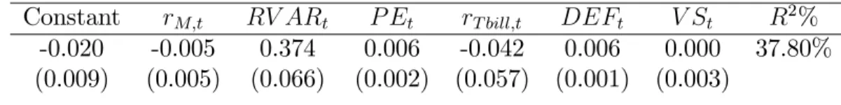
In order for the regression model that generates EV ARt to be consistent with a reasonable data-generating process for market variance, we deviate from standard OLS in two ways. First, we constrain the regression coe¢ cients to produce …tted values (i.e. expected market return variance) that are positive. Second, given that we explicitly consider heteroskedas-ticity of the innovations to our variables, we estimate this regression using Weighted Least Squares (WLS), where the weight of each observation pair (RV ARt+1, xt) is initially based on the previous period’s realized variance, RV ARt1. However, to ensure that the ratio of weights across observations is not extreme, we shrink these initial weights towards equal weights. In particular, we set our shrinkage factor large enough so that the ratio of the largest observation weight to the smallest observation weight is always less than or equal to …ve. Though admittedly somewhat ad hoc, this bound is consistent with reasonable priors on the degree of variation over time in the expected variance of market returns. More impor-tantly, we show in the online appendix that our results are robust to variation in this bound. Both the constraint on the regression’s …tted values and the constraint on WLS observation weights bind in the sample we study.
The …rst-stage regression generating the state variable EV ARt is reported in Table 1, Panel A. Perhaps not surprisingly, past realized variance strongly predicts future realized variance. More importantly, the regression documents that an increase in eitherP EorDEF predicts higher future realized volatility. Both of these results are strongly statistically signif-icant and are a novel …nding of the paper. The predictive power of very persistent variables like P E and DEF indicates a potentially important role for lower-frequency movements in stochastic volatility.
We argue that these empirical patterns are sensible. Investors in risky bonds incorporate their expectation of future volatility when they set credit spreads, as risky bonds are short
the option to default. Therefore we expect higher DEF to predict higher RV AR. The positive predictive relationship between P E and RV AR might seem surprising at …rst, but one has to remember that the coe¢ cient indicates the e¤ect of a change in P E holding constant the other variables, in particular the default spreadDEF. Since the default spread should also generally depend on the equity premium and since most of the variation in P E is due to variation in the equity premium, we can regard P E as purging DEF of its equity premium component to reveal more clearly its forecast of future volatility. We discuss this interpretation further in section 4.4 below.
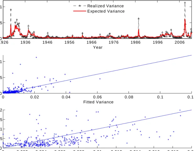
The R2 of the variance forecasting regression is nearly 38%. We illustrate this …t in several ways in Figure 1. The top panel of the …gure shows the movements of RV ARt and EV ARt over time (both variables plotted at time t), illustrating their common low-frequency variation. This panel also highlights occasional spikes in realized varianceRV AR, which generate high subsequent forecasts but are not themselves predicted byEV AR. The middle panel of the …gure plots the realized values at each time t, RV ARt, against the forecast obtained using time t 1information, EV ARt 1, over the whole range of the data. The bottom panel shows the observations for which bothRV ARtandEV ARt 1are less than 0.02 (the bottom left corner of the middle panel). These panels clearly show predictable variation in variance that is captured by our model, and also show the tradeo¤ between frequent small overpredictions of variance and infrequent large underpredictions, caused by the skewness of realized variance.
4.3
Estimation of the VAR and the news terms
4.3.1 VAR estimatesWe estimate a …rst-order VAR as in equation (6), where xt+1 is a 6 1 vector of state variables ordered as follows:
xt+1 = [rM;t+1 EV ARt+1 P Et+1 RT bill;t+1 DEFt+1 V St+1] (19)
so that the real market returnrM;t+1is the …rst element andEV ARis the second element. x is a6 1vector of the means of the variables, and is a6 6matrix of constant parameters. Finally, tut+1is a6 1vector of innovations, with the conditional variance-covariance matrix of ut+1 a constant , so that the parameter 2t scales the entire variance-covariance matrix of the vector of innovations.
The …rst-stage regression forecasting realized market return variance described in the previous section generates the variable EV AR. The theory in Section 3 assumes that 2
t, proxied for byEV AR, scales the variance-covariance matrix of state variable shocks. Thus, as in the …rst stage, we estimate the second-stage VAR using WLS, where the weight of each observation pair (xt+1,xt) is initially based on (EV ARt) 1. We continue to constrain both the weights across observations and the …tted values of the regression forecasting EV AR.
Table 1, Panel B presents the results of the VAR estimation for the full sample (1926:2 to 2011:4).11 We report bootstrap standard errors for the parameter estimates of the VAR that take into account the uncertainty generated by forecasting variance in the …rst stage. Consistent with previous research, we …nd thatP Enegatively predicts future returns, though 11In our robustness test, we show that our …ndings continue to hold if we either estimate our model’s news terms out-of-sample or allow the coe¢ cients in the …rst two regressions of the VAR to vary across the early and modern subsamples.
thet-statistic indicates only marginal signi…cance. The value spread has a negative but not statistically signi…cant e¤ect on future returns. In our speci…cation, a higher conditional variance,EV AR, is associated with higher future returns, though the e¤ect is not statistically signi…cant. Of course, the relatively high degree of correlation among P E, DEF, V S, and EV ARcomplicates the interpretation of the individual e¤ects of those variables. As for the other novel aspects of the transition matrix, both high P E and high DEF predict higher future conditional variance of returns. High past market returns forecast lower EV AR, higher P E, and lower DEF.12
Table 1, Panel C reports the sample correlation matrices of both the unscaled residuals tut+1 and the scaled residualsut+1. The correlation matrices report standard deviations on the diagonals. A comparison of the standard deviations of the unscaled and scaled market return residuals provides a rough indication of the e¤ectiveness of our empirical solution to the heteroskedasticity of the VAR. The scaled return residuals should have unit standard deviation, and our implementation results in a sample standard deviation of 1.14.13
Table 1, Panel D reports the coe¢ cients of a regression of the squared unscaled residuals tut+1 of each VAR equation on a constant andEV AR. These results are broadly consistent with our assumption thatEV ARcaptures the conditional volatility of the market return and other state variables. The coe¢ cient on EV AR in the regression forecasting the squared market return residuals is 1.85, rather than the theoretically expected value of one, but this coe¢ cient is sensitive to the weighting scheme used in the regression. We can reject the null 12One worry is that many of the elements of the transition matrix are estimated imprecisely. Though these estimates may be zero, their non-zero but statistically insigni…cant in-sample point estimates, in conjunction with the highly-nonlinear function that generates discount-rate and volatility news, may result in misleading estimates of risk prices. However, the online appendix shows that we continue to …nd an economically signi…cant negative volatility beta for value-minus-growth bets if we instead employ a partial VAR where, via a standard iterative process, only variables with t-statistics greater than 1.0 are included in each VAR regression.
13A comparison of the unscaled and scaled autocorrelation matrices, in the online appendix, reveals in ad-dition that much of the sample autocorrelation in the unscaled residuals is eliminated by our WLS approach.
hypothesis that all six regression coe¢ cients are jointly zero or negative. This evidence is consistent with the volatilities of all innovations being driven by a common factor, as we assume, although of course it is possible that empirically, other factors also in‡uence the volatilities of certain variables.
4.3.2 News terms
The top panel of Table 2 presents the variance-covariance matrix and the standard devia-tion/correlation matrix of the news terms, estimated as described above. Consistent with previous research, we …nd that discount-rate news is nearly twice as volatile as cash-‡ow news.
The interesting new results in this table concern the variance news term NV. First, news about future variance has signi…cant volatility, with nearly a third of the variability of discount-rate news. Second, variance news is negatively correlated ( 0:12) with cash-‡ow news. As one might expect from the literature on the “leverage e¤ect” (Black, 1976; Christie, 1982), news about low cash ‡ows is associated with news about higher future volatility. Third, NV is close to uncorrelated ( 0:03) with discount-rate news.14 The net e¤ect of these correlations, documented in the lower left panel of Table 2, is a correlation close to zero (again 0:03) between our measure of volatility news and contemporaneous market returns.
The lower right panel of Table 2 reports the decomposition of the vector of innovations 2
tut+1 into the three terms NCF;t+1; NDR;t+1, and NV;t+1. As shocks to EV AR are just a linear combination of shocks to the underlying state variables, which includes RV AR, we 14Though the point estimate of this correlation is negative, the large standard error implies that we cannot reject the “volatility feedback e¤ect” (Campbell and Hentschel, 1992; Calvet and Fisher, 2007), which generates a positive correlation. For related research see French, Schwert, and Stambaugh (1987).
“unpack”EV AR to express the news terms as a function ofrM,P E,RT bill,V S,DEF, and RV AR. The panel shows that innovations to RV AR are mapped more than one-to-one to news about future volatility. However, several of the other state variables also drive news about volatility. Speci…cally, we …nd that innovations in P E,DEF, and V S are associated with news of higher future volatility. This panel also indicates that all state variables with the exception of RT bill are statistically signi…cant in terms of their contribution to at least one of the three news terms. We choose to leave RT bill in the VAR, though its presence in the system makes little di¤erence to our conclusions.
Figure 2 plots theNCF, NDR andNV series. To emphasize lower-frequency movements and to improve the readability of the …gure, we …rst normalize each series by its standard deviation and then smooth (for plotting purposes only) using an exponentially-weighted moving average with a quarterly decay parameter of 0:08. This decay parameter implies a half-life of approximately two years. The pattern of NCF and NDR we …nd is consistent with previous research, for example, Figure 1 of CV (2004). As a consequence, we focus on the smoothed series for market variance news. There is considerable time variation in NV, and in particular we …nd episodes of news of high future volatility during the Great Depression and just before the beginning of World War II, followed by a period of little news until the late 1960s. From then on, periods of positive volatility news alternate with periods of negative volatility news in cycles of three to …ve years. Spikes in news about future volatility are found in the early 1970s (following the oil shocks), in the late 1970s and again following the 1987 crash of the stock market. The late 1990s are characterized by strongly negative news about future returns, and at the same time higher expected future volatility. The recession of the late 2000s is instead characterized by strongly negative cash-‡ow news, together with a spike in volatility of the highest magnitude in our sample. The recovery from the …nancial crisis has brought positive cash-‡ow news together with news about lower future volatility.
4.4
Predicting long-run volatility
The predictability of volatility, and especially of its long-run component, is central to this paper. In the previous sections, we have shown that volatility is strongly predictable, specif-ically by variables beyond lagged realizations of volatility itself: P E and DEF contain essential information about future volatility. We have also proposed a VAR-based method-ology to construct long-horizon forecasts of volatility that incorporate all the information in lagged volatility as well as in the additional predictors likeP E and DEF.
We now ask how well our proposed long-run volatility forecast captures the long-horizon component of volatility. In the online appendix, we regress realized, discounted, annualized long-run variance up to periodh,
LHRV ARh = 4 h j=1 j 1RV ARt+j h j=1 j 1 ; (20)
on the variables included in our VAR system, the VAR long-horizon forecast, and some alternative forecasts of long-run variance. We focus on a 10-year horizon (h= 40) as longer horizons come at the cost of fewer independent observations; however, the online appendix con…rms that our results are robust to horizons ranging from one to 15 years.
As alternatives to the VAR approach, we estimate two standard GARCH-type models, speci…cally designed to capture the long-run component of volatility: the two-component exponential (EGARCH) model proposed by Adrian and Rosenberg (2008), and the frac-tionally integrated (FIGARCH) model of Baillie, Bollerslev, and Mikkelsen (1996). We …rst estimate both GARCH models using the full sample of daily returns and then generate the appropriate forecast of LHRV AR40. To these two models, we add the set of variables from our VAR, and compare the forecasting ability of these di¤erent models. We …nd that while the EGARCH and FIGARCH forecasts do forecast long-run volatility, our VAR variables
provide as good or better explanatory power, and RV AR, P E and DEF are strongly sta-tistically signi…cant. Our long-run VAR forecast has a coe¢ cient of 1.02, which remains highly signi…cant at 0.82 even in the presence of the FIGARCH forecast. We also …nd that DEF does not predict long-horizon volatility in the presence of our VAR forecast, implying that the VAR model captures the long-horizon information in the default spread.
The online appendix also examines more carefully the links between P E, DEF, and LHRV AR40. We …nd that by itself, P E has almost no information about low-frequency variation in volatility. In contrast,DEF forecasts nearly 22% of the variation inLHRV AR40. Furthermore, if we use the component of DEF that is orthogonal to P E, which we call DEF O or theP E-adjusted default spread, theR2 increases to over 51%. Our interpretation of these results is thatDEF contains information about future volatility because risky bonds are short the option to default. However, DEF also contains information about future aggregate risk premia. We know from previous work that much of the variation inP Ere‡ects aggregate risk premia. Therefore, includingP E in the volatility forecasting regression cleans up variation in DEF resulting from variation in aggregate risk premia and thus sharpens the link between DEF and future volatility. Since P E and DEF are negatively correlated (default spreads are relatively low when the market trades rich), bothP E andDEF receive positive coe¢ cients in the multiple regression.
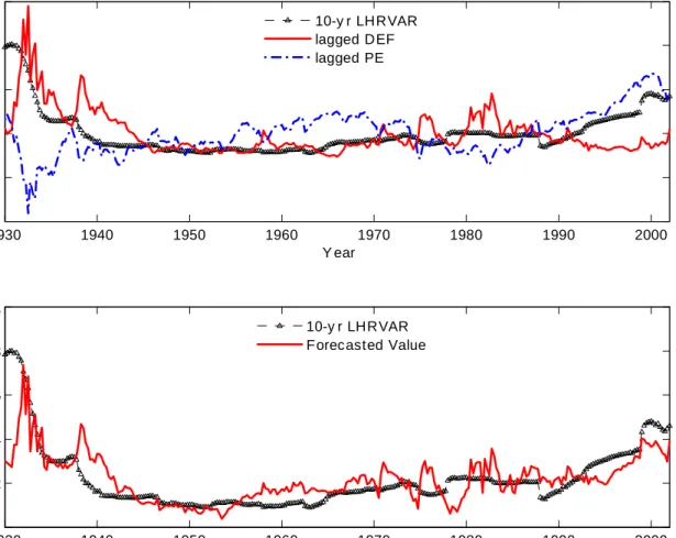
Figure 3 provides a visual summary of the long-run volatility-forecasting power of our key VAR state variables and our interpretation. The top panel plots LHRV AR40 together with lagged DEF and P E. The graph con…rms the strong negative correlation between P E and DEF (correlation of -0.6) and highlights the way both variables track long-run movements in long-run volatility. To isolate the contribution of the default spread in pre-dicting long run volatility, the bottom panel plots LHRV AR40 together with DEF O, the P E-adjusted default spread that is orthogonal to the market’s smoothed price-earnings ratio.
The contrasting behavior of DEF and DEF O in the two panels during episodes such as the tech boom help illustrate the workings of our story. Taken in isolation, the relatively stable default spread throughout most of the late 1990s would predict little change in future market volatility. However, once the declining equity premium over that period is taken into account (as shown by the rapid increase in P E), one recognizes that a high P E-adjusted default spread in the late 1990s actually forecasted much higher volatility ahead.
As a further check on the usefulness of our VAR approach, in the online appendix we compare our variance forecasts to option-implied variance forecasts over the period 1998– 2011. We …nd that when both the VAR and option data are used to predict realized variance, the VAR forecasts drive out the option-implied forecasts while remaining statistically and economically signi…cant.
Taken together, these results make a strong case that credit spreads and valuation ratios contain information about future volatility not captured by simple univariate models, even those designed to …t long-run movements in volatility. Furthermore, our VAR method for calculating long-horizon forecasts preserves this information.
5
Estimating the ICAPM Using Equity Portfolios Sorted
by Size, Value, and Risk
5.1
Construction of test assets
In addition to the VAR state variables, our analysis requires excess returns on a set of test assets. In this section, we construct several sets of equity portfolios sorted by value, size, and risk estimates from our model. Full details on the construction method are provided in
the online appendix.
Since the long-term investor in our model is assumed to hold the equity market, we measure all excess returns relative to the market portfolio. Our primary cross section consists of the excess returns over the market on 25 portfolios sorted by size and value (ME and BE/ME), studied in Fama and French (1993), extended in Davis, Fama, and French (2000), and made available by Professor Kenneth French on his website. To this cross-section, we add the excess return on a Treasury bill over the market (the negative of the usual excess return on the market over a Treasury bill), which gives us an initial set of 26 characteristic-sorted test assets.
We incorporate additional assets in our tests in order to guard against the concerns of Daniel and Titman (1997, 2012) and Lewellen, Nagel, and Shanken (2010) that characteristic-sorted portfolios may have a low-order factor structure that is easily …t by spurious models. In particular, we construct a second set of six risk-sorted portfolios, double-sorted on past multiple betas with market returns and variance innovations (approximated by a weighted average of changes in the VAR explanatory variables).
We also consider excess returns on equity portfolios that are formed based on both characteristics and past exposures to variance innovations. One possible explanation for our …nding that growth stocks hedge volatility relative to value stocks is that growth …rms are more likely to hold real options, whose value increases with volatility. To test this interpretation, we …rst sort stocks based on two …rm characteristics that are often used to proxy for the presence of real options and that are available for a large percentage of …rms throughout our sample period: BE/ME and idiosyncratic volatility (ivol). Having formed nine portfolios using a two-way characteristic sort, we split each of these portfolios into two subsets based on pre-formation estimates of each stock’s simple beta with variance innovations. One might expect that sorts on simple rather than partial betas will be
more e¤ective in establishing a link between pre-formation and post-formation estimates of volatility beta, since the market is correlated with volatility news. This gives us 18 portfolios sorted on both characteristics and risk.
Combining all the above portfolios, we have a set of 50 test assets. We …nally create managed or scaled versions of all these portfolios by interacting them with our volatility forecast EV AR. The managed portfolios increase their exposure to test assets at times when market variance is expected to be high. With both unscaled and scaled portfolios, we have a total of 100 test assets.15
Previous research, particularly CV (2004), has documented important di¤erences in the risks of value stocks in the periods before and after 1963. Accordingly we consider two main subsamples, which we call early (1931:3-1963:3) and modern (1963:4-2011:4). A successful model should be able to …t the cross-section of test asset returns in both these periods with stable parameters.
5.2
Beta measurement
We …rst examine the betas implied by the covariance form of the model in equation (16). We cosmetically multiply and divide all three covariances by the sample variance of the unex-pected log real return on the market portfolio to facilitate comparison to previous research,
de…ning i;CFM Cov(ri;t; NCF;t) V ar(rM;t Et 1rM;t) , (21) i;DRM Cov(ri;t; NDR;t) V ar(rM;t Et 1rM;t) , (22)
and i;VM Cov(ri;t; NV;t) V ar(rM;t Et 1rM;t)
. (23)
The risk prices on these betas are just the variance of the market return innovation times the risk prices in equation (16).
We estimate cash-‡ow, discount-rate, and variance betas using the …tted values of the market’s cash ‡ow, discount-rate, and variance news estimated in the previous section. Speci…cally, we estimate simple WLS regressions of each portfolio’s log returns on each news term, weighting each time-t+ 1 observation pair by the weights used to estimate the VAR in Table 1 Panel B. We then scale the regression loadings by the ratio of the sample variance of the news term in question to the sample variance of the unexpected log real return on the market portfolio to generate estimates for our three-beta model.
5.2.1 Characteristic-sorted portfolios
Table 3 Panel A shows the estimated betas for the characteristic-sorted portfolios over the 1931-1963 period. To save space, we omit the betas for portfolios in the second and fourth quintiles of each characteristic, retaining only the …rst, third, and …fth quintiles. The full table can be found in the online appendix.
The portfolios are organized in a square matrix with growth stocks at the left, value stocks at the right, small stocks at the top, and large stocks at the bottom. At the right edge of the matrix we report the di¤erences between the extreme growth and extreme value
portfolios in each size group; along the bottom of the matrix we report the di¤erences between the extreme small and extreme large portfolios in each BE/ME category. The top matrix displays post-formation cash-‡ow betas, the middle matrix displays post-formation discount-rate betas, while the bottom matrix displays post-formation variance betas. In square brackets after each beta estimate we report a standard error, calculated conditional on the realizations of the news series from the aggregate VAR model.
In the pre-1963 sample period, value stocks (except those in the smallest size quintile) have both higher cash-‡ow and higher discount-rate betas than growth stocks. An equal-weighted average of the extreme value stocks across all size quintiles has a cash-‡ow beta 0.12 higher than an equal-weighted average of the extreme growth stocks. The average di¤erence in estimated discount-rate betas, 0.25, is in the same direction. Similar to value stocks, small stocks have consistently higher cash-‡ow betas and discount-rate betas than large stocks in this sample (by 0.16 and 0.36, respectively, for an equal-weighted average of the smallest stocks across all value quintiles relative to an equal-weighted average of the largest stocks). These di¤erences are extremely similar to those in CV (2004), despite the exclusion of the 1929-1931 subperiod, the replacement of the excess log market return with the log real return, and the use of a richer, heteroskedastic VAR.
The new …nding in the top portion of Table 3 Panel A is that value stocks and small stocks are also riskier in terms of volatility betas. An equal-weighted average of the extreme value stocks across all size quintiles has a volatility beta 0.06 lower than an equal-weighted average of the extreme growth stocks. Similarly, an equal-weighted average of the smallest stocks across all value quintiles has a volatility beta that is 0.06 lower than an equal-weighted average of the largest stocks. In summary, value and small stocks were unambiguously riskier than growth and large stocks over the 1931-1963 period.
doc-umented in this subsample by CV (2004), value stocks still have slightly higher cash-‡ow betas than growth stocks, but much lower discount-rate betas. Our new …nding here is that value stocks continue to have much lower volatility betas, and the spread in volatility betas is even greater than in the early period. The volatility beta for the equal-weighted average of the extreme value stocks across size quintiles is 0.11 lower than the volatility beta of an equal-weighted average of the extreme growth stocks, a di¤erence that is more than 85% higher than the corresponding di¤erence in the early period.
These results imply that in the post-1963 period where the CAPM has di¢ culty explain-ing the low returns on growth stocks relative to value stocks, growth stocks are relative hedges for two key aspects of the investment opportunity set. Consistent with CV (2004), growth stocks hedge news about future real stock returns. The novel …nding of this paper is that growth stocks also hedge news about the variance of the market return.
One interesting aspect of these …ndings is the fact that the average V of the 25 size-and book-to-market portfolios changes sign from the early to the modern subperiod. Over the 1931-1963 period, the average V is -0.10 while over the 1964-2011 period this average becomes 0.06. Of course, given the strong positive link between P E and volatility news documented in the lower right panel of Table 2, one should not be surprised that the market’s V can be positive. Nevertheless, in the online appendix we study this change in sign more carefully. We show that the market’s beta with realized volatility has remained negative in the modern period, highlighting the important distinction between realized and expected future volatility. We also show that the change in the sign of V is driven by a change in the correlation between the aggregate market return and the change in DEF O, our simple proxy for news about long-horizon variance.
5.2.2 Risk-sorted portfolios
Panels C and D of Table 3 show the estimated betas for the six risk-sorted portfolios over the 1931-1963 and post-1963 periods. The portfolios are organized in a rectangular matrix with low market-beta stocks at the left, high market-beta stocks at the right, low volatility-beta stocks at the top, and high volatility-beta stocks at the bottom. Otherwise the format is the same as that of Panels A and B.
In the pre-1963 sample period, high market-beta stocks have both higher cash-‡ow and higher discount-rate betas than low market-beta stocks. Similarly, low volatility-beta stocks have higher cash-‡ow betas and discount-rate betas than high volatility-beta stocks. High market-beta stocks also have lower volatility betas, but sorting stocks by their past volatility betas induces little spread in post-formation volatility betas. Putting these results together, in the 1931-1963 period high market-beta stocks and low volatility-beta stocks were unam-biguously riskier than low market-beta and high volatility-beta stocks.
In the post-1963 (modern) period, high market-beta stocks again have higher cash-‡ow and higher discount-rate betas than low market-beta stocks. However, high market-beta stocks now have higher volatility betas and are therefore safer in this dimension. This pattern may not be surprising given our …nding that the aggregate market portfolio itself has a positive volatility beta in the modern period. The important implication is that our three-beta model with priced volatility risk helps to explain the well-known result that stocks with high past market betas have o¤ered relatively little extra return in the past 50 years (Fama and French, 1992; Frazzini and Pedersen, 2013).
In the modern period, sorts on volatility beta generate an economically and statistically signi…cant spread in post-formation volatility beta. These high volatility-beta portfolios also tend to have higher discount-rate betas and lower cash-‡ow betas, though the patterns are
not uniform.
We also examine test assets that are formed based on both characteristics and risk es-timates. The online appendix reports the estimated betas for the 18 BE/ME-ivol-b V AR -sorted portfolios in both the early and modern sample periods. In the early period, …rms with higherivolhave lower post-formation volatility betas regardless of their book-to-market ratio. Consistent with this …nding, higher ivol stocks have higher average returns. In the modern period, however, we …nd that among stocks with low BE/ME, …rms with higherivol have higher post-formation volatility betas and lower average returns; but these patterns reverse among stocks with high BE/ME.
We argue that these di¤erences make economic sense. High idiosyncratic volatility in-creases the value of growth options, which is an important e¤ect for growing …rms with ‡exible real investment opportunities, but much less so for stable, mature …rms. Valuable growth options in turn imply high betas with aggregate volatility shocks. Hence high idio-syncratic volatility naturally raises the volatility beta for growth stocks more than for value stocks. This e¤ect is stronger in the modern sample where growing …rms with ‡exible investment opportunities are more prevalent.
Taken together, the …ndings from the characteristic- and risk-sorted test assets suggest that volatility betas vary with multiple stock characteristics, and that techniques that take this into account may be more e¤ective in generating a spread in post-formation volatility beta.
5.3
Model estimation
we report our results in terms of the expected return-beta representation from equation (16), rescaled by the variance of market return innovations as in section 5.2:
Ri Rj =g1bi;CFM +g2bi;DRM +g3bi;VM +ei; (24)
where bars denote time-series means and betas are measured using returns relative to the reference asset. Recall that we use the aggregate equity market as our reference asset but include the T-bill return as a test asset, so that our model not only prices cross-sectional variation in average returns, but also prices the average di¤erence between stocks and bills. We evaluate the performance of …ve asset pricing models, all estimated via GMM: 1) the traditional CAPM that restricts cash-‡ow and discount-rate betas to have the same price of risk and sets the price of variance risk to zero; 2) the two-beta intertemporal asset pricing model of CV (2004) that restricts the price of discount-rate risk to equal the variance of the market return and again sets the price of variance risk to zero; 3) our three-beta intertemporal asset pricing model that restricts the price of discount-rate risk to equal the variance of the market return and constrains the prices of cash-‡ow and variance risk to be related by equation (10), with = 0:95 per year; 4) a partially-constrained three-beta model that restricts the price of discount-rate risk to equal the variance of the market return but freely estimates the other two risk prices (e¤ectively decoupling and !); and 5) an unrestricted three-beta model that allows free risk prices for cash-‡ow, discount-rate, and volatility betas.
5.3.1 Model estimates
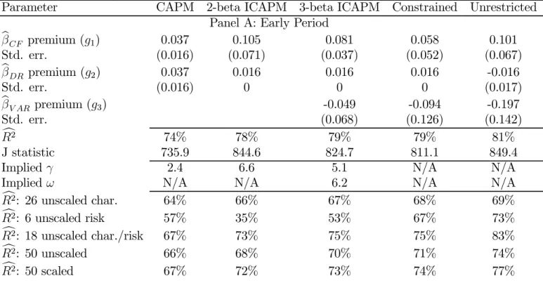
Table 4 reports the results of pricing tests for both the early sample period 1931-1963 (Panel A) and the modern sample period 1963-2011 (Panel B). In each case we price the complete
set of test assets described in section 5.1; the online appendix reports the results of tests that price the 25 size- and book-to-market-sorted portfolios in isolation. The table has …ve columns, one for each of our asset pricing models. The …rst six rows of each panel in Table 4 are divided into three sets of two rows. The …rst set of two rows corresponds to the premium on cash-‡ow beta, the second set to the premium on discount-rate beta, and the third set to the premium on volatility beta. Within each set, the …rst row reports the point estimate in fractions per quarter, and the second row reports the corresponding standard error. Below the premia estimates, we report the R2 statistic for a cross-sectional regression of average market-adjusted returns on our test assets onto the …tted values from the model as well as the J statistic. In the next two rows of each panel, we report the implied risk-aversion coe¢ cient, , which can be recovered as g1=g2, as well as the sensitivity of news about risk to news about market variance, !, which can be recovered as 2g3=g2. The …ve …nal rows in each panel report the cross-sectional R2 statistics for various subsets of the test assets.
Table 4 Panel A shows that in the early subperiod, all models do a relatively good job pricing these 100 test assets. The cross-sectional R2 statistic is 74% for the CAPM, 78% for the two-beta ICAPM, and 79% for our three-beta ICAPM. Consistent with the claim that the three-beta model does a good job describing the cross section, the constrained and the unrestricted factor model barely improve pricing relative to the three-beta ICAPM in Panel A. Despite this apparent success, all models are rejected based on the standardJ test. This may not be surprising, given that even the empirical three-factor model of Fama and French (1993) is rejected by this test when faced with the 25 size- and book-to-market-sorted portfolios.
In stark contrast, Panel B documents that in the modern subperiod, the CAPM fails to price not only the characteristic-sorted test assets already considered in previous work, but also risk-sorted and variance-scaled portfolios. The cross-sectional R2 of the CAPM is