Universidade de São Paulo
2015-07
An evolutionary sampling approach for
classification with imbalanced data
International Joint Conference on Neural Network, 2015, Killarney.
http://www.producao.usp.br/handle/BDPI/49272
Downloaded from: Biblioteca Digital da Produção Intelectual - BDPI, Universidade de São Paulo
Biblioteca Digital da Produção Intelectual - BDPI
An Evolutionary Sampling Approach for
Classification with Imbalanced Data
Everlandio R. Q. Fernandes U niversidade de Sao Paulo Instituto de Ciencias Matematicas
e de Computa<;ao (ICMC) Sao Carlos, Sao Paulo Email: [email protected]
Andre c.P.L.F. de Carvalho Universidade de Sao Paulo Instituto de Ciencias Matematicas
e de Computa<;ao (ICMC) Sao Carlos, Sao Paulo Email: [email protected]
Andre L. V. Coelho Universidade de Fortaleza Programa de Pos-Gradua<;ao em
Informatica Aplicada (PPOIA) Fortaleza, Ceara Email: [email protected]
Abstract-In some practical classification problems in which the number of instances of a particular class is much lower/higher than the instances of the other classes, one commonly adopted strategy is to train the classifier over a small, balanced portion of the training data set. Although straightforward, this procedure may discard instances that could be important for the better discrimination of the classes, affecting the performance of the resulting classifier. To address this problem more properly, in this paper we present MOGASamp (after Multiobjective Genetic Sampling) as an adaptive approach that evolves a set of samples of the training data set to induce classifiers with optimized predictive performance. More specifically, MOGASamp evolves balanced portions of the data set as individuals of a multi objective genetic algorithm aiming at achieving a set of induced classifiers with high levels of diversity and accuracy. Through experiments involving eight binary classification problems with varying levels of class imbalancement, the performance of MOGASamp is compared against the performance of six traditional methods. The overall results show that the proposed method have achieved a noticeable performance in terms of accuracy measures.
I. INTRODUCTION
Several classification problems present data with imbal anced class distributions. Such an imbalancement occurs nat urally in some practical applications, such as in financial data [1], where the number of instances in the "default" class (minority class) is generally lower than the number of instances in the "non-default" class (majority class). Imbalanced data sets may affect the predictive performance of some classical classification algorithms because these algorithms assume that the data has a balanced distribution of classes and that the same cost of misclassification applies to all classes [2].
A commonly strategy used for classification with imbal anced data sets is to select a balanced set of instances from each class. This means that the number of instances of the minority class will be equal to the number of instances of the majority class. This strategy is used to generate a classification model that is not detrimental to the minority class. However, this procedure may not be effective in some cases, since the final classification model may not take into account relevant instances for better discrimination between the classes, leading to a decrease in the predictive accuracy of the classifier.
In order to overcome this problem, ensembles of classifiers have been considered. Ensembles are designed to increase the accuracy of a single classifier by inducing separately a set of
978-1-4799-1959-8/15/$31.00 @2015 IEEE
hypotheses and combining their decisions by some consensus operator [3]. The generalization ability of an ensemble is usually higher than that of a single classifier. In [4] the authors present a formal demonstration of this. Although ensembles tend to perform better than their members, their construction is not an easy task. According to [5], an ensemble of classifiers with high accuracy implies two conditions: each base classifier has an accuracy higher than 50%; and they should be different from each other. Two classifiers are considered different from each other if their misclassifications are made in different instances of the same test set i.e., they should disagree as much as possible in their outcomes [6].
Therefore, diversity and accuracy are the two main criteria that should be taken into account to generate an effective ensemble of classifiers. In this context, some metrics have been proposed to measure the diversity of the classifiers, such as the Pairwise Failure Crediting (PFC) [7] and the negative correlation in the Negative Correlation Learning (NCL) ap proach [8]. However, there is a trade-off on what should be the optimal measures of diversity and accuracy, since these are two conflicting criteria [9]. To handle this situation, the use of Multiobjective Evolutionary Algorithms (MOEA) seems to be an interesting solution, since MOEA can deal nicely with conflicting objectives in the learning process. Such algorithms evolve simultaneously a set (aka front) of non-dominated solutions over two or more objectives, without requiring the imposition of preferences on the objectives. In the case of ensembles of classifiers, the objectives are the two criteria of accuracy and diversity.
In this context, this paper proposes a new approach, namely MOGASamp (Multiobjective Genetic Sampling), to deal with the problem of imbalanced data sets aiming at an ensemble of classifiers with high predictive performance. The goal of MOGASamp is to construct an ensemble of classifiers induced from balanced samples of the training data set. For this, a customized MOEA will evolve combinations of instances in balanced samples, guided by the performance of the classifiers induced by these samples. This strategy allows one to obtain a set of balanced samples from the imbalanced data set that induces classifiers with high accuracy and diversity.
In order to assess the novel approach, experimental tests were performed using several different imbalanced data sets. Comparative evaluations have demonstrated that MOGASamp
can outperform traditional algorithms, such as AdaBoost and Bagging, being a good option for dealing with imbalanced data sets.
The remainder of this paper is structured as follows: Sec tion 2 provides a review of related work. Section 3 discusses the evaluation metrics considered in this work. Section 4 introduces the main ingredients of the MOGASamp technique. Section 5 shows the experimental analysis and Section 6 concludes the paper.
II. LITERATURE REV IEW
Most of the studies found in the literature for classification with imbalanced data sets rely on two approaches [10]. The first approach allocates different costs to classes during the in duction of the classification model [11]. The second approach is based on data resampling (subsampling or oversampling). In subsampling, instances from the majority class are removed, while oversampling the instances of the minority class are replicated or synthetic data are generated.
Although using a simple strategy, the subsampling ap proach when performed randomly may discard important data. To address this problem, a directed subsampling method can be used to detect and eliminate less representative portions of the data. This is the strategy used by the One-Sided Selection (OSS) technique [12], which removes instances from the majority class that are redundant, noisy, and/or close to the boundary between the classes. The border instances are detected by applying Tomek links, and the instances that are distant from the decision boundary (redundant instances) are discovered by Condensed Nearest Neighbor (CNN) [13].
On the other hand, considering the oversampling approach, the replication of instances tends to increase the computational cost of the process [14]. These approaches can be categorized into random or classic oversampling and synthetic oversam piing. The classic oversampling method is a non-heuristic method that add instances through the random replication of the minority class instances. This kind of oversampling sometimes creates very specific rules, leading to overfitting [15]. However, synthetic oversampling methods add instances by generating synthetic minority class instances. The gener ated instances add essential information to the original data set that may help improve the classifiers performance. The interpolation technique is commonly used to generate synthetic data, such as in SMOTE (Synthetic Minority Oversampling Technique) [16]. SMOTE finds the k nearest neighbors of each instance of the minority class and, then, synthetic instances are generated along the line that connects the instance with its k nearest neighbors. Although SMOTE has proved to be an effective tool for handling the class imbalancement, it may overgeneralize the minority class, once it does not consider the distribution of majority class neighbors. As a result, it may increase the overlapping between classes [17].
Other studies use ensembles of classifiers to deal with imbalanced data set, such as Bagging [18] and Boosting [19]. The Bagging approach trains a set of base classifiers with different samples of the training data set. The sampling is performed with replacement and each sample has the same size of the original training data set. After obtaining the base
classifiers, it combines them by majority voting, and the most voted class is predicted for a new instance.
The AdaBoost approach, the most representative algorithm in the Boosting family, uses the whole training data set to create classifiers serially. In each iteration, AdaBoost gives more emphasis to the instances that were incorrectly classified in the previous iteration. For this, the weights of incorrectly classified instances are increased and the weights of correctly classified instances are decreased. Finally, when a new instance is presented, each base classifier gives its vote, weighted by its overall accuracy, and the label of the new instance is selected based on the majority of votes.
III. PERFORM ANCE EVALUATION
This section presents measures to evaluate the performance of the classifiers in imbalanced domains and to evaluate the diversity of an ensemble of classifiers.
A. Accuracy
An effective measure to evaluate the performance of a classifier is the rate of classification errors made in each class [2]. Such measure can be obtained using a confusion matrix. Each column of this matrix represents the instances in a predicted class, while each row represents the instances in an actual class. Elements along the main diagonal represent the correct classifications, number of true negatives (TN) and true positives (TP), while the off-diagonal elements represent the classification errors, number of false positives (FP) and false negatives (FN). From the confusion matrix, it is possible to extract two independent measures: True Positive Rate (Eq. 1) and True Negative Rate (Eq. 2). These two measures evalu ate the performance on the positive (minority) and negative (majority) classes, respectively.
TP = TP r TP+FN TN = TN r TN + FP (1) (2)
However, the goal is to achieve a good prediction in both classes (minority and majority) when dealing with a binary classification problem. So, it is necessary to combine these individual measures (T Pr and T Nr), since they are not useful when used alone. These measures are combined by the Receiver Operating Characteristic (ROC) curve [20], which shows the relationship between the benefits and the classification costs in relation to the distribution of the data. So, we say that a classification model is better than another if its ROC curve dominates the other. When it is necessary to encode the ROC curve into a single scalar value, the most common strategy is to calculate the Area under the ROC Curve (AUC) [21].
B. Diversity
If we have a perfect classifier that makes no errors, then we do not need an ensemble. If, however, the classifier does make some errors, then we can try to complement it with another classifier, which makes errors on different objects. Therefore,
Database YeastMEl YeastMit YeastME3 Spect Ion German Haberman CMC
Imbalance Ratio 1:33 1:5 1:8 1:4 1:2 1:2 1:3 1:3
Total of Instances 1484 1484 1484 267 351 1000 306 1473
TABLE I: Databases Used for the Experimental Tests
as mentioned earlier, the success of an ensemble depends on the diversity of the prediction errors generated by their base classifiers.
The diversity of an ensemble can be measured in two dif ferent ways: 1) considering the diversity of a pair of classifiers and then the average is obtained for all pairs diversity (Pairwise Measures); or 2) considering all the classifiers together and calculating a unique diversity value of the ensemble (Non pairwise Measures) [22].
The Pairwise Failure Crediting (PFC) measure [7] calcu lates the distance between the failure patterns taking each pair of individuals. A failure pattern is a string of Os and Is indicating success or failure of the classifier. The accu mulated differences on each individuals in the ensemble is used to compute the diversity of the individual members with respect to the ensemble, i.e. how different a member is with respect to others in the ensemble. The PFC measure has been employed in MOGASamp to achieve a set of samples that induce classifiers with good performance when dealing with imbalanced data sets.
IV. MOGASAMP
The goal of the proposed method is to generate a set of samples to induce base classifiers that will compose an ensemble of classifiers, so that that these classifiers have high accuracy with the most diversity as possible. For this purpose, MOGASamp adopts a multiobjective genetic algorithm to evolve a selection of samples and to evaluate the classifiers induced by these samples based on accuracy and diversity.
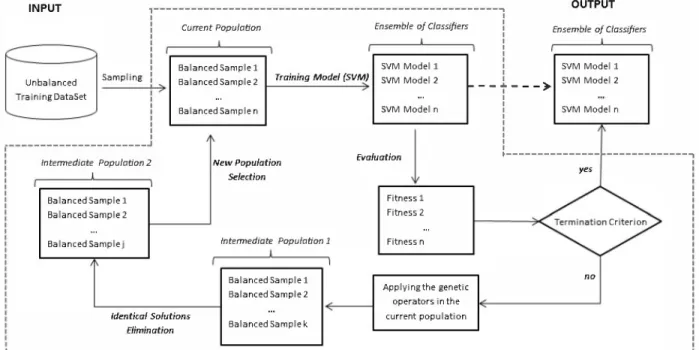
Figure 1 outlines the proposed method. In the following subsections, we will detail each of its main steps.
A. Sampling and the Training Models
In the first step we obtain n balanced samples from the
training data set. This means that each sample will have an equal amount of instances of each class. The size of the samples is chosen based on the number of instances of the minority class. However, we use only 90% of the instances of the minority class to compose the samples. The remain 10% of the instances are used to perform the validation in the evolution process (refer to the next step). These samples are obtained without replacement. Each sample represents an individual of the population of the Genetic Algorithm (GA). These samples are encoded by a vector with dimensionality equal to the sample size. The cells of this vector represent the training instances that are part of the sample, and for each individual an SVM model is generated.
B. Evaluation
The obtained SVM model of each individual is validated using the instances that were not used to obtain the samples,
i.e. the remaining 10% of the instances of the minority class and the other instances of the majority class. The AUC metric is calculated based on the performance of this model over the validation data. The PFC is also calculated for each individual using a pair-wise comparison with all individuals of the current population.
In this MOGASamp, the fitness of each individual is given by the AUC and PFe. These two metrics are used to compose a dominance rank [23] of the solutions. The dominance rank of a given solution is the number of other solutions in the population that dominate it. A solution Xl is said to dominate
another solution X2 if Xl is no worse than X2 in all objectives
and Xl is strictly better than X2 in at least one objective
[24]. A nondominated solution will have the best fitness of 0, while high fitness values indicate poor-performing solutions, i.e., solutions dominated by many individuals.
C. Genetic Operators
The dominance rank is used to select the individuals that will breed a new generation using the genetic operators (reproduction and mutation). This selection is performed using a tournament of size 3. If a tie occurs, we consider that the winner will be the one with highest AUe. The quantity of parents selected will be equal to the quantity of individuals of the current population. For each selected pair of parents, two new individuals are generated by merging the instances from the minority class of a parent with the instances from the majority class of another parent, and vice-versa. The mutation occurs in a percentage of the offspring generated. The instances of a random portion of the sample that represents an individual is changed by a new sampling, maintaining the proportion of classes.
D. Elimination of Identical Solutions
After applying the genetic operators, identical individuals can occur, especially when the imbalance ratio is not high (less than 1:6). This fact was observed in our experimental tests. Identical individuals with high fitness have a higher probability of being selected for reproduction and for future generations, increasing even further the number of replicated solutions. However, the goal of this work is to have a diverse ensemble of classifiers with a high accuracy. For this reason, after reproduction, identical individuals are eliminated. Afterwards, if the number of individuals is less than the initial population size, a new reproduction and mutation process is performed.
E. New Generation and Stop Criterion
The selection of the individuals that will compose the new generation is based on the non-dominance of each individual. First, individuals with higher levels of non-dominance are selected, then only those who are not dominated by the first, and so on, until the default population size is reached. This
OUTPUT
INPUT ,---�
Curren t Population Ensemble of Classifiers : Ensemble of Classifiers I --Balanced Sample 1 I 1 : I SVM Modell I I SVM Modell Un Trai
balanced Sampling Balanced Sample 2
I
Training Model (SVM) SVM Model 2 I SVM Model 2
) --t---» n i ng DataSet ... ... I .. ; . SVM Model n I SVM Model n --- Balanced Sample n I I I
1
I I I' --- I I f.,aJuation t------Intermediate Population 2 New Population
yes I Selection I I ---. BalancedSamplel Fitness 1 BaiancedSample2 Fitness 2
Termination Criterion ...
...
BalancedSamplei Intermediate Population 1 Fitness n
I I I
no Balanced Sample 1
Balanced Sample 2 Applying the genetiC
operators in the
Identical Solutions ... � current population
Elimination Balanced Sample k ,
,---Fig. 1: MOGASamp - Multiobjective Genetic Sampling
process repeats until the fixed number of generations and/or the maximum AVC value is reached, i.e. AVC = 1.0.
The classification models of all individuals in the final population compose the ensemble of classifiers. When a new instance is presented to the classifiers, its class is determined by majority voting considering the output of all classifiers.
V. EXPERIMENTAL RESULTS
Eight binary classification data sets with different imbal ance ratio were used in our empirical assessment. These data sets were obtained from the VCI Repository [25] and are summarized in Table I. For each data set, half of the instances of each class were randomly chosen for the training set and the other half as the test set. This ensures that both the training and test sets maintain the same class proportion as in the original data set.
MOGASamp was compared against six well-known re sampling and classification techniques from the literature. The resampling techniques used were: SMOTE; Classical subsam piing (random); Directed subsampling (OSS); and Classical oversampling. The classification techniques used were: Bag ging and AdaBoost. For the resampling algorithms, after the process of rebalancing the classes, the SVM algorithm was used to generate the classification model.
MOGASamp was performed with a population of 40 indi viduals, a maximum of 20 generation and 5% as mutation rate. The SMOTE parameters used were: 200% as the percentage of oversampling and undersampling, 5 as the number of the neighbors. These are the default parameter values specified in the package used [26]. The classic Subsampling and Oversam piing were performed until resulting in a balanced dataset. For the OSS technique, it is not necessary to set any parameter. The package used for OSS, classic Subsampling and Oversampling
was that available in [27]. For Bagging and AdaBoost 100 iterations were used, as well as the standard configuration of the package used [28].
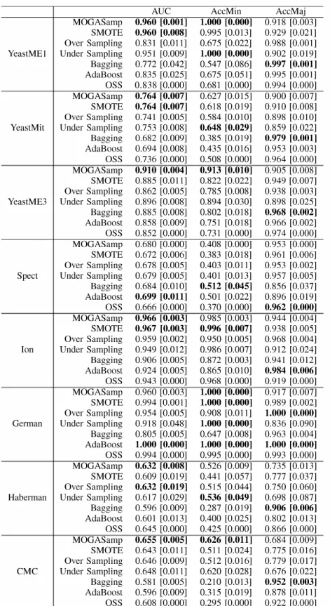
Table II shows the AVC, True Positive rate (minority class) and True Negative rate (Majority class) values obtained by the evaluated techniques in each data set used. The values presented are the mean and standard deviation after running 30 times each algorithm. We highlight in bold the highest value for each measure.
In order to statistically validate the obtained results, we present the results of statistical tests by following the approach proposed by Demsar [29]. In brief, this approach seeks to com pare multiple algorithms on multiple data sets, and it is based on the use of the Friedman test with a corresponding post hoc test. The Friedman test is a non-parametric counterpart of the well-known ANOVA. If the null hypothesis, which states that the classifiers under study present similar performances, is rejected, then we proceed with the Nemenyi post-hoc test for pairwise comparisons.
The results suggest that MOGASamp achieved the best overall performance. The ranking provided by the Friedman test supports this assumption, showing MOGASamp as the best-ranked method on AVC and True Positive rate and sixth best-ranked method on True Negative rate. The Friedman test also indicates the rejection of the null hypothesis, confirming that the differences among the algorithms are statistically significant (AVC: p-value = 0.0071, AccMin: p-value =
2.74 x 10⁻⁵, AccMaj: p-value = 9.40 x 10⁻⁵). Hence, we have
executed the Nemenyi post-hoc test for the purpose of pairwise comparison. The proposed method outperforms the Bagging and OSS on True Positive rate and outperforms the Bagging on AVC with statistical significance at a 95% confidence level. AVC was used as a measure for evaluating the performance of each approach considering both classes. It can be seen that
AVC AccMin AccMaj
MOGASamp 0.960 [0.001] 1.000 [0.000] 0.918 [0.003]
SMOTE 0.960 [0.008] 0.995 [0.013] 0.929 [0.021] Over Sampling 0.831 [0.011] 0.675 [0.022] 0.988 [0.001] YeastMEl Under Sampling 0.951 [0.009] 1.000 [0.000] 0.902 [0.019] Bagging 0.772 [0.042] 0.547 [0.086] 0.997 [0.001] AdaBoost 0.835 [0.025] 0.675 [0.051] 0.995 [0.001] OSS 0.838 [0.000] 0.681 [0.000] 0.994 [0.000] MOGASamp 0.764 [0.007] 0.627 [0.015] 0.900 [0.007] SMOTE 0.764 [0.007] 0.618 [0.019] 0.910 [0.008] Over Sampling 0.741 [0.005] 0.584 [0.010] 0.898 [0.010] YeastMit Under Sampling 0.753 [0.008] 0.648 [0.029] 0.859 [0.022] Bagging 0.682 [0.009] 0.385 [0.019] 0.979 [0.001] AdaBoost 0.694 [0.008] 0.435 [0.016] 0.953 [0.003] OSS 0.736 [0.000] 0.508 [0.000] 0.964 [0.000] MOGASamp 0.910 [0.004] 0.913 [0.010] 0.905 [0.008] SMOTE 0.885 [0.011] 0.822 [0.022] 0.949 [0.007] Over Sampling 0.862 [0.005] 0.785 [0.008] 0.938 [0.003] YeastME3 Under Sampling 0.896 [0.008] 0.894 [0.030] 0.898 [0.025] Bagging 0.885 [0.008] 0.802 [0.018] 0.968 [0.002] AdaBoost 0.858 [0.009] 0.751 [0.018] 0.966 [0.002] OSS 0.852 [0.000] 0.731 [0.000] 0.974 [0.000] MOGASamp 0.680 [0.000] 0.408 [0.000] 0.953 [0.000] SMOTE 0.672 [0.006] 0.383 [0.018] 0.961 [0.006] Over Sampling 0.678 [0.005] 0.403 [0.011] 0.953 [0.002] Spect Under Sampling 0.679 [0.005] 0.401 [0.013] 0.957 [0.005] Bagging 0.684 [0.010] 0.512 [0.045] 0.856 [0.037] AdaBoost 0.699 [0.011] 0.501 [0.022] 0.896 [0.019] OSS 0.666 [0.000] 0.370 [0.000] 0.962 [0.000] MOGASamp 0.966 [0.003] 0.985 [0.003] 0.944 [0.004] SMOTE 0.967 [0.003] 0.996 [0.007] 0.938 [0.005] Over Sampling 0.959 [0.002] 0.950 [0.005] 0.968 [0.004]
Ion Under Sampling 0.949 [0.012] 0.986 [0.007] 0.912 [0.024]
Bagging 0.906 [0.005] 0.872 [0.003] 0.941 [0.012] AdaBoost 0.924 [0.005] 0.865 [0.010] 0.984 [0.006] OSS 0.943 [0.000] 0.968 [0.000] 0.919 [0.000] MOGASamp 0.960 [0.003] 1.000 [0.000] 0.917 [0.007] SMOTE 0.994 [0.001] 1.000 [0.000] 0.989 [0.002] Over Sampling 0.954 [0.005] 0.908 [0.011] 1.000 [0.000]
German Under Sampling 0.918 [0.048] 1.000 [0.000] 0.836 [0.090] Bagging 0.805 [0.005] 0.647 [0.008] 0.963 [0.004] AdaBoost 1.000 [0.000] 1.000 [0.000] 1.000 [0.000] OSS 0.994 [0.000] 0.995 [0.000] 0.993 [0.000] MOGASamp 0.632 [0.008] 0.526 [0.009] 0.735 [0.013] SMOTE 0.609 [0.019] 0.441 [0.057] 0.777 [0.037] Over Sampling 0.632 [0.019] 0.515 [0.044] 0.750 [0.060] Haberman Under Sampling 0.617 [0.029] 0.536 [0.049] 0.698 [0.087] Bagging 0.596 [0.009] 0.287 [0.019] 0.906 [0.006] AdaBoost 0.601 [0.013] 0.400 [0.025] 0.802 [0.013] OSS 0.645 [0.000] 0.425 [0.000] 0.866 [0.000] MOGASamp 0.655 [0.005] 0.626 [0.011] 0.684 [0.009] SMOTE 0.643 [0.011] 0.511 [0.024] 0.775 [0.016] Over Sampling 0.646 [0.009] 0.512 [0.016] 0.779 [0.017] CMC Under Sampling 0.648 [0.011] 0.620 [0.028] 0.676 [0.022] Bagging 0.581 [0.005] 0.210 [0.013] 0.952 [0.003] AdaBoost 0.596 [0.009] 0.315 [0.019] 0.878 [0.011] OSS 0.608 [0.000] 0.295 [0.000] 0.922 [0.000]
TABLE II: AUe and classification accuracy of the Minority and Majority classes (average and standard deviation) using different resampling and classification techniques
MOGASamp presented the best values in six of the data sets, and in the data set Ion it achieved a performance statistically similar to that of SMOTE. Another important aspect to be highlighted is that the proposed method did not present the
worst AUe value in any of the evaluated data sets. This is an indication that MOGASamp can be applied to different data sets with different imbalance ratio, even without a priori knowledge.
As discussed previously, an effective way to evaluate a classifier with imbalanced data is using the rates of classifica tion errors made in each class, since traditional classification algorithms tend to favor the majority class rather than the minority class. Based on this fact, it can be seen in Table II that the proposed method presented a trade-off between the rates of True Positives and True Negatives.
Analyzing the true positive values, MOGASamp achieved the best results in four data sets. In fact, considering the data sets YeastME3 and CMC, MOGASamp presented the highest values in experimental tests. These results were obtained without sacrificing the accuracy of the majority class (True Negative rate). The undersampling technique achieved good True Positive values, albeit it presented low True Negative values.
When analyzing the True Negative rate values, one can observe that Bagging presents significant results. However, Bagging does not present good values for True Positive rate. This fact indicates that this method does not have a good performance when dealing with imbalanced data. The main reason of this drawback is the fact that Bagging, as well as other classical classification algorithms, assumes that the data is balanced, then giving preference to the majority class. Similar situation can be observed in the AdaBoost and OSS methods.
VI. CONCLUSION
In this paper, we presented a new evolutionary approach, called MOGASamp (Multiobjective Genetic Sampling), to address the problem of classification with imbalanced data sets. This approach is based on a multiobjective genetic algorithm. It uses two metrics AVC and PFC to evolve a set of balanced samples of the training data set, until a set of classifiers with high accuracy and diversity is reached. The obtained classifiers are used as an ensemble of classifiers to predict new instances using majority voting.
Experimental tests were performed using eight data sets and the obtained results were compared with well known resampling and classification techniques from the literature. The experimental results has shown that MOGASamp presents high predictive accuracy, obtaining better results in six of the data sets. Furthermore, MOGASamp has also shown high stability to predict the data of both classes. This means that MOGASamp does not show noticeable differences in the rate of True Positives and True Negatives, which is the main draw back of classical algorithms when dealing with imbalanced data.
ACKNOWLEDGMENT
The authors would like to thank FAPESP, CAPES and CNPq for their financial support.
REFERENCES
[1] A. 1. Marques, V. Garcia, and J. S. Sanchez, "On the suitability of resampling techniques for the class imbalance problem in credit scoring," Journal of the Operational Research Society, vol. 64, no. 7, pp. 1060-1070, 2013.
[2] H. He and E. A. Garcia, "Learning from imbalanced data," IEEE Transactions on Knowledge and Data Engineering, vol. 21, no. 9, pp. 1263-1284, 2009.
[3] Z.-H. Zhou, "Ensemble learning." in Encyclopedia of Biometrics, S. Z. Li and A. K. Jain, Eds. Springer US, 2009, pp. 270-273.
[4] K. Turner and J. Ghosh, "Analysis of decision boundaries in linearly combined neural classifiers," Pattern Recognition, vol. 29, pp. 341-348, 1996.
[5] T. G. Dietterich, "Machine-learning research - four current directions,"
AI Magazine, vol. 18, pp. 97-136, 1997.
[6] A. Krogh and J. Vedelsby, "Neural network ensembles, cross validation, and active learning," in Advances in Neural Information P rocessing Systems. MIT Press, 1995, pp. 231-238.
[7] A. Chandra and X. Yao, "Ensemble learning using multi-objective evolutionary algorithms," 1. Math. Mode!. Algorithms, vol. 5, no. 4, pp. 417-445, 2006.
[8] Y. Liu and X. Yao, "Negatively correlated neural networks can produce best ensembles," Australian Journal of Intelligent Information P rocess ing Systems, vol. 4, no. 3/4, pp. 176-185, 1997.
[9] A. Chandra and X. Yao, "DIVACE: diverse and accurate ensemble learning algorithm," in Intelligent Data Engineering and Automated Learning - IDEAL 2004. 5th International Conference. Exeter, UK. August 25-27. 2004. Proceedings, 2004, pp. 619-625.
[10] T. Deepa and M. Punithavalli, "An analysis for mining imbalanced datasets;' International Journal of Computer Science and Information Security, vol. 8, pp. 132-137, 2010.
[11] B. Zadrozny, J. Langford, and N. Abe, "Cost-sensitive learning by cost proportionate example weighting," in P roceedings of the Third IEEE International Conference on Data Mining, ser. ICDM '03. IEEE Computer Society, 2003, pp. 435-442.
[12] M. Kubat and S. Matwin, "Addressing the curse of imbalanced training sets: One-sided selection," in In Proceedings of the Fourteenth Inter national Conference on Machine Learning. Morgan Kaufmann, 1997, pp. 179-186.
[13] P. E. Hart, 'The condensed nearest neighbor rule (corresp.)." IEEE Transactions on Information Theory, vol. 14, no. 3, pp. 515-516, 1968. [14] Y. Sun, A. K. C. Wong, and M. S. Kamel, "Classification of imbalanced data: a review," International Journal of Pattern Recognition and Artificial Intelligence, vol. 23, no. 4, pp. 687-719, 2009.
[15] R. C. Holte, L. Acker, and B. W. Porter, "Concept learning and the problem of small disjuncts." in IJCAI, N. S. Sridharan, Ed. Morgan Kaufmann, 1989, pp. 813-818.
[16] N. V. Chawla, K. W. Bowyer, L. O. Hall, and W. P. Kegelmeyer, "Smote: Synthetic minority over-sampling technique," Journal of Artificial In telligence Research, vol. 16, pp. 321-357, 2002.
[17] V. Garca, A. I. Marqus, and J. S. Snchez, "Improving risk predictions by preprocessing imbalanced credit data." in ICONIP (2), ser. Lecture Notes in Computer Science, T. Huang, Z. Zeng, C. Li, and c.-S. Leung, Eds., vol. 7664. Springer, 2012, pp. 68-75.
[18] L. Breiman and L. Breiman, "Bagging predictors," in Machine Learn ing, 1996, pp. 123-140.
[19] Y. Freund and R. E. Schapire, "A decision-theoretic generalization of on-line learning and an application to boosting," 1. Comput. Syst. Sci.,
vol. 55, no. I, pp. 119-139, Aug. 1997.
[20] A. P. Bradley, "The use of the area under the roc curve in the evaluation of machine learning algorithms," Pattern Recognition, vol. 30, pp. 1145-1159, 1997.
[21] F. J. Provost and T. Fawcett, "Analysis and visualization of classifier performance: Comparison under imprecise class and cost distributions." in KDD, D. Heckerman, H. Mannila, and D. Pregibon, Eds., 1997, pp. 43-48.
[22] L. 1. Kuncheva, Combining Pattern Classifiers: Methods and Algo rithms. Wiley-Interscience, 2004.
[23] K. Deb, A. Pratap, S. Agarwal, and T. Meyarivan, "A fast and elitist multi objective genetic algorithm: NSGA-II," Trans. Evo!. Comp, vol. 6, no. 2, pp. 182-197, Apr. 2002.
[24] K. Deb, Multi-Objective Optimization using Evolutionary Algorithms,
ser. Wiley-Interscience Series in Systems and Optimization. John Wiley
& Sons, Chichester, 2001.
[25] K. Bache and M. Lichman, "UCI machine learning repository," 2013. [Online]. Available: http://archive.ics.uci.edu/ml
[26] L. Torgo, "DMwR: Functions and data mining with R" " 2010. [Online]. Available: project.orglbinlwindows/contrib/3 .3/DMwR_O A.l.zip [27] A. D. Pozzolo, O. Caelen, and G. Bontempi,
The package implements different data-driven unbalanced datasets," 2014. [Online]. Available: project.orglbinlwindows/contrib/3.3/unbalanced_l.l.zip for "data http://cran.r-"unbalanced: method for http://cran.r-[28] E. Alfaro, M. Gamez, and N. Garcia, "adabag: An R package for classification with boosting and bagging," pp. 1-35, 2013. [Online]. Available: http://www.jstatsoft.org/v54/i02/
[29] J. Demsar, "Statistical comparisons of classifiers over multiple data sets," 1. Mach. Learn. Res., vol. 7, pp. 1-30, Dec. 2006.