Default Predictors and Credit Scoring Models for Retail Banking

Default Predictors and Credit Scoring Models

for Retail Banking

Evžen Kočenda

Martin Vojtek

CES

IFO

W

ORKING

P

APER

N

O

.

2862

C

12:

E

T

M

D

2009

An electronic version of the paper may be downloaded

• from the SSRN website: www.SSRN.com

• from the RePEc website: www.RePEc.org

CESifo Working Paper No. 2862

Default Predictors and Credit Scoring Models

for Retail Banking

Abstract

This paper develops a specification of the credit scoring model with high discriminatory power to analyze data on loans at the retail banking market. Parametric and non- parametric approaches are employed to produce three models using logistic regression (parametric) and one model using Classification and Regression Trees (CART, nonparametric). The models are compared in terms of efficiency and power to discriminate between low and high risk clients by employing data from a new European Union economy. We are able to detect the most important characteristics of default behavior: the amount of resources the client has, the level of education, marital status, the purpose of the loan, and the number of years the client has had an account with the bank. Both methods are robust: they found similar variables as determinants. We therefore show that parametric as well as non-parametric methods can produce successful models. We are able to obtain similar results even when excluding a key financial variable (amount of own resources). The policy conclusion is that socio-demographic variables are important in the process of granting credit and therefore such variables should not be excluded from credit scoring model specification.

JEL Code: B41, C14, D81, G21, P43.

Keywords: credit scoring, discrimination analysis, banking sector, pattern recognition, retail loans, CART, European Union.

Evžen Kočenda

Charles University and the Academy of Sciences (CERGE-EI) P.O. Box 882 Politických vĕzňů 7 111 21 Prague Czech Republic [email protected] Martin Vojtek Czech National Bank

Na Příkopĕ 28 115 03 Prague Czech Republic [email protected]

We would like to thank Martin Čihák, Jarko Fidrmuc, Christa Hainz, Stefanie Kleimeier, Filip Palda, Hendrik Wagner, and an anonymous referee for helpful comments. GAČR grant support (402/09/1595 and 402/05/0931) is gratefully acknowledged. The usual disclaimer applies.

1. Introduction

Despite the wide variety of banking services, lending to corporate clients and the public still constitutes the core of the income of commercial banks and other lending institutions. Due to asymmetric information, lending carries a risk in terms of defaulted loans. Hasan and Zazzara (2006) stress that under the new Basel II rules that are grounded in recognizing an individual credit risk through internal rating systems, banks’ managers must correctly measure risk and price it accordingly. Credit scoring greatly reduces the risk provided a capable model is applied and reliable data are available as firmly shown by Dinh and Kleimeier (2007).

Following the above arguments we build two parametric and one non-parametric credit scoring models and test them on a large dataset of retail loans containing financial as well as behavioral and socio-demographic variables from a new EU economy.1 Based on various tests as well as out-of-sample testing we show that our models deliver efficient results in terms of potential default identification and that socio-demographic data are useful predictors of future characteristics relevant to the loan granting process. This is certainly good news as the findings of Jacobson, Lindé and Roszbach (2005) show that retail portfolios are usually riskier than corporate credit.2 In our paper we contribute to the literature by providing insights about the main determinants of risk in the retail credit market by using two different methodologies.

1.1. Literature

From a technical perspective, the lending process is a relatively straightforward series of actions involving two principal parties. These actions go from the initial loan application to the successful repayment of the loan or its default. Although retail lending is among the most profitable investments in lenders' asset portfolios (at least in developed countries), increases in the amount of loans also bring increases in the number of defaulted loans. Thus, the primary problem of any lender is to differentiate between “low

1

We did not incorporate macroeconomic variables into our analysis, as our main area of interest was to focus on socio-demographic variables. Also, our data sample reflects only a period of steady macroenomic growth in the Czech Republic and to estimate the impact of macroeconomic developments on individual defaults would require at least whole economic cycle.

2

The models developed in this paper may not be transferable to banking markets in the other new EU member countries due to the specificity of the data used. Each bank has its own processes and ways to deal with clients and defaulted credits and therefore models used in the respective bank may be highly specific.

risk” and “high risk” debtors prior to granting credit. Due to the asymmetric information between the lender and borrower such differentiation is not a trivial task. However, it is possible by using parametric or non-parametric credit-scoring methods.

The practice of credit scoring began in the 1960's, when the credit card business matured and automatic decision-making processes became necessary. Later, the use of credit scoring techniques was extended to other classes of customers, in particular to small and medium enterprises. In this respect, Myers and Forgy (1963) compared discrimination analysis with regression in credit scoring applications and Beaver (1967) introduced a bankruptcy prediction model. The two works above both focused on two aspects: predictions of failure as well as on the classification of credit quality. This is an important distinction in empirical analysis as it is often not clear which aspect to focus on. Altman (1980) described the basic bank lending process as an integrated system and analyzed a procedure for how the criteria for the assessment of commercial loans is set.3

Most of the credit-scoring literature deals with non-retail loans, i.e. loans to firms, as the data are more readily available. Corporate credit scoring—also known as rating assignment—is different from scoring for retail loans for several reasons. Primarily, the amounts lent are much smaller in the case of retail lending, and therefore from the point of view of risk management, retail loans are dealt with using a portfolio approach, while corporate loans are managed on an individual basis. Most importantly, there are different types of variables used in the process of constructing a model as well as the decision process for each type of loan. For example, for corporate loans, various ratios of financial indicators are typically used in corporate failure models since they are usually very powerful in determining the quality of a client.4 As regards collateral, for example Blazy and Weill (2006) state that it might be that riskier loans are more likely to be collateralized, otherwise these projects would not be financed. In retail lending, the bank has to collect various socio-demographic characteristics, as well as various behavioral indicators (e.g. indicators of a client’s behavior on his current account) to make a decision about the client’s portfolio.

3

For a more thorough exposition of the credit scoring literature, see Renault and De Servigny (2004).

4

As an example of early methodologies concerning retail loans, Long (1976) studied a selection of the empirically best credit scoring techniques and proposed criteria for the optimal updating cycle of a credit scoring system. Apilado, Warner and Dauten (1974) empirically studied two hypotheses: that there is a limited set of variables discriminating between low and high risk loans with a high degree of accuracy and that profitability can be increased without increasing risk for most lenders. Gropp et al. (1997) examined how personal bankruptcy and personal bankruptcy exemptions affect the supply of and demand for credit. They found that bankruptcy exemptions redistribute credit towards borrowers with a high level of assets. As an example of recent work in the area of retail credit scoring, Avery et al. (2004) examine the potential costs of failing to incorporate into consumer credit evaluations situational data, such as information about the economic or personal circumstances of individuals. They also discuss practical difficulties associated with the development of credit scoring models that incorporate situational data. For further examples of the uses of credit scoring in retail banking see Jacobson and Roszbach (2003); Allen, DeLong, and Saunders (2004); Wagner (2004); Jacobson, Lindé and Roszbach (2005); Bofondi and Lotti (2006); Dinh and Kleimeier (2007); and Saurina and Trucharte (2007). Finally, Hand and Henley (1997) provide an excellent survey of the statistical techniques used in the process of building a credit scoring model.

1.2 Objective

In this paper we focus on an analysis of the determinants of defaults of retail loans in a new EU economy (the Czech Republic). New EU members have recently recorded a sharp increase in the amount of this type of loan, and the increase is expected to continue. Hilbers et al. (2005) review trends in bank lending to the private sector, with a particular focus on Central and Eastern European countries, and find that the rapid growth of private sector credit may create a key challenge for most of these countries in the future. Take for example two countries on the forefront of the EU integration process: in the last few years, banks in the Czech Republic and Slovakia have allocated a significant part of their lending to retail clientele. Even before the integration of both countries into the EU, the financial liabilities of households between years 1999–2004 (which is covered by our data) increased more than twice in both countries (relative to GDP). Later on, in 2006,

Czech and Slovak banks recorded 30.5% and 32% increases in retail loans, respectively. In 2007 these increases amounted to 35.2% and 27.8%, respectively. In the Czech Republic and Slovakia the financial liabilities of households formed 15.6% and 15.7%, respectively, of the GDP in 2006. In 2007 these liabilities increased to 18.8% and 16.4%, respectively.5 The average ratio of financial liabilities to GDP in the older 15 members of the European Union is about three times higher than in the Czech Republic and Slovakia;6 it is expected that the amount of loans to retail clientele will continue to increase, as there is a lot of space for expansion in the financial liabilities of households in both countries (even though the household sectors in at least some of the older EU countries clearly took on too much debt).

In light of these recent developments, we address the primary problem of lenders: how to determine between low and high risk debtors prior to granting credit. That means we aim to build an application type of model that would primarily be suitable for the pre-scoring of clients.7 One of our goals is to look at the importance of socio-demographic variables as determinants of default. The reason is that this type of variable provides useful information in times of change. This is particularly true in new EU members that recently underwent an unprecedented economic transformation and have integrated into the EU. Socio-demographic variables evolve in a stable manner over time and a well-designed credit scoring model based on socio-demographic and behavioral variables might perform as well as a model based on historic or current financial characteristics.

In this paper we contribute to the literature in several ways. First, we construct two types of credit scoring model, one based on logistic regression and the other on Classification and Regression Trees (CART). Both methods are often used for developed countries and we are interested in whether they are able to construct a powerful credit scoring model for new EU markets that due to their economic history differ from the old

5

These numbers, which originate from the financial stability reports of the central banks of both countries, cover only the banking sector and not other types of lending institutions.

6

As of 2006; source: EU economic data pocketbook.

7

The models constructed in this paper are not appropriate for example for the ongoing and regular calculation of regulatory capital as they rely mostly on the application characteristics of clients valid at the time of loan application. Application characteristics are usually not updated during the life of the loan and they grow more imprecise as time elapses and therefore are not suitable for the assessment of the current riskiness of a portfolio of bank loans. Also, as our main concern is the probability of default models, we do not take into account the loss given default parameter of defaulted loans.

EU members. Second, we test our models on an empirical dataset from one of the banks operating in the retail loan business in a new EU market (the Czech Republic). Based on out-of-sample testing we compare the efficiency of the two methods and identify the key determinants of default behavior, with socio-demographic variables being important.8 We show that with the logistic regression model we were able to build a specification that does not contain the single most important financial variable (available resources) but still performs only marginally worse than the specification with this variable.

The rest of the paper is organized as follows. In Section 2 we describe the data used in the estimation process. Section 3 describes the empirical methodology and results and Section 4 concludes.

2. Data

In this section we briefly introduce our dataset. We intentionally deviate from standard practice and introduce our data prior to describing the models. This helps us describe our models in a more lucid way. Some details about the data are also introduced in the model section, where they fit more naturally.

The dataset used for the estimation in this paper comes from a new EU member (the Czech Republic) and was provided by a bank that specializes in providing small- and medium-sized loans to retail clientele in the area of real property purchase and reconstruction.9 The same data have been used for the bank’s own assessment and scoring modeling. The dataset contains various socio-demographic characteristics and other information collected by the bank on 3403 individual clients who were granted loans during 1999–2004. The observation period ends in 2006. Out of these, 1695 clients defaulted on loans and 1708 performed well, i.e. the sample is artificially balanced to have approximately 50% of defaults. The loans are evenly distributed during the analyzed

8

To the best of our knowledge, the empirical studies analyzing this type of problem, with emphasis placed on credit scoring related to retail loans, are non-existent in post-transition countries that became EU members. Part of the lack is due to the fact that commercial banks in post-transition EU countries, especially the biggest ones, are not willing to share their credit-related data. This is understandable since having datasets connected with the default behavior of retail clients can be a competitive advantage over other banks because these datasets enable the bank to construct better credit models. A bank with an accurate and powerful credit scoring model not only decreases its costs connected with bad loans, but also strengthens a bank’s risk management in general.

9

The bank does not wish to be explicitly identified and we honor this request as specified in the contract to provide us with the data.

period. There is no concentration of defaults in any period. Each individual client had no more than one loan, so there was no need to aggregate several loans for one individual, as is often the case for companies. The definition of default follows the Bank for International Settlement standard: the client is in default if he or she is more than 90 days overdue with any payment connected with the loan. The definition of a good/bad variable is derived based on the performance of the client, i.e. the client is considered “bad” in the case of his/her default.10 What follows in the next paragraphs is the economic motivation for including the various variables.

For all clients we have a number of variables that we present in Table 1 along with the variable definitions and whether they are categorized or continuous. The first part of the characteristics are socio-demographic variables and they characterize the client at the moment of loan application. Among others, there are several categorized variables related to the client’s employment situation. The bank does not record information about the client’s income and expenditures; instead the bank calculates and records the relevant credit ratios. The first ratio is the percentage of income that is spent on expenditures (Credit Ratio 1). The second ratio is the ratio of a client’s available income to the official minimum wage valid at the time of the loan application (Credit Ratio 2). The client’s region is designated by the postal code of the region of the client’s address.

The other part of the variables characterizes the relationship between the client and the bank. The Loan Protection variable records the credit risk mitigation used, i.e. whether collateral, a guarantor or another type of mitigation was used. It is important to take into account collateral or guarantee of loan as a riskier but well-collateralized loan may be more profitable for a bank than a somewhat less risky loan without collateral. The Points variable is the only behavioral characteristic available.11 It is a variable

10

The bad/good notion is an official definition taken from the Basel II descriptive characteristics of a client or her/his loan after the loan has been granted and the bank can see the client’s performance with respect to the loan.

11

Behavioral characteristics are very powerful indicators of the type of client. However, the client needs to have a history with the bank in order to use these indicators. Hence, we do not possess other behavioral variables such as delinquency. A new client has to be scored almost solely on the basis of her/his socio-demographic characteristics (as there is still no individual public credit ratings in the Czech Republic that banks can use to inform themselves). This is also the reason why we do not take into account the bank’s interest rate setting policy.

constructed by the bank and describes the client’s behavior on his or her own current account. It quantifies the frequency at which the client deposits money into the account as well as whether the deposits follow a regular pattern. Hence, the Points variable depends on the amount of a client’s savings as well as on how regular saving deposits are made. The Own Resources variable is the amount of resources the client declares to have at the time of loan application available to use for the purpose defined in the Purpose of Loan variable. For example, it can be the amount of money a client can allocate as a down payment for the purchase of an apartment. The Length of Relationship variable is the number of years between when the loan was granted and when the client opened an account with the bank.12 We have also tested the sample for the possible multicollinearity of the Length of Relationship variable and the Date of Account Opening, but found no significant results.

Finally, our data sample contains information about borrowers who were eventually granted loans and does not contain information on rejected applicants, i.e. clients who applied for credit but were rejected, as the bank did not collect this data. The true creditworthiness status of the rejected applicants is unknown and their characteristics might differ from those who were granted a loan. For this reason a potential selection bias may occur in our estimations. This is a common problem in the literature and we assume that other potential borrowers have similar characteristics as those in the database. In addition, Banasik, Crook and Thomas (2003) compared the classification accuracy of a model based only on accepted applicants relative to one based on a sample of all applicants, and found only a minimal difference. Further, Hand and Henley (1993) analyze a “reject inference” process, i.e. a process of attempting to infer the true creditworthiness status of rejected applicants. They concluded that a reliable rejection inference is impossible and improvements in scoring models achieved by reject inference are based on luck, the use of additional information (for example using expert skill) or ad hoc adjustments of the rules in a direction likely to lead to a reduced bias.

3. Estimation techniques

12

The Date of Loan variable is an endogenous variable and it is not possible to discriminate on the basis of this variable. Therefore this variable is not used in the subsequent analysis.

In this section we introduce two distinct techniques for credit scoring. These are a parametric approach with a logistic regression and a non-parametric Classification and Regression Trees (CART) model. The methods are described in Sections 3.1. and 3.2, respectively.

As it is not practical to use more than 20 variables in logistic regression or in the process of creating trees, single factor analysis was performed as the first step of the estimation. With single factor analysis we tried to eliminate variables which have no discriminating power. We calculated the so-called “odds ratio” and “information value” for each variable. Both characteristics show the degree of the ability of the variable to discriminate between defaulted and non-defaulted loans. Variables with the lowest information values were then omitted.

The odds ratio can be used to determine the discrimination ability of the variable for the given category. It is defined as

⎟ ⎠ ⎞ ⎜ ⎝ ⎛ ⎟ ⎠ ⎞ ⎜ ⎝ ⎛ = i i i Good Good Defaulted Defaulted Odds ,

where Defaulted and Good are the total numbers of defaulted and non-defaulted observations and Defaultedi and Goodi are the numbers of defaulted and non-defaulted

clients in the ith category of a variable. An odds ratio equal to 1 implies that the variable is not able to discriminate between defaulted and non-defaulted clients in the given category; other values signal the discrimination ability of the variable.

The overall information value of a variable is the sum of the information values for each category of variable, which are defined as

⎟⎟ ⎠ ⎞ ⎜⎜ ⎝ ⎛ − = Good Good Defaulted Defaulted Odds IV i i i i ln( ) .

This information value symbolizes the predictive power of the variable: the higher the value, the higher the predictive power of the variable with the given categorization. In banking practice a value above 0.2 is taken as a sign of the strong predictability of a given variable.

For our analysis we decided to categorize the continuous variables. Although it is possible to build a model using both continuous and discrete variables, the standard practice in credit scoring is to use categorized continuous variables. We used the

following practice.13 First, the range of values for each continuous variable was split into ten categories according to the following two principles:

1. All categories should have the same number of observations, with one exception. 2. The exception is that observations with the same value for the specific variable have to be in the same category.

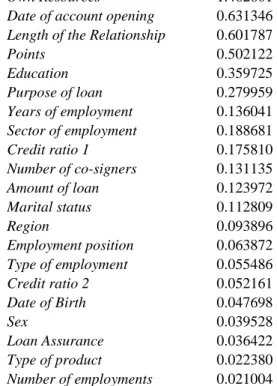
The odds ratios and information values were calculated for each category and categories with similar values were merged. This step was also performed for the categorized variables. The odds ratios and information values for the categories of variables from the sample can be found in the Appendix (Table A1). The total information values for the variables can be found in Table 2. It can be seen that the most significant variables are those that characterize the relationship between the client and the bank, a finding that is in accord with the comprehensive overview in Anderson (2007). The variables that characterize the loan protection and credit quality of the debtor (i.e. both credit ratios) are almost insignificant. This fact is surprising especially in the case of loan protection as one would expect that collateral in the form of real estate would be an effective predictor of good performance. However, this detail can be explained by the fact that the amount of each loan in the data sample is not excessively large and therefore even a defaulted loan does not necessarily result in a loss of property.

It is also interesting that most of the socio-demographic variables are not significant. Only Education is a very strong default predictor since clients with a higher level of education show much less default than other clients. Marital Status, Region, Sex and Employment Position have low information values.14 Another interesting factor is the difference in the information value of both credit ratios. It seems that the default behavior of clients does not depend on the absolute amount of “savings” (i.e. the difference between income and expenditures) but on relative income (i.e. the ratio of expenditures to income). In other words, even high income clients who also have high expenditures can be risky clients.

13

There are also other ways to categorize continuous variables, see for example Wermuth and Cox (1998).

14

The low information value of the Sex variable is in contrast to finding in Dinh and Kleimeier (2007), where Sex/Gender was found to have good predicting power, as micro finance literature suggest that women repay more reliably. The low information value of the Sex variable also hints at non-discriminatory practices, which are otherwise documented for example by Alesina (2009) in Italy.

We will proceed now with the two discrimination techniques to analyze the determinants of default behavior. In the course of this analysis we will also compare logistic regression with CART (Classification and Regression Trees).

3.1 Logistic regression

The theoretical background for using logistic, or logit, regression for classification in credit scoring has been outlined in the literature, and the literature also shows that logistic regression is usually very successful in determining low and high risk loans in tasks similar to ours. For details see for example Gardner and Mills (1989), Lawrence and Arshadi (1995), Hand and Henley (1997) or Charitou, Neophytou and Charalambous (2004).

In our analysis we decided to employ all variables with an information value higher than 0.1. The reason for such low threshold is to begin with employing more variables available for the logistic regression and also to have more socio-demographic variables, despite the fact that in our case these tend to exhibit lower information values. Although there are missing values in several of the variables, this problem was eliminated by categorization, i.e. by creating a category for the missing values. We employed forward-backward stepwise model selection using Akaike Information Criterion (AIC) to select the best model. Logistic regression usually starts with the simplest model, i.e. with a regression on a constant only. After each step, the chosen model is tested and a decision is made on whether any variable can be left out based on the change in the value of the information criterion. Then all the models that differ from the current one by adding a single variable are tested. This procedure should choose the best model among all the models based on the supplied regressors (variables). The coefficients are estimated using the maximum likelihood method. Statistical analysis was performed using S-PLUS 6.2 software.

In order to evaluate the performance of our models we follow a strategy to partition our dataset into two samples: one for development (development sample) and one for validation purposes (validation sample). This way an out-of-sample validation can be performed. The dataset was randomly split such that the development sample contains two-thirds of the observations (2280 observations) and the validation sample

contains one-third of the observations (1143 observations). The validation sample will be later used to test the discriminatory power of the model on a sample that was not used in the development stage of the model (out-of-sample testing). The validation sample uses different observations as well as different borrowers than those used in the estimation sample.

The quality of the models is tested using the Receiver Operating Curve (ROC) and the GINI coefficient. Webb (2002) defines the ROC as the plot of the true positive rate on the vertical axis against the false positive rate on the horizontal axis. All the ROC curves pass through the (0,0) and (1,1) points and as the separation increases the curve moves into the top left corner. The ideal model should perform 100% detection and have a 0% false positive rate. The ROC in the case of the ideal model is characterized by a kinked curve passing through the coordinates (0,0)-(0,1)-(1,1). Different models produce different ROCs, characterizing the performance of the model. The performance is defined as the area under the curve and is usually denoted as the c coefficient. It follows that the ideal model has an area under the curve c=1. For the GINI coefficient g, which is the area under the Lorenz curve, the relationship g = 2c - 1 is valid.

However the choice of the model in practice does not always depend only on the ROC curve and the GINI coefficient. It may be important to look at the Type I error (accepting a bad loan as a good loan) and Type II error (rejecting a good loan as a bad loan). It is a generally-accepted fact the misclassification costs of a Type I error are much higher than those of a Type II error. For a Type I error the lender may lose the whole amount of loan and its interest while for a Type II error it is only the expected profit from the loan. Therefore it may be important to look at the full curve not only at the parameter

c. In banking practice therefore the choice of model may be based on minimizing misclassification costs.

The logistic regression is based on the following idea. Given a vector of application characteristics x, the probability of default p is related to vector x by the relationship

∑

where coefficients wi represent the importance of specific loan application characteristic

coefficients xi in the logistic regression. Coefficients wi are obtained by using maximum

likelihood estimation. Logistic regression can handle categorized data by employing a dummy variable for each category in the data.

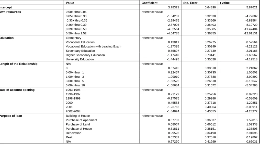
Using this method we first estimate Model 1, which is the output of the stepwise procedure; i.e. the model was selected as the ideal model using the above-mentioned forward and backward stepwise technique. The estimates are presented in Table 3, which also contains the list of variables used. The score for each client can be calculated by summing the respective coefficient values, where the coefficient has a value of 0 for “reference category”. This model has several drawbacks. First, there are variables that have insignificant coefficients. Second, due to the high number of categories and variables, the model has also high number of degrees of freedom, a property that can lead to serious over-learning.

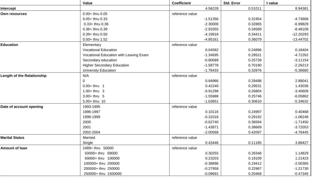
In Model 2 we eliminate variables with insignificant coefficients. In particular the following variables were dropped: Sector of Employment, Years of Employment, and Purpose of Loan. Results are presented in Table 4. The elimination of several variables is justified also by the fact that the decrease in AIC was very slow for the last variables that entered the model. In Model 2 the value of the AIC increased only by about 2% and also the properties of the coefficients are similar to those in Model 1. Thus, Model 2 is able to discriminate among clients with fewer variables.

Finally, we estimate Model 3. The need for the third and last logistic model is driven by the fact that the variable Own Resources is a very strong default predictor. Therefore it might be useful to investigate the properties of other variables, i.e. to try to construct the model without this variable and to compare what the ability of the model is without this strong predictor. Further, the amount of resources a client has is usually very hard to detect, especially if a client would have to declare other funds he or she has outside the bank. Therefore it might be interesting to see whether it is possible to discriminate successfully without the knowledge of what funds the customer has. Model 3 is constructed using the same list of variables as Model 1 but the variable Own Resources is omitted.15 The coefficients of this model are presented in Table 5 and reveal

15

that Model 3 is able to successfully discriminate among clients without a knowledge of the resources the client owns.16

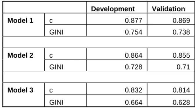
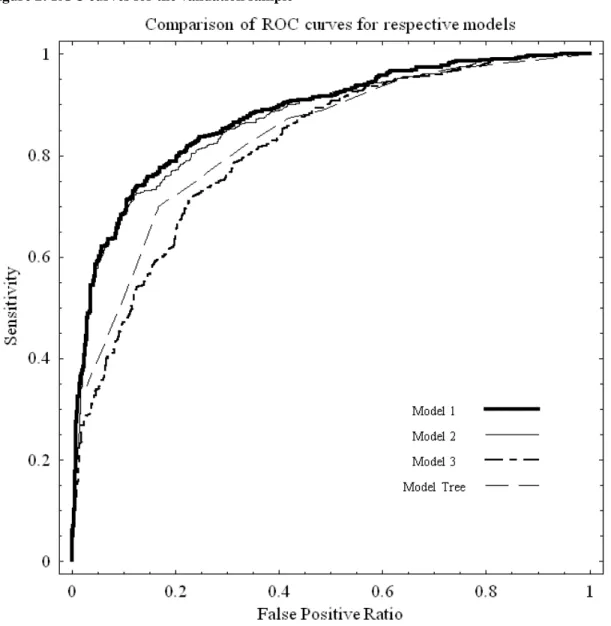
Next, we compare the quality of the three models using the Receiver Operating Curve (ROC) and c coefficients introduced earlier in this section. We plot the ROC curves (yielding also the c coefficient) on a single graph (Figure 1) so that a comparison of the empirical ROC curves resulting from the three logistic regression models is readily available.17 We can see that Models 1 and 2 are very similar in the shape of the ROC. They are also very close in terms of the derived values of the c coefficients: Model 1 has

c=0.877 and Model 2 has c=0.864, which is a difference of a mere 1.49%. That means that both models have very similar characteristics and are able to discriminate with almost the same power. Therefore Model 2 is preferred over Model 1 due to the principle of parsimony. Model 3 has a much higher value of the AIC, but more importantly the value of the c coefficient (c=0.832) is only marginally worse than that of Model 1 or 2. The consequences of this are striking: we do not need to know the variable Own Resources to construct a model with very similar power to a model containing this variable. This offers for example the possibility for a bank to check for fraud simply by running two different scoring functions: one which accounts for the declared resources the customer owns and one that does not. If there are serious differences in the results it may be worth examining the applicant further.

Another test of the power of a model is out-of-sample testing, i.e. the testing of the discriminatory power of the model on a sample that was not used in the development stage of the model, as we note in Section 1.1. In Table 6 we see the values of both c and the GINI statistics for all three models. It is possible to see that all models have similar power for both development and validation samples. As expected, Model 3 has lower power because the most important variable is left out. The approximately 11% loss of power does not seem that large in view of its great ability to discriminate in the absence of the single most important variable.

16

As a robustness check we also constructed a version of Model 3 using Model 2 with the variable Own Resources omitted. The results were equally strong as those presented in Table 5 for Model 3. Because of limited space we do not report detailed results, although they are available upon request.

17

In Figure 1 we also plot the empirical ROC from the Classification and Regression Trees (CART) methodology, whose results are presented in Section 3.2.

We also tested both constrained models (Models 2 and 3) versus Model 1 using the log-likelihood ratio test (LR test). The LR test is used in place of a standard F-test. The F-test, regularly used in the case of OLS regressions, cannot be employed because the response variable is not normally distributed. The LR test is performed by subtracting the so-called residual deviances of constrained and unconstrained models.18 The statistics has approximately a Chi-square distribution with n degrees of freedom, where n is the number of constraints. The null hypothesis is that the omitted variables are non-significant, i.e. their coefficients are equal to zero.

The residual deviances for all three models are: DEV1=2013.015,

DEV2=2104.823, and DEV3=2358.410. This means that when comparing Model 1 with

Model 2 the test statistics is LR12=91.808 with 23 degrees of freedom, and statistics

comparing Model 1 with Model 3 is LR13=345.395 with 17 degrees of freedom.19 The

values are highly statistically significant, implying that we should reject the null hypothesis of the non-significance of omitted variables. This is a sign that the omitted variables have statistical significance; however the power of all of the models is approximately the same. We conclude that all three models can be used for credit scoring. However, because of the high number of categories there is the risk connected with the possible over-learning of Model 1. Therefore, we lean towards Models 2 and 3. The final choice of the model should be based on other criteria dictated by special needs such as the results of the out-of-sample back-testing of models, requirements for model parsimony and data availability. Further, similarly to the condensed Figure 1 we also plot the out-of-sample ROC curves for all three models in Figure 2.20 A comparison of the out-of-sample ROC curves yields a similar outcome as in the case of the empirical ROC curves. Model 1 (c=0.869) and Model 2 (c=0.855) perform at a qualitatively similar level and Model 3 (c=0.814) lags only marginally behind.

Finally, despite the fact that it is common in the literature to use categorized data we also estimated specifications in which continuous variables were not categorized. As

18

The residual deviances are the analogue of the residual sum of squares in the OLS.

19

Such a high number of degrees of freedom is implied by the fact that each class of categorized variable adds one degree of freedom. Critical values at 1% are 41.638 and 33.409 for 23 and 17 degrees of freedom, respectively.

20

In accord with our previous approach, in Figure 2 we also plot the out-of-sample ROC from the CART methodology whose results are presented in Section 3.2.

one of our main goals is to construct a parsimonious model, we also tried a specification in which continuous variables are not categorized. In the case of the non-categorized data we need to estimate only one parameter for each continuous variable. This specification is also important as we are actually estimating a non-linear relationship with respect to these variables when we categorize them, because we allow for different sensitivity for different levels of the regressors. Therefore we are also interested in the power of the specification with variables that are not categorized.21 The power of the specification with non-categorized variables measured by the c coefficient was c=0.834, i.e. at a level comparable to that of the original Model 3. Hence, the results are less successful than those of the original Models 1 and 2. In the estimation we employed the same forward-backward stepwise model selection method as in the previous cases. The coefficients in the specification with non-categorized variables had similar signs as those for the original Model 1 (further confirming the robustness of the specification in our main model) with the most significant variable being Own Resources (with a coefficient value of -5.42117 and the t-value being -12.29606). Other variables chosen were Education, Purpose of Loan, Date of Account Opening, Marital Status, Length of Relationship with Bank, Sector and Years of Employment. The details associated with the above variables including their coefficients and t-values are reported in Table A2 in the Appendix.

We now turn to assessing and interpreting our results. With respect to the variable Own Resources, in both Model 1 and Model 2 it is possible to observe an inverse relationship between the amount of resources a client owns and the probability of default. Since we model the probability of default, a higher score reflects a higher default probability and, as one would expect, clients with more funds show a lower default probability.

Another strong predictor is Education Level, which shows that clients with a higher level of education have much less difficulty paying their debts. Clients with only general secondary education are riskier than those with vocational education at the secondary level who have passed the graduation examination.22 Frequently general

21

We acknowledge the referee for raising this issue.

22

Vocational education, also called career and technical education, prepares students for specific manual or practical careers. Vocational education can be at the secondary or post-secondary level. In some cases

secondary school graduates are not accepted for university education. People without specific vocational education and without a university education have a harder time getting better-paid job. They are also more likely to fail to find permanent employment and to become unemployed, and thus they more often fall into the lowest income category.

The Length of the Relationship between the client and the bank is the most important behavioral characteristic. Evidence from the empirical literature (Hopper and Lewis, 1992; Thomas, Ho and Scherer, 2001; Anderson, 2007) shows the positive correlation between the length of time the client has had an account with the bank and her or his ability to repay the debt. This is because a bank knows clients with longer histories better than those with shorter histories, and therefore the bank can better foresee that the former group of clients will not default. It has to be noted that the period from the date an account is opened is potentially an endogenous variable. The results show that clients with accounts opened in the previous few years are not risky at all. However, these clients have had less chance to default than clients with longer histories. The variable makes sense in the assessment of clients who have been with a bank for a longer time. For example, our data show that clients who opened accounts in 1993–1995 are less risky than those who opened accounts in 1996–1997.

Marital status showed to be a relatively strong predictor of default in all the models. We conjecture that clients without a spouse may be considered by banks as riskier than married clients who take responsibility for a partner and perhaps also a family. Further, married clients may be considered as less risky because of the possible dual income available.23

The variable Amount of Loan offers interesting findings because of the change in the coefficient’s sign for different models. Models 1 and 2, which contain the Own Resources variable, show that small loans appear to be more risky. Contrary to this, when excluding the Own Resources variable as in Model 3, large loans become more risky. The explanation may be that both small loans and large loans when the client owns a low

secondary-level vocational education ends with a demanding graduation examination, and having passed such an exam indicates a higher level of achievement than graduating without passing an exam.

23

Two incomes may indicate less risk, regardless of whether they come from a married couple or not. Unfortunately, we are unable to explore the latter possibility as our data do not contain information on loans with more than one co-signer.

amount of resources are risky. When we account for the client’s own resources, we identify a second group of loans (i.e. large loans with the client owning a low amount of resources) and the regression is then able to distinguish small (more risky) loans. However, if we do not have this information, the regression identifies the larger loans as more risky.

The variable termed Points characterizes a client’s behavior with respect to the use of his or her current account. It is the behavioral variable constructed by the bank. It quantifies the frequency at which the client deposits money into the account as well as whether the deposits follow a regular pattern. Regularity and higher frequency yield a higher value for Points. This variable showed as significant only in Model 3. There is a relatively high correlation of this variable with the Own Resources variable, which may explain its low predictive power in Models 1 and 2.

The variable Purpose of Loan captures the effect of whether the loan is to be used for simple renovation of a standing housing facility or a new construction. The higher the coefficient is, the greater the probability of default. Hence, a higher coefficient has negative consequences for a client. In our estimation the highest coefficient is recorded for the renovation category and the lowest for the house building category. This means that loans for renovation are in general more risky then those for house construction. The result is in line with observation that the decision to build a house is made mostly by people with more potential to repay their loans as compared to those who renovate older houses.24

It is interesting that both credit ratios proved to be non-significant variables. Unfortunately, our dataset does not contain information about the income of applicants, only credit ratios. Because the variables do not have discriminatory power, both can serve only as an initial cut-off criterion to exclude clients whose credibility is very low. Also, variables connected with credit risk mitigation (i.e. the number of co-signers or collateral) were not selected for the final model by the test. This result is unexpected because the existence of collateral is usually a very strong motivation to repay debts. We can only speculate that one of the reasons is that the dataset contains observations of smaller loans

24

The recent trend in the Czech Republic is an outflow of city dwellers with higher incomes to new houses built in the suburbs. The decision to renovate older houses is mostly made by people living in the

(up to 1.5 million CZK), and in the case of default, the bank tries to recover its losses from co-signers rather than by selling collateral.

Our assessment shows that logistic regression can be very successful in creating a powerful model for credit scoring and it is able to capture various features specific to emerging market economies. It is also able to detect the variables with the most discriminating power and combine them so that the bank can detect default behavior in multiple ways that are also partially exclusive.

3. 2 CART analysis

In this section we provide another analysis of the default behavior of retail clients, using Classification and Regression Trees (CART). The theory behind CART analysis and some of its applications as a discrimination tool, or pattern recognition technique, can be found in Breiman et al. (1984) or Webb (2002). The literature describes many uses of trees in the area of credit scoring.25 Further, the method has been shown to be very competitive with parametric tools such as logistic regression.26 Finally, the advantage of CART in credit scoring is that it is very intuitive, easy to explain to management, and able to deal with missing observations.

The CART tree is a non-parametric approach and consists of several layers of nodes: the first layer consists of a root node and the last layer consists of leaf nodes. Because it is a binary tree, each node (except the leaf nodes) is connected to two nodes in the next layer. The root node contains the entire training set; the other nodes contain subsets of the training set. At each node, the subset is divided into two disjoint groups, based on one specific characteristic xi from the measurement vector. The split into two

groups is defined by the following inequality: if xi is an ordinal variable, then the split

occurs when xi > t; for some constant threshold t. It follows that an individual j is

classified into the right node if the previous statement is true; if not, the individual j is classified into the left node. A similar rule applies when xi is a categorized variable.

25

As an example, Chandy and Duett (1990) compared CART with logit and LDA and found that these methods are comparable in results to a sample of commercial papers from Moody's and S&P.

26

See Feldman and Gross (2005), Yeh et al. (2007) or Lee et al. (2006). We acknowledge the fact that CART methodology might be less stable with respect to changes in data than logistic regression (see for example Hastie et al., 2001). However, in our case we obtained very similar results from both types of techniques.

The characteristic xi is chosen from all possible characteristics and the constant t

is chosen such that the resulting sub-samples are as homogeneous in the dependent variable y as possible. In other words, xi and t are chosen to minimize the diversity of the

resulting sub-samples (diversity in this context will be defined presently). The classification process is a recursive procedure that starts at the root node and at each further node (with the exception of leaf nodes) one single characteristic and a splitting rule (or constant t) are selected. First, the best split is found for each characteristic. Then, among these characteristics the one with the best split is chosen. This procedure is replicated until the resulting samples are not homogenous enough. As the trees often become quite large, one needs to simplify them. The procedures that prune the existing trees aim to equalize the classification error in the pruned tree to that in the original tree.

Following the above general description of the algorithm we present in Figure 3 the optimal tree obtained after the pruning procedure. The tree was constructed by using the short list of variables as in the previous subsection, however without the need to create categories for the numeric variables. In each node we present the variable, classification rule, and the value of characteristic x based on which the decision is made. We also describe the classification of finite nodes in the text below. All clients that satisfy the classification rule are assigned to the left child-subtree. This means that in the node 1 all observations where Own Resources x<0.385 are assigned to the left subtree and all observations where Own Resources>0.385 are assigned to the right child-subtree. For the finite nodes the classification is “default” or “non-default”, based on the actual ratio of default observations in these nodes. Further, in the left child-subtree, the tree branches at node 2 (Elementary Education or Secondary Vocational Education) with respect to the characteristic x value for Own Resources (node 4). In the case when Own Resources x<0.345, both finite nodes are classified as default. There are 714 observations in the left node with 90.9% successful classification and 244 observations in the right node with 72.95% successful classification. In the case when Own Resources x<0.025, the left finite node is classified as default and there are 96 observations with 97.92% successful classification. Node 4 branches to node 5 (Length of Relationship smaller or equal to 1 or N/A) from which the right finite node is classified as non-default, having 123 observations with 75.61% successful classification. The left branch from node 5 goes

to node 6 (Purpose of Loan: Purchase of Land or Renovation). From node 5 the left finite node is classified as default, having 336 observations with 73.81% successful classification, and the right finite node is classified as non-default, having 144 observations with 55.56% successful classification.

Finally, in the right child-subtree, the tree branches at node 7 (Length of Relationship smaller or equal to 1 or N/A) to nodes 8 and 12. At node 12 for Amount of Loan x<111.500 both finite nodes are classified as non-default; 302 observations in the left node with 76.82% successful classification and 456 observations in the right node with 89.04% successful classification. At node 8 (Elementary Education or Secondary Vocational Education) the tree branches to the right with respect to the characteristic x

value for Purpose of Loan: Purchase of Land, Purchase of House or Renovation (node 11). Here both finite nodes are classified as non-default; 298 observations in the left node with 70.13% successful classification, 220 observations in the right node with 85.91% successful classification. Node 8 then branches to the left with respect to the characteristic x value for Own Resources (node 9). For the value of Own Resources

x<0.755 the right finite node is classified as default, having 12 observations with 91.67% successful classification. To the left node 9 branches to node 10 (Own Resources) where for the value of Own Resources x<0.525 both finite nodes are classified as non-default: the left node has 274 observations with 54.01% successful classification and there are 184 observations in the right node with 70.11% successful classification.

In order to further assess the results of the CART methodology we inspect the plots of the ROC (yielding the c coefficients) in Figures 1 and 2, introduced earlier in Section 3.1. The ROC plots are of comparable qualities, as are the associated derived c

coefficients. The c coefficient for the development sample (Figure 1) amounts to c=0.830 and for the validation sample (Figure 2), it is c=0.815. These results, combined with the comparison of the CART and logistic regression ROC plots in both figures, serve as evidence that CART methodology can also be very successful in discriminating between default and non-default behavior. Thus, it can be used successfully for credit scoring decisions. Another very useful feature of CART is the possibility of its use for sensitivity analysis with respect to different variables. In this respect Own Resources, Education, Length of the Relationship, Purpose of Loan and Amount of Loan were identified as the

most important variables. These variables play a role at the top nodes and they are identical to those identified by parametric regression. Thus, CART confirmed the variable selection of the logistic regression in the previous subsection.

According to the tree, strong default behavior is connected with the client owning a small amount of resources and having a low level of education. Non-default behavior is linked with the client owning a high amount of resources and having a long-standing relationship with the bank. Both of these predictions are in accord with the selection by logistic regression in the previous subsection.

Finally, we also estimated a tree analogical to Model 3, i.e. the tree without the most significant variable of the Own Resources. The power of this specification is lower than that of all models we were able to estimate. The value of the c coefficient is c=0.804, meaning that the value of the associated GINI coefficient is GINI=0.608. It seems that for the non-parametric approach it is important to include the most significant variables. The reason is due to the CART methodology design: in the highest nodes the largest increase in the efficiency of CART occurs when using these very significant variables. Despite the lower performance, the CART without the Own Resources variable does not constitute a complete failure.

4. Conclusions

In this paper we developed an optimal (in the sense of achieving the highest discriminatory power) specification of the credit scoring model. We employed two approaches: parametric (logistic regression) and non-parametric (Classification and Regression Trees, or CART). Along with analyzing our results we also aimed to assess the determinants of default behavior. Our dataset is rich in socio-demographic and behavioral variables. These variables provide more stable information about client characteristics in times of economic change or financial instability than standard financial variables.

We construct three different models using logistic regression and one model using CART and compare these models in terms of efficiency and power in discriminating between bad and good clients, including out-of-sample testing. We were able to detect the most important financial and behavioral characteristics of default behavior: the

amount of resources a client owns, the level of education, marital status, the purpose of the loan, and the years of having an account with the bank. One of our strategic contributions is that in terms of a logistic regression model we identified a specification that does not contain the single most important financial variable (the amount of resources a client owns) but still performs only marginally worse than the specification with this variable. Further, both methods validated similar variables as determinants, which means that both methods are robust and can be used for the delicate task of constructing a credit scoring model interchangeably or complementarily. This is another main contribution of our paper since in practice parametric methods (mostly logistic regression) are used for model construction almost exclusively. This study shows that non-parametric methods can also be successful and are able to create good models. In this respect our analysis is relevant from various perspectives.

This paper contributes to the growing literature on pattern recognition techniques and their use in various fields of economy and finance. We deal with the application scoring model, i.e. we focus only on client characteristics at the time of loan application. This paper shows that socio-demographic variables do have a role in the process of the granting of credit and therefore they should not be excluded from credit scoring model specification. An interesting task would be to assess the efficiency of models based solely on behavioral characteristics (the behavior of the client on his or her current account, the behavior of the client on loans already granted, etc.). Application characteristics are usually not updated during the life of the loan and they grow more imprecise as time elapses. For risk management purposes, such as early warning systems, or managing the current portfolio of loans in general, behavioral models are therefore better. This is left for further research.

References

Alesina, A.F., Lotti, F., Mistrulli, P.E., 2009. Do Women Pay More for Credit? Evidence from Italy. Harvard Institute of Economic Research Discussion Paper No. 2159

Allen, L., DeLong, G. and Saunders, A., 2004. Issues in the Credit Risk Modeling of Retail Markets. Journal of Banking and Finance, 28(4), 727-752.

Altman, E., 1980. Commercial Bank Lending: Process, Credit Scoring and Costs of Errors in Lending. Journal of Financial and Quantitative Analysis, 15(4), 813-832.

Altman, E., Narayanan, P., 1997. An International Survey of Business Failure Classification Models. Financial Markets, Institutions and Instruments, 6 (2), 1-57.

Anderson, R., 2007. Credit Scoring Toolkit: Theory and Practice for Retail Credit Risk Management and Decision Automation. Oxford University Press, Oxford.

Apilado, V., Warner, D. and Dauten, J., 1974. Evaluative Techniques in Consumer Finance-Experimental Results and Policy Implication for Financial Institutions. Journal of Financial and Quantitative Analysis, 9, 275-283.

Avery, R. B., Calem, P.S. and Canner, G.B., 2004. Consumer Credit Scoring: Do Situational Circumstances Matter? Journal of Banking and Finance, 28(4), 835-856. Banasik, J., Crook, J. and Thomas, L. 2003. Sample Selection Bias in Credit Scoring Models. Journal of the Operational Research Society, 54(8), 822-832.

Beaver, W., 1967. Financial Ratios as Predictors of Failures. Journal of Accounting Research, 4, 71-111.

Blazy, R., Weill, L., 2006. Why Do Banks Ask for Collateral and which Ones? CREFI-LSF Working Paper Series 06-07.

Bofondi, M., Lotti, F., 2006. Innovation in the Retail Banking Industry: The Diffusion of Credit Scoring. Review of Industrial Organization, 28(4), 343-58.

Breiman, L., Friedman, J. H., Olshen, R. A. and Stone, C. J., 1984. Classification and Regression Trees. Pacific Grove, CA, Wadsworth.

Caselli, S., Gatti, S., Querci, F., 2008. The Sensitivity of the Loss Given Default Rate to Systematic Risk: New Empirical Evidence on Bank Loans. Journal of Financial Services Research, 34(1): 1-34

Chandy, P. R, Duett, E. H., 1990. Commercial Paper Rating Models. Quarterly Journal of Business and Economics, 29, 79-101.

Charitou, A., Neophytou, E. and Charalambous, C., 2004. Predicting Corporate Failure: Empirical Evidence for the UK. European Accounting Review, 13, 465-497.

Dinh, T.H.T., Kleimeier, S., 2007. A Credit Scoring Model for Vietnam's Retail Banking Market. International Review of Financial Analysis, 16(5), 471-495.

Feldman, D., Gross S., 2005. Mortgage Default: Classification Tree Analysis. Journal of Real Estate Finance and Economics, 30, 369-396.

Gardner, M.J., Mills, D.L., 1989. Evaluating the Likelihood of Default on Delinquency Loans. Financial Management, 18, 55-63.

Gropp, R., Scholz, J. and White, M., 1997. Personal Bankruptcy and Credit Supply and Demand. Quarterly Journal of Economics, 112, 217-251.

Hand, D. J., Henley, W. E., 1993. Can Reject Inference Ever Work? IMA Journal of Mathematics Applied in Business and Industry, 5, 45-55

Hand, D. J., Henley, W. E., 1997. Statistical Classification Methods in Consumer Credit Scoring. Journal of the Royal Statistical Society, Series A (Statistics in Society), 160, 523–541.

Hasan, I. and Zazzara, C. 2006. Pricing Risky Bank Loans in the New Basel 2 Environment. Journal of Banking Regulation, 7(3-4), 243-267.

Hastie, T. Tibshirani, R., Friedman, J. H. (2001): The Elements of Statistical Learning: Data Mining, Inference and Prediction. (Springer Series in Statistics) New York.

Hilbers, P.L.C., Otker-Robe, I., Johnsen, G. and Pazarbasioglu, C., 2005. Assessing and Managing Rapid Credit Growth and the Role of Supervisory and Prudential Policies, IMF Working Papers 05/151, International Monetary Fund.

Hopper, M.A., Lewis, E.M., 1992. Behaviour Scoring and Adaptive Control Systems. In L.C.Thomas, J.N.Crook, D.B.Edelman (eds.), Credit Scoring and Credit Control, 257-276. Oxford University Press, Oxford.

Jacobson, T., Roszbach, K., 2003. Bank Lending Policy, Credit Scoring and Value-at-Risk. Journal of Banking and Finance, 27(4), 615-33.

Jacobson, T., Lindé, J., and Roszbach, K., 2005. Credit Risk Versus Capital Requirements under Basel II: Are SME Loans and Retail Credit Really Different?

Journal of Financial Services Research, 28(1-3), 43-75.

Lawrence, E., Arshadi, N., 1995. A Multinomial Logit Analysis of Problem Loan Resolution Choices in Banking. Journal of Money, Credit and Banking, 27, 202-216.

Lee, T.S., Chiu, C.C., Chou Y.C. and Lu, C.J., 2006. Mining the Customer Credit Using Classification and Regression Tree and Multivariate Adaptive Regression Splines,

Computational Statistics & Data Analysis, 50(4), 1113-1130.

Long, M., 1976. Credit Screening System Selection. Journal of Financial and Quantitative Analysis, 11, 313-328.

Myers, J., Forgy, E., 1963. The Development of Numerical Credit Evaluation Systems.

Journal of the American Statistical Association, 58, 799-806.

Renault, O., De Servigny, A., 2004. The Standard & Poor's Guide to Measuring and Managing Credit Risk, 1st ed., McGraw-Hill.

Saurina, J. and Trucharte, C., 2007. An Assessment of Basel II Procyclicality in Mortgage Portfolios. Journal of Financial Services Research, 32(1-2), 81-101

Thomas, L.C., Ho, J. and Scherer, W. T., 2001. Time Will Tell: Behavioural Scoring and

the Dynamics of Consumer Credit Assessment. IMA Journal of Management

Mathematics, 12, 89–103.

Wagner, H, 2004. The Use of Credit Scoring in the Mortgage Industry. Journal of Financial Services Marketing, 9(2), 179-183.

Webb, A.R., 2002. Statistical Pattern Recognition. John Wiley & Sons, New York, 2nd edition. 2002.

Wermuth N., Cox, D. R. 1998. On the Application of Conditional Independence to Ordinal Data. International Statistical Review, 66, 181–99.

Yeh, H.C., Yang, M.L. and Lee, L.C., 2007. An Empirical Study of Credit Scoring Model for Credit Card. Proceedings of the Second International Conference on Innovative Computing, Information and Control, Kumamoto, Japan, 2007.

Table 1: Variable definitions

Default Defaulted or not defaulted client

Socio-demographic variables

Sex c Sex of the client, categorized variable

Marital status c Status of the client, single/married, categorized variable

Date of Birth Date of birth of client

Sector of employment c The sector in which the client is employed, categorized variable

Type of employment c Type of client’s employment, categorized variable

Education c The highest attained education of client, categorized variable

Number of employments The total number of employments in the last 3 years

Employment position c The position of client in employment, categorized variable

Years of employment The number of years in the current employment

Credit ratio 1 Ratio of Expenditures/Income of client

Credit ratio 2 Ratio of (Income-Expenditure)/Living Wage of client

Region Post Code of region of client’s address

Bank-client relationship variables

Type of product Type of product/loan

Number of co-signers The Number of co-signers for the current loan

Purpose of loan c The declared purpose of loan, categorized variable

Loan Assurance c The type of credit risk mitigation, categorized variable

Points The characteristics of client’s behavior at the current account

Own resources Declared own resources, in percentage of total amount needed

Amount of loan The total amount of loan granted

Date of account opening The year when client opened an account in the bank

Date of loan The year in which the loan was granted

Length of the Relationship

The length of client/bank relationship at the time of loan application

Table 2: Information values for variables

Own Resources 1.462601

Date of account opening 0.631346

Length of the Relationship 0.601787

Points 0.502122 Education 0.359725 Purpose of loan 0.279959 Years of employment 0.136041 Sector of employment 0.188681 Credit ratio 1 0.175810 Number of co-signers 0.131135 Amount of loan 0.123972 Marital status 0.112809 Region 0.093896 Employment position 0.063872 Type of employment 0.055486 Credit ratio 2 0.052161 Date of Birth 0.047698 Sex 0.039528 Loan Assurance 0.036422 Type of product 0.022380 Number of employments 0.021004

Table 3: Coefficients for the Model 1. AIC= 2119.02

Value Coefficient Std. Error t value

Intercept 3.78371 0.64390 5.87621

Own resources 0.00+ thru 0.05 reference value

0.05+ thru 0.33 -1.54237 0.32630 -4.72682

0.33+ thru 0.36 -2.29475 0.33569 -6.83584

0.36+ thru 0.39 -2.87026 0.35403 -8.10729

0.39+ thru 0.50 -4.02564 0.35085 -11.47404

0.50+ thru 1.52 -4.64785 0.36855 -12.61131

Education Elementary reference value

Vocational Education 0.13811 0.26275 0.52564

Vocational Education with Leaving Exam -1.27385 0.30249 -4.21123

Secondary Education -0.55807 0.27739 -2.01186

Higher Secondary Education -1.17440 0.73141 -1.60567

University Education -1.44495 0.35028 -4.12518

Length of the Relationship N/A reference value

0 0.67445 0.30510 2.21062

0.00+ thru 1 0.32457 0.30735 1.05602

1.00+ thru 3 -1.09010 0.27888 -3.90892

3.00+ thru 5 -1.63525 0.26518 -6.16647

5.00+ thru 10 -1.68684 0.31572 -5.34283

Date of account opening 1993-1995 reference value

1996-1997 0.21179 0.25756 0.82228

1998-1999 -0.17575 0.29988 -0.58609

2000 -0.45583 0.37718 -1.20851

2001 -1.23762 0.40064 -3.08911

2002-2004 -1.84824 0.43655 -4.23372

Purpose of loan Building of House reference value

Purchase of Apartment 0.57782 0.36337 1.59015 Purchase of Land 0.68067 0.66512 1.02338 Purchase of House 0.51811 0.38151 1.35805 Renovation 0.99526 0.34190 2.91095 Rest 0.07332 0.37016 0.19807 N/A 0.27270 0.41299 0.66031

Marital Status Married reference value

Single 0.45971 0.11689 3.93290

Years of employment 0+ thru 4 reference value

4+ thru 5 0.31437 0.20178 1.55793

5+ thru 6 -0.07598 0.23656 -0.32121

6+ thru 9 -0.06273 0.16260 -0.38577

9+ thru 14 -0.18129 0.17992 -1.00761

14+ thru 60 -0.90223 0.22746 -3.96659

Sector of employment Building Industry reference value

Mining 0.75255 0.57887 1.30003

Education -0.68439 0.41070 -1.66641

Energy- and Water-supply -0.40454 0.49881 -0.81101

Financial Services -1.08128 0.57359 -1.88510

Gastronomy and Lodging 0.23238 0.35022 0.66353

Health Service -0.14517 0.36312 -0.39980

Trade 0.08452 0.23730 0.35619

Agriculture und Forestry 0.07997 0.41040 0.19485

Communications -0.28384 0.28931 -0.98108

N/A -0.69468 0.36965 -1.87931

Other Business 0.34166 0.24870 1.37379

Public Services -0.32983 0.23067 -1.42986

Points 0.0+ thru 1.0 reference value

1.0+ thru 28.0 -0.51537 0.20319 -2.53635

28.0+ thru 363.0 -0.18748 0.14919 -1.25669

363.0+ thru 1401.0 0.01587 0.19400 0.08179

Amount of loan 2489+ thru 50000 reference value

50000+ thru 69000 0.19988 0.27334 0.73125 69000+ thru 100000 0.08803 0.19806 0.44446 100000+ thru 200000 -0.40900 0.20303 -2.01446 200000+ thru 250000 -0.22937 0.24109 -0.95137 250000+ thru 1500000 -0.08822 0.21776 -0.40512 Note: AIC= 2119.02