Examining Applying High Performance Genetic Data
Feature Selection and Classification Algorithms for Colon
Cancer Diagnosis
MURAD AL-RAJAB, JOAN LU AND QIANG XU, University of Huddersfield, United Kingdom [email protected], [email protected], [email protected]
Abstract
Background and Objectives:
This paper examines the accuracy and efficiency (time complexity) of high performance genetic data feature selection and classification algorithms for colon cancer diagnosis. The need for this research derives from the urgent and increasing need for accurate and efficient algorithms. Colon cancer is a leading cause of death worldwide, hence it is vitally important for the cancer tissues to be expertly identified and classified in a rapid and timely manner, to assure both a fast detection of the disease and to expedite the drug discovery process.
Methods:
In this research, a three-phase approach was proposed and implemented: Phases One and Two examined the feature selection algorithms and classification algorithms employed separately, and Phase Three examined the performance of the combination of these.
Results:
It was found from Phase One that the Particle Swarm Optimization (PSO) algorithm performed best with the colon dataset as a feature selection (29 genes selected) and from Phase Two that the Support Vector Machine (SVM) algorithm outperformed other classifications, with an accuracy of almost 86%. It was also found from Phase Three that the combined use of PSO and SVM surpassed other algorithms in accuracy and performance, and was faster in terms of time analysis (94%).
Conclusions:
It is concluded that applying feature selection algorithms prior to classification algorithms results in better accuracy than when the latter are applied alone. This conclusion is important and significant to industry and society.
Keywords: Colon Cancer; Algorithm Efficiency; Feature Selection; Classification; Gene Expression
1. INTRODUCTION
According to the World Health Organization, “cancer is considered among the leading causes of death over the world, with approximately 14 million cases and 8.2 million cancer-related deaths every year” [1]. Cancer arises from genetic mutations of normal cells. These mutations cause damage to the DNA and affect the life cycle of the cells causing them to reproduce in an uncontrolled manner, and perhaps resulting in the formation of malignant tumors (cancers) [1]. According to Stewart and Wild, colon cancer has been identified as the fourth most common cause worldwide of cancer-related death [2].
The diagnosis of a complicated genetic disease like cancer is normally based on tumor tissue, irrational characteristics, and clinical stages [4]. In treating cancer, early detection can dramatically increase the
chances of survival. Thus, time plays a crucial role in treating the disease. Imaging techniques, which are the main method of detection and diagnosis, are only useful once the cancerous growth has become visible. Another common method used to identify cancer cells is by searching and classifying large amounts of genetic data [5].
This paper evaluates the performance of the most popular feature selection and classification algorithms implemented for the colon cancer dataset. The paper will determine which algorithms demonstrated the highest accuracy in the colon cancer feature selection and classification process, and finally show which one quickly corresponds to high accurate classification.
The paper is structured as follows: Section Two provides the background and literature review, while Section Three will discuss the DNA microarray data and the techniques used. Section Four gives an account of the overall methodology of the work. Section Five discusses the experimental preparation which were carried out, while section Six expounds the results of the experiments and section Seven presents the results discussion and analysis. Finally, section Eight concludes the article.
2. BACKGROUND AND LITERATURE REVIEW
Feature selection and classification algorithms had shown massive and high performance applications in machine learning to assist the medical field for scientific research [51, 52, 53]. Hassan and Subasi in their research [51] had exposed that the use of feature selection and the namely leaner programming boosting (LPBoost) classification algorithm enabled epilepsy seizures monitoring and made patient management easy. In addition, the authors in [52] applied an eminent ensemble learning based classification model, namely bootstrap aggregating (Bagging) to detect Epileptic seizure. Their results showed high performance accuracy in comparison with previously published studies. While the authors in [53], proposed a machine learning algorithm to distinguish brain signals (EEG) that control motor imagery tasks for a given subject. They employed recursive feature elimination selection technique along with composite kernel support vector machine as a classification algorithm to rank the brain segments regions according to their relevance in order to distinguish motor-imagery tasks. In [54], Hassan and Haque implemented a real-time computationally efficient algorithm to detect bleeding in the small intestine using wireless capsule endoscopy videos that generates a large volume of images. These frames of images have been classified by the support vector machine as a classifier to detect gastrointestinal hemorrhage that made it easy for clinicians. On the other hand, the main process which studies large amount of genes simultaneously and is applied as a base for all gene extraction dataset is known as Microarray Technology [5]. Therefore, it can be used to examine the gene expression levels from a very large set of genes concurrently in order to generate gene expression data that can readily be analyzed further [3]. Shah and Kussaik examined that it is costly to collect genetic data. They found that not all genes extracted are useful, thus insisting on selecting the most appropriate genes from the massive genes dataset. This will remove the uninformative and redundant genes, drops noise, and complexity, leaving the interactive genes [2]. A typical gene classification involves the following activities: pre-processing (gene expression reduction and normalization), feature selection, and then gene or feature classification. Jaeger et al. established that, when a sequence of related microarray genes is examined under different conditions, they will be expressed differentially or mutated under these conditions [9]. This phenomenon is known as feature selection. It is a core problem in machine learning studies to discover techniques which will determine which genes best differentiate among the classes of cancer cells [9]. Khobragade and Vinayababu found that cancer tumor sorting process is applied to classify tissues into types, such as cancer versus normal. Thus, selecting informative, interacting and related gene subset not only reduces computational time and effort, but also increases the accuracy of classification that reflects the efficiency process [7, 57]. Moreover, most of the genes are redundant; to address this issue, feature selection methodology is implemented first to select and extract out a subset of small group of genes [45]. According to Saeys et al., feature selection techniques are broadly divided into three kinds in relation
to classification techniques, filter, wrapper and embedded methods [10-11]. As indicated by Mohd Saberi, et al. the filter method is expressed when applying the gene selection method individually away from the classification approach. Otherwise, it is considered as a wrapper approach [44]. Thereafter, the selected features will flow as an input and enter into the process of the classification algorithm. Moreover, Alba et al., analyzed that wrapper technique engages a machine-learning algorithm to compute the classification method accuracy [12]. Hua et al. found that the wrapper technique has the major disadvantage of taking more time to run, thus requiring a longer computation process [13]. In contrast, Hua et al. justified that embedded method, is the combination of both (filter and wrapper) techniques. The embedded method reflects the advantage of combining the classification techniques, but is less efficient compared with wrapper techniques [13]. Jeyachidra and Punithavalli found that several gene selection and classification algorithms developed in the domain of machine learning [46]. Some of these algorithms reflected good results compared to others in terms of accuracy alone, but there is still a need for work to be undertaken to compare feature selection and classification algorithms in respect of their performance when applied to a cancer dataset. Thus, time analysis is an important element in the comparison study between algorithms. Also, the authors in [55] exposed the highest accuracy for colon cancer classification found by KNN (K-Nearest Neighbors) and Neural Network classifier among other classification algorithms, however they claimed out that other optimization techniques can be added to classification algorithms. Many algorithms have been implemented for the selection and classification of cancer genes [29]. These include Genetic Algorithm (GA), Particle Swarm Optimization (PSO), Analysis of Variance (ANOVA), Information Gain (IG), Relief Algorithm (RA), and t-statistics (TA). The classification algorithms that exhibit good performance are Support Vector Machine (SVM), K-Nearest Neighbors (KNN), Naïve Bayes, Neural Networks (NN), and Decision Tree (DT) [29].
Many studies have been conducted to study the process of cancer classification using microarray genetic data, including colon cancer. A selection of the recent and most relevant work is reviewed in the following sections.
2.1. Algorithms Reviewed
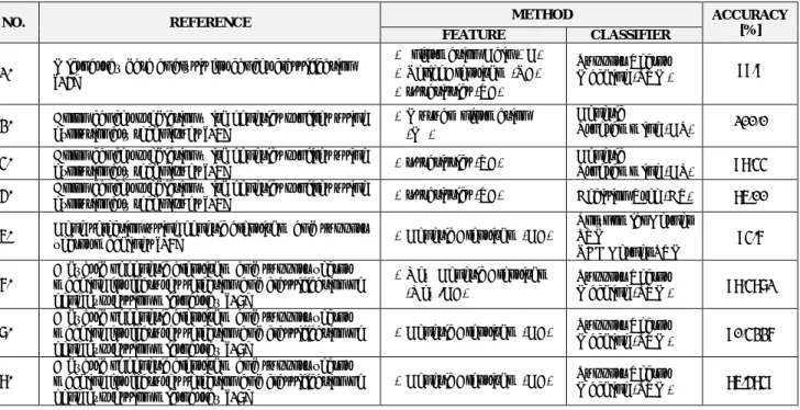
Table 1 presents a summary of findings of recent studies on colon cancer classification accuracy:
Table 1: Literature review on colon cancer classification accuracy
NO. REFERENCE METHOD ACCURACY
[%]
FEATURE CLASSIFIER
1. Microarray data analysis for cancer classification [14]
•Information Gain (IG) •Relief Algorithm (RA) •t-statistics (TA)
Support Vector
Machine (SVM) 99.9
2. Colon cancer prediction with genetics profiles using evolutionary techniques [15]
•Mutual Information (MI)
Genetic
Programming (GP) 100.0
3. Colon cancer prediction with genetics profiles using
evolutionary techniques [15] •t-statistics (TA) Genetic Programming (GP) 98.33
4. Colon cancer prediction with genetics profiles using
evolutionary techniques [15] •t-statistics (TA) Decision Tree (DT) 85.00
5. Gene selection using genetic algorithm and support
vector machines [16] •Genetic Algorithm (GA)
Polynomial Kernel SVM
RBF Kernel SVM 93.6
6. A hybrid of genetic algorithm and support vector machine for features selection and classification of gene expression microarray [17]
•New Genetic Algorithm
(New-GA) Support Vector Machine (SVM) 98.3871 7. A hybrid of genetic algorithm and support vector machine for features selection and classification of
gene expression microarray [17] •
Genetic Algorithm (GA) Support Vector
Machine (SVM) 90.3226
8. A hybrid of genetic algorithm and support vector machine for features selection and classification of
gene expression microarray [17] •
Genetic Algorithm (GA) Support Vector
9. Ensemble machine learning on gene expression
data for cancer classification [18] --- Single C4.5 (DT) 95.16
10. Machine learning in DNA Microarray analysis for cancer classification [19]
•Information Gain (IG) •Mutual Information (MI)
Linear Kernel SVM
RBF Kernel SVM
71.0
11. Machine learning in DNA Microarray analysis for
cancer classification [19] •Euclidean Distance (ED)
Cosine Kernel KNN
Pearson Kernel KNN
93.9
12. Particle swarm optimization for gene selection in classifying cancer classes [20]
•Improved Particle Swarm Optimization (IPSO)
--- 94.19
13. Particle swarm optimization for gene selection in classifying cancer classes [20]
•Binary Particle Swarm
Optimization (BPSO) --- 86.94
14. Applying Data Mining Techniques for Cancer
Classification from Gene Expression Data [21] •t-GA Decision Tree (DT) 89.24
15. Applying Data Mining Techniques for Cancer
Classification from Gene Expression Data [21] •Genetic Algorithm (GA) Decision Tree (DT) 88.80 16. Applying Data Mining Techniques for Cancer
Classification from Gene Expression Data [21] •t-statistics (TA) Decision Tree (DT) 77.42 17. Applying Data Mining Techniques for Cancer
Classification from Gene Expression Data [21] •Information Gain (IG) Decision Tree (DT) 77.26 18. Applying Data Mining Techniques for Cancer
Classification from Gene Expression Data [21] •GS Method Decision Tree (DT) 69.35
19. Integrating Biological Information for Feature Selection in Microarray Data Classification [22]
•Information Gain with
Association Analysis Support Vector Machine (SVM) 93.55 20. Integrating Biological Information for Feature
Selection in Microarray Data Classification [22] •Information Gain (IG)
Support Vector
Machine (SVM) 90.33
21. Colon cancer prediction with genetic profiles using
intelligent techniques [23] •t-statistic (TA) RBF Kernel SVM 84.085
22. Hybrid Methods to Select Informative Gene Sets in
Microarray Data Classification [24] •Genetic Algorithm (GA) Neural Network (NN) 94.92 23. Hybrid Methods to Select Informative Gene Sets in
Microarray Data Classification [24] •Genetic Algorithm (GA) Decision Tree (DT) 96.79 24. Classification of human cancer diseases by gene
expression profiles [56]
•Information Gain & Standard Genetic Algorithm
Genetic
Programming 85.48
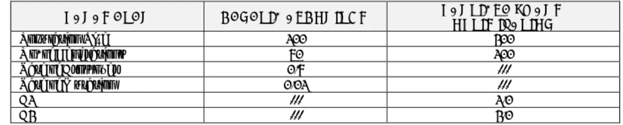
Table 1 shows that 13 out of the 24 methods achieved 90% or above of classification accuracy when applied to the colon cancer dataset, while the remaining achieved classification accuracy of between 69% and 89%. The common algorithms that showed high contribution accuracy in terms of classifications are SVM, GP, and DT. It should be noted that SVM and Genetic Programming have high accuracy results as classifiers when combined with Information Gain and Genetic Algorithms (90% - 100%). The combination of GA and SVM has an accuracy of 85%. GA Method combined with Decision Tree gave the least accurate result: 69%. The table, also presents a finding of different accuracy results with use of the same classification algorithm, i.e. GA+SVM (90% and 85%) and IG+SVM (99.9% and 90%).
2.2. Time Analysis Comparison
Time analysis is considered as part of the computational complexity principle that describes how an algorithm uses resources computationally. The complexity of any algorithm is computed using the Big O notation, which is the expression in the growth rate of a function that describes its higher bound, and is described by the following scheme [47]:
“O(g(n)) = {f |∃ c > 0, ∃ n0, > 0, ∀ n ≥ n0: 0 ≤ f ≤ cg(n)}” (1)
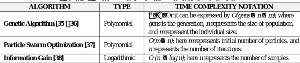
While, “f ∈(g(n)) if, and only if, there exists positive constant c and n0, such that for all n ≥ n0” [34]. Note that the time calculated is the one which was used to build up the process model in the Weka tool. Table 2 illustrates the time complexity (Big O) for most of the feature selection algorithms discussed, while Table 3 presents the same for the classification algorithms:
Table 2: Time complexity in feature selection algorithms
ALGORITHM TYPE TIME COMPLEXITY NOTATION
Genetic Algorithm [35 – 36] Polynomial
𝑂(𝑛2) Or it can be expressed by O(gens × n × m); where gens is the generation, n represents the size of population, and m represent the individual size.
Particle Swarm Optimization [37] Polynomial O(m × n); here m represents initial number of particles, and n represents the number of iterations.
Information Gain [38] Logarithmic O (n × log n); here n represents the number of samples.
Table 3: Feature classification algorithms time complexity
ALGORITHM TYPE TIME COMPLEXITY NOTATION
Support Vector Machine [39 – 40] Polynomial
(Cubic)
𝑂(𝑛3); here n represents the training points number for a classical SVM.
Naïve Bayes [41] Polynomial O(m × n); here m represents number of samples, and n represents the number of features.
Decision Tree [42 – 43] Polynomial 𝑂(𝑚 × 𝑛
2); here m represents the number of training data and n represents the Number of attributes.
Genetic Programming [49 – 50] Logarithmic O (n × log n); here n represents the Number of samples.
Weka is used widely within other research in the area of the study [58]: http://www.cs.waikato.ac.nz/~ml/weka/
The two common methods used in Weka for evaluating data are leave-one-out cross validation (LOOCV) and k-fold cross validation. These methods are used when a real dataset is not available. The contents of the dataset are randomly apportioned into training and testing sets, and different predictors are then compared. LOOCV is a method applied on (n-1) testers and then verified on the remaining ones [9]. The method is reiterated n times in which each sample is left out once at the end [9]. In the k-fold cross validation method, data is arbitrarily allocated to 10 non-overlapping groups (default division of folds) of approximately equal size [48].
2.3. Summary of the Current State of study and limitations
There are noteworthy discrepancies between the proposed approach and the previous studies on colon cancer selection and classification algorithms, as well as on accuracy detection. The following points are discussed about the limitations on the exiting work reflecting the advantage of current studies:
• Table 1 shows 24 different feature selection algorithms as well as classification algorithms,13 algorithms showed 90% or above accuracy using different tools.
• Using the same algorithms and same datasets leads to different accuracy results, as shown by Yeh et al. [21] and Yang and Zhang [24].
• Most of state of the art work explored that SVM gives very competitive results as a classifier algorithm, while PSO shows very good results as a selection algorithm.
•
For example, to the best of the authors’ knowledge, no studies were reported in the literature thatanalyzed the direct relationship between the accuracy of the algorithms implemented and the performance of the time taken to select and classify the features.
• This paper evaluates the performance of the most popular feature selection and classification algorithms implemented for the colon cancer dataset. The paper will determine that algorithms demonstrated the highest accuracy in the colon cancer feature selection and classification process, and finally shows which one quickly corresponds to high accurate classification.
• In this work, the hybridization that has more than one feature selection using the same dataset shows very good results.
Our proposed system, detects the relationship between the algorithm accuracy and the time it requires to detect the colon cancer tumors. This system links the efficiency of algorithms’ performance to the accuracy of the algorithms that have been presented in literature so far.
3. DNA MICROARRAY DATASET AND TECHNIQUES
This section presents an account of how the numeric dataset is generated for the experiments, and defines the feature selection and classification algorithms.
3.1. Background of Datasets
A classic microarray is composed of a large amount of DNA particles spotted in order over a solid material [19]. This technique can examine the gene information in a less time [19].
Currently it is difficult to obtain a central database for human genome data [25]. However, there are plenty of public available gene expression datasets commonly used by researchers in the field of cancer selection and classification experiments. Lists of the most publicly available colon cancer datasets can be found in [6, 8, 26, 27, 28].
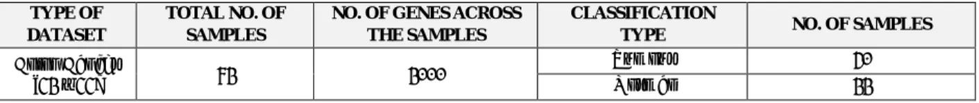
Alon et al. established that the colon cancer dataset is a collection of different expressions that consists of 62 samples (collected from 62 patients) [32] as showing Table 4. It is noteworthy that the “tumour” tissues were obtained from tumours parts of the colon, while the “normal” tissues were derived from healthy tissues of the same colons. According to Archetti et al., approximately 6500 human genes are represented, 2000 of which were extracted and collected. They have shown the better contributions to the expression levels measured [37].
Table 4: Gene expression dataset used in the study TYPE OF
DATASET
TOTAL NO. OF SAMPLES
NO. OF GENES ACROSS THE SAMPLES
CLASSIFICATION
TYPE NO. OF SAMPLES
Colon Cancer
[32 – 33] 62 2000
Tumour 40
Normal 22
3.2. Feature Selection and Classification Techniques
Feature selection over DNA microarray focuses on filter methods [8]. It should be noted that not all the genes measured are required for further analysis because some of them they are uninformative (i.e. not
related) to the classification of cancer; this may affect the operation of some machine learning algorithms [30].
A set of algorithms that have previously demonstrated effectiveness in solving classification problems applied in machine learning studies has been adopted for the current study [19]. Chitode and Nogari defined classification as the process of discovering a prototype that designates and discriminates among different data classes (types) [8]. Classification accuracy is measured in terms of the proportion of expected samples to the overall number of samples, as represented in Equation 1 below [31]:
𝐴𝑐𝑐𝑢𝑟𝑎𝑐𝑦 = 𝑇𝑜𝑡𝑎𝑙 𝑛𝑢𝑚𝑏𝑒𝑟 𝑜𝑓 𝑝𝑟𝑒𝑑𝑖𝑐𝑡𝑒𝑑 𝑠𝑎𝑚𝑝𝑙𝑒𝑠
𝑇𝑜𝑡𝑎𝑙 𝑛𝑢𝑚𝑏𝑒𝑟 𝑜𝑓 𝑠𝑎𝑚𝑝𝑙𝑒𝑠 (2)
Most of the cancer classification models proposed is derived from the statistical and machine learning studies [25]. Based on their survey of previous studies, Ying and Jiawi contend that “there is no single classifier that is superior to the rest” [25]. It is noteworthy from these studies of proposed algorithms that most studies were interested only with classification accuracy in the analysis of the data without paying much attention to the algorithm running time. In summary, it is found that:
• DNA microarray technology offers a method of numerically analyzing the data, but needs normalization for experiment conducting.
• The searching algorithms undertake the process of identification of informative genes.
• The classification algorithms undertake the process of classifying the feature data into cancer or normal. 4. METHODOLOGY
This section will discuss the methodology of the work that was carried out, including the flowchart, data sources, and instrumentation. The approach has three component parts: (1) study and analysis of the performance of the feature selection algorithms as applied to the colon dataset; (2) analysis of the performance of the classification algorithms across the same dataset and (3) analysis of the performance of the combination of both selection and classification algorithms.
4.1. Proposed System
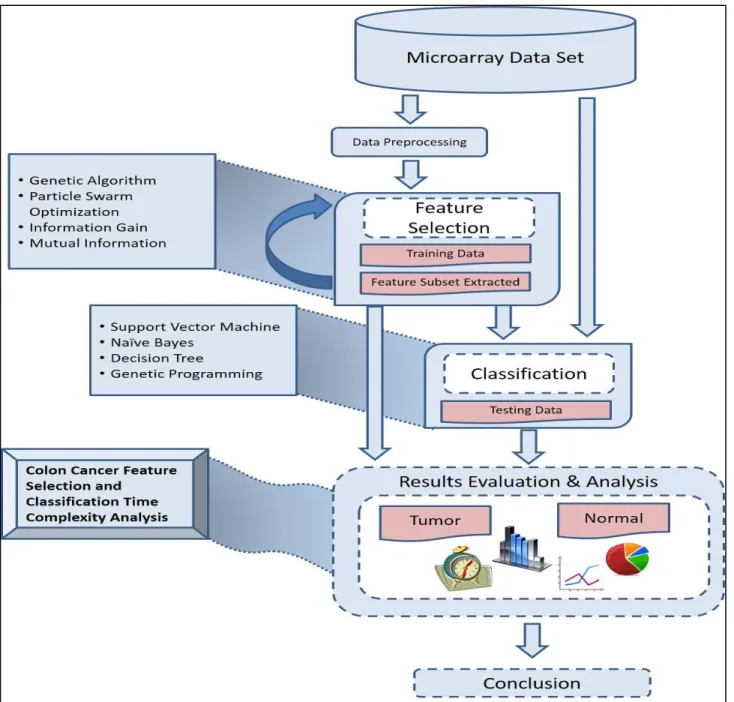
The flow chart shown in Figure 1 illustrates how the experimental system was planned to operate in terms of applying feature selection and classification algorithms within the three phases discussed earlier. 4.2. Data sources and tools
The data used in the study were extracted from one of the public cancer datasets [32] that have been extensively used by researchers in the field; these were available free of charge online, as discussed in Section 3.1. The computational tool used for all the experiments described was the Weka Machine Learning package and its associated libraries; see Section 2.2 above. The computing environment for the experiments used a PC with the Windows 8.1 operating system, a 1.8 GHz Intel Core i5 processor and 8 GB of installed RAM.
Fig. 1: Proposed system flowchart/ workflow
5. EXPERIMENTAL PREPARATION
In this section, the experimental preparation is described as follows: (1) Definition of experiment methods; (2) Data preparation; and (3) The experimental Setup.
5.1. Definition of experimental methods
As the number of samples used in the experiments was small, cross validation was adopted as the measure of performance. The procedure was repeated 10 times to make each set acts as a test set; see Sections 2.2 and 3.1 for related background information.
5.2. Data Preparation
One of the challenges posed by genetic data analysis is the small number of samples compared to the associated large number of genes. One way of addressing this situation is to use feature reduction, which transforms the raw data into a form that is suitable for analysis. A normalization procedure may be used for this, where classification algorithms are able to use the gene expression measurements just as they are. Once the data have been prepared, the next step is the feature selection process that reduces the dimensionality of the dataset. Thus, before using the colon dataset in our work, we normalized the data using the min-max normalization procedure by applying the following formula:
x[i] = (x[𝑖] − minValue)
(maxValue − minValue) (3)
Where x is the attribute, i represents the amount of the samples, minValue represents the lowest value of each attribute, and maxValue represents the highest value of each attribute.
5.3. Experimental setup
The parameter settings for the Genetic Algorithm and the Particle Swarm Optimization algorithms are presented in Table 5. For each algorithm, these parameter values were changed one by one until adopt the objective values based on the solution quality and high performance results. Default parameters were used for the remainder of the algorithms, as they had demonstrated good results in the experiments. Appendix A, presents the default parameters and also describes some several random test evaluations that were conducted to select the anticipated parameters; which account for and reflects the reasoning behind the selection of the parameters.
Table 5: Gene expression dataset used in the study
PARAMETER GENETIC ALGORITHM PARTICLE SWARM OPTIMIZATION
Population Size 100 200 No. of Generations 50 100 Rate of Crossover 0.6 --- Rate of Mutation 0.01 --- C1 --- 1.0 C2 --- 2.0 6. RESULTS
The experiments took place in multiple phases. Phase One was to implement the feature selection algorithms (GA, PSO, and IG) across the dataset; Phase Two was to implement the classification algorithms only using the original dataset without prior application of any feature selection algorithms; Phase Three was to implement the hybridization and combining techniques of the feature selection and classification algorithms together. More details of the analysis of these phases, and the discussion of results, are presented in the following sections.
6.1. On Phase One
The experiment in this phase studied the difference between the selection algorithms GA, PSO and IG in relation to the number of genes selected from the normalized benchmark colon dataset described above in association with the list of parameters given in Table 5 and in Appendix A.
There are two main classical methods for feature selection: the first one is the filter method, which makes an independent assessment over the dataset attributes; the second one is the wrapper method, which applies an evaluation of learning algorithm; thus the learning algorithm will be wrapped into the selection technique [44].
Feature selection identifies the relevant genes within the colon cancer dataset. This step is used to select the best attributes of the dataset. Using the Weka data-mining tool, feature selection can be applied using three methods, as presented in Table 6.
Table 6: Attribute evaluation methods for attribute selections
ATTRIBUTE SUBSET EVALUATOR
METHOD
NAME FUNCTION
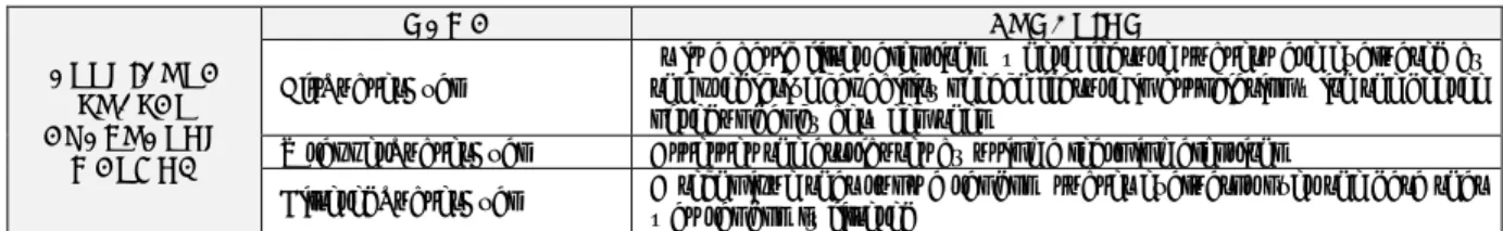
CfsSubsetEval It is a basic filter algorithm where feature subsets are evaluated by the predictive capability of each feature in association with the degree of redundancy between them
WrapperSubsetEval Assesses the attributes by using a learning algorithm
FilteredSubsetEval A technique that runs a random subset evaluator over the data that was randomly filtered
Table 7 presents the number of selected features (genes) using the GA and the PSO algorithms by applying different attribute evaluation methods for attribute selections.
Table 7: Number of features retrieved by applying GA and PSO as feature selection algorithms on the colon dataset
FEATURE SELECTION USING CFSSUBSETEVAL METHOD
GA 412
PSO 29
FEATURE SELECTION USING WRAPPERSUBSETEVAL METHOD
GA + SVM 958
GA + Naïve Bayes 817
GA + DT 465
PSO + SVM 112
PSO + Naïve Bayes 122
PSO + DT 543
FEATURE SELECTION USING FILTEREDSUBSETEVAL METHOD
GA + SVM 205
GA + Naïve Bayes 482
GA + DT 62
PSO + SVM 104
PSO + Naïve Bayes 175
PSO + DT 38
From Table 7, it is apparent that in general the PSO algorithm had reduced the number of selected genes much better compared with GA. When applied using the CfsSubsetEval Method, PSO had selected 29 genes, which is almost 14 times less than GA using the same method. Also, when applied using the WrapperSubsetEval method along with SVM, 112 genes were selected, compared with the GA when wrapped with the same algorithm (SVM) or with other classification algorithms using the same method. In addition, when it was applied using the FilteredSubsetEval method, it showed good results also with the
DT algorithm (38 genes selected) in comparison with the GA using the same method as well. However, the classifier approach applied with GA using Decision Tree (DT), gave good results (62 genes selected). Note that the IG (Information Gain) and the MI (Mutual Information) are used as ranking methods for feature selection. A threshold value is required for these algorithms, so a value of 0 was selected as a threshold; if the weight of features is greater than 0 they will be selected, otherwise they will be discarded. In our experiments is showed high contribution (134 genes selected). Thus, genes with discriminative values equal to zero were discarded.
Another proposed combination algorithm was constructed by combining feature selection algorithms. First, it applied GA followed by PSO as a hybrid combined feature selection procedure. Thus, GA was applied initially to the original benchmark colon dataset to select a feature subset, and then the PSO was applied later over the newly selected subset. We reversed the algorithms and applied initially the PSO, then subsequently the GA as a hybrid feature selector, as previously. Table 8 and Table 9 respectively present the results, and reflect how GA/PSO using classifier subset evaluation can select subsets with fewer features. The proposed combined algorithms show highly selective and accurate results.
Table 8: Applying GA/PSO as a hybrid features model using the efficiency of the different selection methods
METHOD NO. OF FEATURES SELECTED BY GA/PSO
Using CFS 22
Using Wrapper (DT) 24
Using Classifier (Naïve Bayes) 4
Table 9: Applying PSO/GA as a hybrid feature selection model using the efficiency of the different selection methods
METHOD NO. OF FEATURES SELECTED BY PSO/GA
Using CFS 12
Using Wrapper (DT) 10
Using Classifier (Naïve Bayes) 13
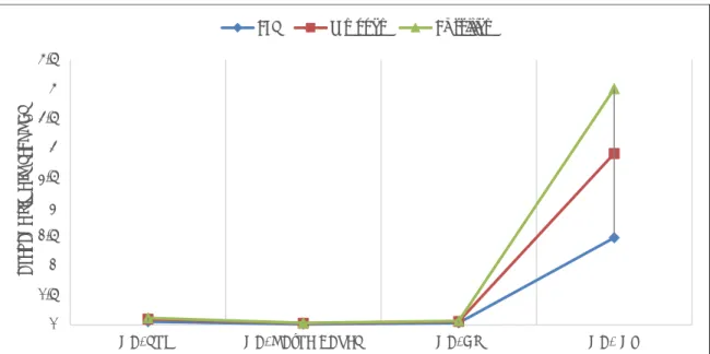
Figure 2 summarizes the feature selection difference between all the methods applied so far. It is noticeable that GA selects more data (more than 400 genes) in comparison to PSO, which selects fewer (29 – 100 genes). It is found that the combination of GA and PSO together results in fewer genes being selected (4 genes).
Fig. 2: Feature subset selections using feature algorithms
6.2. On Phase Two
In this phase, classification algorithms (SVM, Naïve Bayes, Decision Tree, and Genetic Programming) were implemented using the default parameters in Weka, without the contribution of any feature selection algorithm, thus only machine learning algorithms were implemented. The experiments were conducted with the first 10, 50, 100, 500, 1000, 1500, and 2000 (the whole colon dataset) attributes using cross validation and applying the default parameters (see Appendix A).
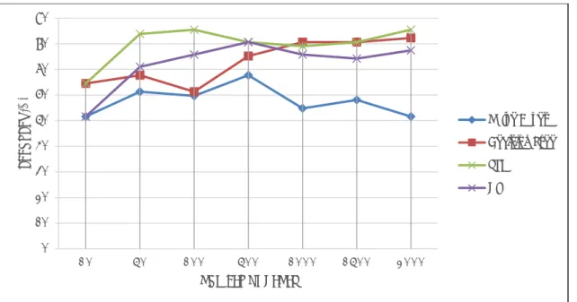
Figure 3 presents the records obtained for accuracy of classification compared to the number of genes as an input. It may be observed that SVM results in better accuracy over other classification algorithms (86%) when applied to the full dataset, while Naïve Bayes has the lowest accuracy (52%).
0 50 100 150 200 250 300 350 400 450 500 N u mb e r o f F e atu re s ( Ge n e s) S e le cte d
Fig. 3: Classification accuracy for different gene samples
Figure 4 shows the time taken to classify the various gene samples. It can be seen that for a smaller number of genes, almost all the classification algorithms require less time (processing is almost instantaneous), but for a large number of genes it is observed that the Genetic Programming takes more time (up to 6 seconds). That is, when the amount of input increases, the function of Genetic Programming has a big O(𝑛𝑙𝑜𝑔𝑛). So, SVM is considered to be an accurate and fast classification algorithm compared to others.
Fig. 4: Classification time for different gene samples
0 10 20 30 40 50 60 70 80 90 1 0 5 0 1 0 0 5 0 0 1 0 0 0 1 5 0 0 2 0 0 0 A CCURA CY ( % ) NUMBER OF GENES Naïve Bayes Decision Tree SVM GP 0 1 2 3 4 5 6 7 10 50 100 500 1000 1500 2000 Tim e in Se con d s Number of Genes Naïve Bayse Decision Tree SVM GP
6.3. On Phase Three:
The procedure in this phase is to apply the classification algorithms after applying efficient selection algorithms, i.e. those which were implemented in Phase One earlier (section 6.1). Default parameters for classification algorithms were applied (see Appendix A), and the same experimental conditions and tools were used as for Phases One and Two (sections 6.1 and 6.2). The experiments were conducted by using a number of respectively selected features (genes) from the reduced colon dataset attributes. The detailed data are presented in Appendix B.
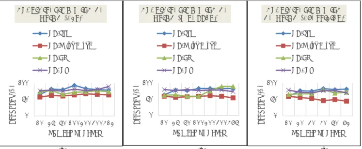
(a) (b) (c) Fig. 5: Accuracy of classification for hybridization with GA using multiple feature selection techniques
As shown in Figure 5, it is found that both GA/SVM using the three attribute evaluation techniques in (a), (b), and (c) perform more accurately than others, above 80% accuracy; the analysis of time complexity for GA/SVM is O (𝑛3+ 𝑛2), as the SVM has a polynomial (cubic) time complexity notation, which is higher than
others. However, the GA/DT and GA/GP outperform other algorithms in terms of classification accuracy; they achieve to 90% accuracy. It is apparent that GA/Naïve Bayes is the least accurate.
Figure 6 shows that GA/Naïve Bayes takes less time to classify different genes if applied with all selection techniques (almost instantaneous), but results in reduced accuracy, as indicated, while GA/GP is more accurate but also takes longer (up to 4 seconds) than other algorithms.
0 50 100 1 0 2 5 5 0 1 0 0 2 0 0 3 0 0 4 1 2 A CCURA CY ( % ) NUMBER OF GENES H Y B R I D I S A T I O N W I T H G A U S I N G ( C F S ) GA/SVM GA/Naïve Bayes GA/DT GA/ GP 0 50 100 1 0 2 5 5 0 1 0 0 2 0 0 3 0 0 4 6 5 A CCURA CY ( % ) NUMBER OF GENES H Y B R I D I S A T I O N W I T H G A U S I N G ( W R A P P E R ) GA/SVM GA/Naïve Bayes GA/DT GA/ GP 0 50 100 1 0 2 0 3 0 4 0 5 0 6 2 A CCURA CY ( % ) NUMBER OF GENES H Y B R I D I S A T I O N W I T H G A U S I N G ( C L A S S I F I E R ) GA/SVM GA/Naïve Bayes GA/DT GA / GP
Fig. 6: Classification time for different gene samples using the hybridization with GA
However, it is apparent from figure 7 (a, b, & c) that PSO/SVM achieves better average classification accuracy by applying the CFS (87%) and wrapper methods (87%); the time complexity of PSO/SVM is
O(𝑀𝑁 + 𝑛3), while PSO/DT performs better using the classifier method; the time complexity of PSO/DT is
O(𝑀𝑁 + 𝑚𝑛2).
(a) (b) (c)
Fig. 7: Accuracy of classification for hybridization with PSO using different feature selection techniques Figure 8 shows that PSO/SVM and PSO/DT take less average time (almost instantaneous) to classify different genes. That is, they showed high classification accuracy with minimal time, whereas PSO/GP takes longer (up to 3 seconds).
0 0.5 1 1.5 2 2.5 3 3.5 4 4.5 G A / S V M G A / N A Ï V E B A Y E S G A / D T G A / G P A V ER A G E T IME IN S ECO N DS CFS Wrapper Classifier 0 100 5 1 0 1 5 2 9 A CCURA CY ( % ) NUMBER OF GENES A C C U R A C Y O F C L A S S I F I C A T I O N F O R H Y B R I D I S A T I O N W I T H P S O U S I N G ( C F S ) PSO/SVM PSO/Naïve Bayes PSO/DT PSO/ GP 0 50 100 1 0 2 5 5 0 7 5 1 0 0 1 1 2 A CCURA CY ( % ) NUMBER OF GENES A C C U R A C Y O F C L A S S I F I C A T I O N F O R H Y B R I D I S A T I O N W I T H P S O U S I N G ( W R A P P E R ) PSO/SVM PSO/Naïve Bayes PSO/DT 0 50 100 5 1 0 1 5 2 0 2 5 3 0 3 8 A CCURA CY ( % ) NUMBER OF GENES A C C U R A C Y O F C L A S S I F I C A T I O N F O R H Y B R I D I S A T I O N W I T H G A U S I N G ( C L A S S I F I E R ) PSO/SVM PSO/Naïve Bayes PSO/DT PSO/ GP
Fig. 8: Classification time for different gene samples using the hybridization with PSO
Fig. 9: Accuracy of classification for hybridization with IG
From Figure 9, it is clear that IG/DT (86%), and IG/SVM (86%) perform more accurately on average than others; the time complexity of IG/DT is O(𝑛𝑙𝑜𝑔𝑛 + 𝑚𝑛2), and for IG/SVM is O(𝑛𝑙𝑜𝑔𝑛 + 𝑚𝑛3). Overall, IG/DT
outperforms all other algorithms in relation to classification accuracy with the full dataset (134 genes, around 88.7%), but IG/SVM still generates similar results for accuracy. IG/Naïve Bayes performs less well than the other algorithms (81%).
0 0.5 1 1.5 2 2.5 3 3.5
PSO/SVM PSO/Naïve Bayes PSO/DT PSO/GP
A ve rag e Ti me in S ec o n d s CFS Wrapper Classifier 70 72 74 76 78 80 82 84 86 88 90 1 0 2 5 5 0 7 5 1 0 0 1 1 0 1 2 5 1 3 4 A CCURA CY ( % ) NUMBER OF GENES IG/SVM IG/Naïve Bayes IG/ DT IG/GP
Figure 10 shows that, with a small number of genes (fewer than the first 100), IG/Naïve Bayes and IG/DT are almost instantaneous, but with the full dataset selected, IG/GP takes longer (almost 1.5 seconds).
Fig.10: Classification time for different gene samples using the hybridization with IG 7. DISCUSSION AND ANALYSIS
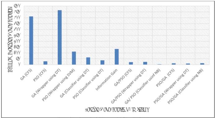
Based on the above results, it is found that the PSO as a selection algorithm outperforms the others. However, IG is efficient in ranking the genes and hence in selecting the best-ranked ones thereafter. From the previous experiments and as presented in Figure 11, the PSO/SVM method demonstrated the highest average accuracy (87%) in terms of classifying colon cancer datasets compared with the other algorithms presented earlier. IG/SVM (86%) and IG/DT (86%) demonstrate very good classification accuracy. PSO/DT has less classification accuracy (71%).
Fig. 11: Hybrid classification algorithms average accuracy
0 0.2 0.4 0.6 0.8 1 1.2 1.4 1.6 1.8 1 0 2 5 5 0 7 5 1 0 0 1 1 0 1 2 5 1 3 4 TIME IN S ECO N DS NUMBER OF GENES IG/SVM IG/Naïve Bayes IG/ DT IG/GP 0 10 20 30 40 50 60 70 80 90 GA/SVM (CFS) GA/SVM (Wrapper) GA/SVM (Classifier) PSO/SVM (CFS) PSO/SVM (Wrapper) PSO/DT (Classifier) IG/SVM IG/DT
Finally, Table 10 concludes all the average accuracies resulted from the previous experiments when applied to full data set. There were found to be 12 algorithmic methods that have accuracy above 80% when applied to the full dataset; three algorithms have accuracy of 90% or more. One algorithm scored below 50%.
Table 10: Hybrid average accuracy applied on selected feature subsets and on full selected datasets
SELECTION
METHOD ALGORITHMS
AVERAGE ACCURACY [%]
FULL DATA SET ACCURACY [%] CFS
GA/ SVM 81 79
GA/ Naïve Bayes 64 65
GA / DT 74 74
GA/ GP 80 90
Wrapper
GA/ SVM 80 84
GA/ Naïve Bayes 59 59
GA / DT 72 90
GA/ GP 78 74
Classifier
GA/ SVM 77 82
GA/ Naïve Bayes 52 45
GA / DT 71 73
GA/ GP 75 71
CFS
PSO/ SVM 87 89
PSO/ Naïve Bayes 75 82
PSO/ DT 82 79
PSO/ GP 84 81
Wrapper
PSO/ SVM 87 94
PSO/ Naïve Bayes 61 58
PSO/ DT 72 71
PSO/ GP 77 84
Classifier
PSO/ SVM 66 66
PSO/ Naïve Bayes 55 55
PSO/ DT 71 71
PSO/ GP 64 68
Information Gain Ranker
IG/ SVM 86 84
IG/ Naïve Bayes 81 79
IG / DT 86 89
IG/ GP 85 84
Many approaches in the literature had touched the colon cancer classification accuracy as presented in Table 1 section 2.1, which achieved 93.6% as with Shatoa et al. [16], and Cho et al. [19], while Huey et al. [22] achieved 93.5%, others like Yeh et al. achieved 89.2% [21], Salem et al. achieved 85.48% [56], and other contributions achieved 84% as with Alladi et al. in [23]. This investigation using PSO/SVM achieved a better outcome, i.e. 94%. That is, better classification accuracy when applied to all selected features using the wrapper selection method based on the parameters and experimental conditions applied and by using the same colon cancer dataset.
On the other hand, in this investigation using GA/DT and GA/GP had 90% classification accuracy that outperforms the results of Yeh et al. (89%) [21] and Salem et al (85%) [56] respectively. Also, by using IG/DT the classification accuracy had 89%when applied to the whole dataset, which outperforms the results (77%) in [21] using almost same experiment conditions as well as the same dataset.
To our knowledge, the classification of colon cancer studies presented in Table 1 earlier, didn’t report the efficiency of algorithms in terms of time performance analysis except in the study of Salem et al [56] where the complexity time is almost equivalent to O(𝑛2 (n log n + 𝑛2)). In their work, they implemented the model
of using the selection algorithm first (IG), followed by a reduction algorithm (sGA), and at the end applied the classification algorithm (GP). In this paper, we studied the algorithms related in three distinct phases and found that applying feature selection algorithm, followed by a classification algorithm only (PSO/ SVM) improved the classification accuracy 94% and resulted in a more efficient time O(𝑀𝑁 + 𝑛3) when compared
with the results of others in the literature (especially when compared with the time analysis work of [56] in terms of time analysis using the same dataset and the selection of population size but with some minor difference in the parameters rate for the GA algorithm, as indicated in Appendix A).
We found that our work takes almost an instantaneous time in seconds to classify genes (almost 0 seconds) while the other work such as in [56] takes more extensive time to do the same job. For that, our algorithm is considered computationally less expensive when compared with others.
8. CONCLUSIONS AND FUTURE WORK
In conclusion, the paper has achieved its objective by studying the enactment of the common feature selection and classification algorithms for the colon cancer dataset, but the new motivation was to compare the accuracy of and analyze the time complexity for these algorithms to determine which algorithm provides the most accurate output in correlation with time complexity analysis. The study was implemented over a colon cancer dataset of 2000 genes, by applying three typical and main feature selection algorithms: Genetic Algorithm, Particle Swarm Optimization, and Information Gain, and using four common classification algorithms: Support Vector Machine, Naïve Bayes, Decision Tree, and Genetic Programming. A three-phase experimental design was followed:
• Phase One studied the difference among multiple selection algorithms, and found that the PSO algorithm outperforms the GA algorithm when applied directly to select subset features that reduce the population size for the classification algorithm either using the CFS, the wrapper approach or the classifier approach.
• In Phase Two, classification algorithms were implemented alone without the contribution of any selection algorithm; it was found that SVM has better classification accuracy with a big O
(𝑛
3)
.• In Phase Three, a comparison between applying a hybrid combination of selection and classification algorithms was undertaken. The best algorithm that expressed the high performance with a big growth rate of time complexity was the hybridization of the PSO combined with the SVM (average 87%) but when applied to all the feature subset selection it achieved an accuracy up to 94%.
The results of the experiments figured that applying feature selection algorithms prior to classification algorithms results in better accuracy than when the latter are applied alone. Without feature selection, use of SVM as a classifier yielded (85%) accuracy, compared with when implemented with a feature selection algorithm first: PSO/SVM (94%). Moreover, comparing between filter and wrapper selection methods when applied to the full microarray dataset, the wrapper methods yield more accurate results than the filter models. As a result, PSO/SVM can be considered a suitable algorithm for colon cancer selection and classification in medical research. Moreover, the SVM showed a polynomial (cubic) growth rate, while GA, IG, and PSO showed a quadratic polynomial growth rate. The other classification algorithms showed a quadratic polynomial growth rate. For that, SVM has the highest Big O magnitude of time complexity. For the future work, more efforts will be made to access other medical records for the colon cancer as well as to use other machine learning tools and compare the results with Weka. Moreover, the study can be extended to the applications of the selection and classification algorithms that have demonstrated the practical values in studying an expanded range of cancer datasets other than the colon cancer only.
REFERENCES
[1] S. Shah and A. Kusaik, (February 2007) "Cancer gene search with data-mining and genetic algorithms," Computers in Biology and Medicine, vol. 37, no. 2, pp. 251-261. DOI: http://dx.doi.org/10.1016/j.compbiomed.2006.01.007
[2] B. W. Stewart and C. P. Wild, (2014) "World Cancer Report," International Agency for Research on Cancer, Lyon, France. [3] M. Mohamad, S. Omatu, M. Yoshioka and S. Deris, (2008)"An Approach Using Hybrid Methods to Select Informative Genes from Microarray Data for Cancer Classification," in Second Asia International Conference on Modeling & Simulation, AICMS 08.
[4] N. Revathy and R. Almalraj, (January 2011) "Accurate Cancer Classification using Expressions of Very Few Genes," International Journal of Computer Applications, vol. 14, no. 4, p. 0975 – 8887. DOI: http://dx.doi.org/10.5120/1832-2452
[5] S. Mukkamala, Q. Liu, R. Veeraghattam and A. Sung, (2005) "Computational Intelligent Techniques for tumor classification using microarray gene expression data," International Journal of Lateral Computing, vol. 2, no. 1, pp. 38-45.
[6] E. Venkatesh, P. Tangaraj and S. Chitra, (Feb. 2010) "Classification of cancer gene expressions from micro-array analysis," in International Conference on Innovative Computing Technologies (ICICT), 2010, pp. 12-13. DOI: http://dx.doi.org/10.1109/ICINNOVCT.2010.5440095
[7] V. P. Khobragade and D. Vinayababu, (2012) "A Comparative Analysis of Hybrid Approach for Gene Cancer Classification using Genetic Algorithm and FFBNN with Classifiers ANFIS and Fuzzy NN," IOSR Journal of Engineering, vol. 2, no. 11. DOI: http://dx.doi.org/10.9790/3021-021134452
[8] K. Chitode and M. Nagori, (November 2013) "A Comparative Study of Microarray Data Analysis for Cancer Classification," International Journal of Computer Applications, vol. 81, no. 15, p. 0975 – 8887. DOI: http://dx.doi.org/10.5120/14198-2392
[9] J. Jäger, R. Sengupta, & W.L. Ruzzo, (Dec. 2002). “Improved gene selection for classification of microarrays”. In Proceedings of the eighth Pacific Symposium on Biocomputing: 3–7 January 2003; Lihue, Hawaii, pp. 53-64.
[10] Y. Saeys, I. Inza and P. Larrañaga, (2007) "A review of feature selection techniques in bioinformatics," Bioinformatics 23, p. 2507– 2517. DOI: http://dx.doi.org/10.1093/bioinformatics/btm344
[11] F. Han, S. Yang, and J. Guan. 2015. An effective hybrid approach of gene selection and classification for microarray data based on clustering and particle swarm optimisation. Int. J. Data Min. Bioinformatics 13, 2 (August 2015), 103-121.
[12] E. Alba, J. Garcia-Nieto, L. Jourdan and E. Talbi, (Sept. 2007) "Gene selection in cancer classification using PSO/SVM and GA/SVM hybrid algorithms" in IEEE Congress on Evolutionary Computation, 2007. CEC 2007. pp.284-290. DOI: http://dx.doi.org/10.1109/CEC.2007.4424483
[13] J. Hua, W. D. Tembe and E. R. Dougherty, (2009) "Performance of feature-selection methods in the classification of high-dimension data," Pattern Recognition, vol. 42, no. 3, pp. 409-424. DOI: http://dx.doi.org/10.1016/j.patcog.2008.08.001
[14] A. Osareh and B. Shadgar, (April 2010) "Microarray data analysis for cancer classification," in 5th International Symposium on Health Informatics and Bioinformatics (HIBIT), 2010, pp.125-132. DOI: http://dx.doi.org/10.1109/HIBIT.2010.5478893
[15] A. Kulkarni, B.S.C. Naveen Kumar, V. Ravi, and U. Murthy, (March 2011) “Colon cancer prediction with genetics profiles using evolutionary techniques”, Expert Systems with Applications, vol. 38, no. 3, pp. 2752-2757, DOI http://dx.doi.org/10.1016/j.eswa.2010.08.065.
[16] L. Shutao, W. Xixian and H. Xiaoyan, (2008) "Gene selection using genetic algorithm and support vector machines," Soft Computing, vol. 12, no. 7, pp. 693-698. DOI:10.1007/s00500-007-0251-
[17] M. Mohamad, S. Deris and R. Illias, (2005) "A hybrid of genetic algorithm and support vector machine for features selection and classification of gene expression microarray," International Journal of Computational Intelligence and Applications, vol. 5, pp. 91-107. DOI: http://dx.doi.org/10.1142/S1469026805001465
[18] AC. Tan, and D. Gilbert, (2003) "Ensemble machine learning on gene expression data for cancer classification," Applied bioinformatics, vol. 2, no. 3, pp: 1-10.
[19] S.-B. Cho and H.-H. Won, (2003) "Machine learning in DNA Microarray analysis for cancer classification," in Proceedings of the First Asia-Pacific Bioinformatics Conference. Australian Computer Society; p. 189- 98, Australia.
[20] M. S. Mohamad, S. Omatu, S. Deris, and M. Yoshioka, (2009) "Particle swarm optimization for gene selection in classifying cancer classes," in Proceedings of the 14th International Symposium on Artificial Life and Robotics; pp. 762–765. DOI: 10.1007/s10015-009-0712-z
[21] J.-Y. Yeh, T.-S. Wu, M.-C. Wu and D.-M. Chang, (2007) "Applying Data Mining Techniques for Cancer Classification from Gene Expression Data," in International Conference on Convergence Information Technology, vol. 703, no. 708, pp. 21-23. DOI: http://dx.doi.org/10.1109/ICCIT.2007.153
[22] F. One Huey, M. Norwati and M. N. Sulaiman, (2010) "Integrating Biological Information for Feature Selection in Microarray Data Classification," in Second International Conference on Computer Engineering and Applications IEEE, pp. 330-334. DOI: http://doi.ieeecomputersociety.org/10.1109/ICCEA.2010.215
[23] S. M. Alladi, S. Shantosh, V. Ravi, and U. S. Murthy, (2008). “Colon cancer prediction with genetic profiles using intelligent techniques”. Bioinformation, vol. 3, no. 3, pp. 130–133. DOI: http://dx.doi.org/10.6026/97320630003130
[24] P. Yang and Z. Zhang, (2007) "Hybrid Methods to Select Informative Gene Sets in Microarray Data Classification," in Proceedings of the 20th Australian Joint Conference on Artificial Intelligence, LNAI 4830, pp. 811-815. DOI: http://dx.doi.org/10.1007/978-3-540-76928-6_97
[25] Y. Lu, and J. Han, (June 2003) “Cancer classification using gene expression data”, Information Systems, vol. 28, no. 4, pp. 243 -268, DOI: http://dx.doi.org/10.1016/S0306-4379(02)00072-8.
[26] L. Jourdan, S. Dhaenens and E.-G. Talbi, (2001) "A genetic algorithm for feature selection in data-mining for genetics", in Proceedings of the 4th Metaheuristics International ConferencePorto (MIC’2001), Porto, Portugal, pp. 29–34
[27] L. Wang, F. Chu, W. Xie, (2007) "Accurate cancer classification using expressions of very few genes," IEEE/ACM Transactions on Computational Biology and Bioinformatics, vol. 4, no. 1, pp. 40-53. DOI: http://dx.doi.org/10.1109/TCBB.2007.1006
[28] D. Rhodes, J. Yu, K. Shanker, N. Deshpande, R. Varambally, D. Ghosh, T. Barrette, A. Pandey and A. Chinnaiyan, (2004) "ONCOMINE: a cancer microarray database and integrated data-mining platform," Neoplasia 2004, vol. 6, pp. 1-6. DOI: http://dx.doi.org/10.1016/S1476-5586(04)80047-2
[29] M. Al-Rajab and J. Lu, (2014) "Algorithms Implemented for Cancer Gene Searching and Classifications," Bioinformatics Research and Applications, Lecture Notes in Computer Science, vol. 8492, pp. 59-70. DOI: http://dx.doi.org/10.1007/978-3-319-08171-7_6 [30] W. Yu, T. Igor V., A. H. Mark, F. Eibe, F. Axel, F. X. M. Klaus and W. M. Hans, (February 2005) "Gene selection from microarray data for cancer classification—a machine learning approach”, Computational Biology and Chemistry, v. 29, no. 1, pp. 37-46, DOI: http://dx.doi.org/10.1016/j.compbiolchem.2004.11.001
[31] Z. Cai, R. Goebel, M. Salavatipour and G. Lin, (2007) "Selecting Dissimilar Genes for Multi-Class Classification, an Application in Cancer Subtyping," BMC Bioinformatics, vol. 8, p. 206, DOI: http://dx.doi.org/10.1186/1471-2105-8-206
[32] U. Alon, N. Barkai, D. Notterman, K. Gish, S. Ybarra, D. Mack and A. Levine, (1999) "Broad patterns of gene expression revealed by clustering analysis of tumor and normal colon tissues probed by oligonucleotide arrays," Proceedings of the National Academy of Sciences, USA, vol. 96, no. 12, pp. 6745-6750. DOI: http://dx.doi.org/10.1073/pnas.96.12.6745
[33] F. Archetti, M. Castelli, I. Giordani and L. Vanneschi, (2008) "Classification of colon tumor tissues using genetic programming," in Proceedings of the Annual Italian Workshop on Artificial Life and Evolutionary Computation, pp. 49-58, DOI: http://dx.doi.org/10.1142/9789814287456_0004
[34] P. E. Black, big-O notation, (2008) “Dictionary of Algorithms and Data Structures [online]@, U.S.: Retrieved from the National Institute of Standards and Technology. https://www.nist.gov/dads/HTML/bigOnotation.html
[35] L. Y. Tseng and S. B. Yang, (2001) “A genetic approach to the automatic clustering problem,” Pattern Recognition, vol. 34, no. 2, pp. 415–424. DOI: http://dx.doi.org/10.1016/S0031-3203(00)00005-4
[36] C.-W. Tsai, S.-P. Tseng, M.-C. Chiang, C.-S. Yang, and T.-P. Hong, (2014) “A High-Performance Genetic Algorithm: Using Traveling Salesman Problem as a Case,” The Scientific World Journal, vol. 2014, Article ID 178621. DOI: http://dx.doi.org/10.1155/2014/178621
[37] T. R. Lakshmana, C. Botella and T. Svensson (2012), “Partial joint processing with efficient backhauling using particle swarm optimization,” EURASIP Journal on Wireless Communications and Networking, vol. 2012, no. 1, p. 182. DOI: http://dx.doi.org/10.1186/1687-1499-2012-182
[38] C.-H. Yang, L.-Y. Chuang, and C.-H. Yang, (2010) “IG-GA: a hybrid filter/wrapper method for feature selection of microarray data,” Journal of Medical and Biological Engineering, vol. 30, no. 1, pp. 23–28.
[39] I. W. Tsang, J. T. Kwok, and P.-M. Cheung. (December 2005) “Core Vector Machines: Fast SVM Training on Very Large Data Sets”. Journal of Machine Learning Research, vol. 6, pp. 363-392.
[40] A. Abdiansah and R. Wardoyo. (October 2015) Article: “Time Complexity Analysis of Support Vector Machines (SVM) in LibSVM”. International Journal of Computer Applications, vol. 128, no. 3, pp. 28-34. DOI: http://dx.doi.org/10.5120/ijca2015906480
[41] G. I. Webb, J. R. Boughton, and Z. Wang, (2005). “Not so naive Bayes: Aggregating one-dependence estimators”. Machine Learning, vol. 58, no. 1, pp. 5–24. DOI: http://dx.doi.org/10.1007/s10994-005-4258-6
[42] J. Su and H. Zhang. (2006) “A fast decision tree learning algorithm”. In Proceedings of the 21st national conference on Artificial intelligence (AAAI'06) – Anthony Cohn (Ed.), vol. 1. pp. 500-505.
[43] M.I. Sumam, M. E. Sudheep, and A. Joseph. (2013) "A Novel Decision Tree Algorithm for Numeric Datasets-C 4.5* Stat.". International Journal of Advanced Computing, ISSN:2051-0845, vol. 36, no.1.
[44] M. S. Mohamad, S. Omatu, S. Deris, M. F. Misman, M. Yoshioka. (2009) "A multi-objective strategy in genetic algorithms for gene selection of gene expression data." Artificial Life and Robotics, vol. 13, no. 2, pp. 410-413. DOI: http://dx.doi.org/10.1007/s10015-008-0533-5
[45] E. Bonilla-Huerta, A. Hernandez-Montiel, R. M. Caporal and M. A. Lopez. (2016) "Hybrid Framework Using Multiple-Filters and an Embedded Approach for an Efficient Selection and Classification of Microarray Data," in IEEE/ACM Transactions on Computational Biology and Bioinformatics, vol. 13, no. 1, pp. 12-26. DOI: http://dx.doi.org/10.1109/TCBB.2015.2474384
[46] Jeyachidra and Punithavalli, 2014. “Distinguishability based weighted feature selection using column wise k neighborhood for the classification of gene microarray dataset”, American Journal of Applied Sciences, vol. 11, no. 1, pp 1-7. DOI: http://dx.doi.org/10.3844/ajassp.2014.1.7
[47] Rauber, Thomas, and G. Rünger. (2013) "Performance analysis of parallel programs." Parallel Programming. Springer. pp. 169-226. DOI: http://dx.doi.org/10.1007/978-3-642-37801-0_4
[48] Zeng, Xue-Qiang, G.-Z. Li, and S.-F. Chen. (2010) "Gene selection by using an improved Fast Correlation-Based Filter." 2010 IEEE
International Conference on Bioinformatics and Biomedicine Workshops (BIBMW). DOI:
http://dx.doi.org/10.1109/BIBMW.2010.5703874
[49] F. Neumann, T. Urli, and M. Wagner. (2012) “Experimental Supplements to the Computational Complexity Analysis of Genetic Programming for Problems Modelling Isolated Program Semantics”, Parallel Problem Solving from Nature - PPSN XII, vol. 7491, pp. 102-112. DOI: http://dx.doi.org/10.1007/978-3-642-32937-1_11
[50] T. Kötzing, F. Neumann, and R. Spöhel. (2011) "PAC learning and genetic programming." Proceedings of the 13th annual conference on Genetic and evolutionary computation, pp. 2091-2096. DOI: http://dx.doi.org/10.1145/2001576.2001857
[51] A. R. Hassan, and A. Subasi, (November 2016) “Automatic identification of epileptic seizures from EEG signals using linear programming boosting”, Computer Methods and Programs in Biomedicine, Volume 136, pp. 65-77, DOI: http://dx.doi.org/10.1016/j.cmpb.2016.08.013.
[52] Ahnaf Rashik Hassan, Siuly Siuly, and Yanchun Zhang, (December 2016) “Epileptic seizure detection in EEG signals using tunable-Q factor wavelet transform and bootstrap aggregating”, Computer Methods and Programs in Biomedicine, Volume 137, pp. 247-259, DOI: http://dx.doi.org/10.1016/j.cmpb.2016.09.008.
[53] J. S. Kirar, and R.K. Agrawal, (March 2017) “Composite kernel support vector machine based performance enhancement of brain computer interface in conjunction with spatial filter”, Biomedical Signal Processing and Control, Volume 33, pp. 151-160, DOI: http://dx.doi.org/10.1016/j.bspc.2016.09.014.
[54] A. R. Hassan, and M. Ariful Haque, (December 2015) “Computer-aided gastrointestinal hemorrhage detection in wireless capsule endoscopy videos”, Computer Methods and Programs in Biomedicine, Volume 122, Issue 3, pp. 341-353, DOI: http://dx.doi.org/10.1016/j.cmpb.2015.09.005.
[55] R. Porkodi and G. Suganya, (May 2015) "A Comparative Study on Classification Algorithms in Data Mining Using Microarray Dataset of Colon Cancer", International Journal of Advanced Research in Computer Science and Software Engineering, pp. 1768-1777. [56] H. Salem, G. Attiya, and N. El-Fishawy, (January 2017) “Classification of human cancer diseases by gene expression profiles”, Applied Soft Computing, Volume 50, pp. 124-134, DOI: http://dx.doi.org/10.1016/j.asoc.2016.11.026.
[57] Bennet, J., Ganaprakasam, C., & Kumar, N. (2015). “A hybrid approach for gene selection and classification using support vector machine”. International Arab Journal of Information Technology., Volume 12, Issue (6A), pp.695-700.
APPENDIX A
Table A1: The default parameters of the Decision Tree - C4.5 class (package name: weka.classifiers.trees.J48)
Confidence factor for
pruning Minimum number of instances per field Seed
Subtree operation considered when
pruning
Pruned/ unpruned decision tree
0.25 (default) 2 (default) 1 (default) True Using unpruned tree
Table A2: The default parameters of the Naïve Bayes class (package name: weka.classifiers.bayes.NaiveBayes)
Use Kernel Estimator Use Supervised Discretization to convert numeric attributes to nominal ones
False False
Table A3: The default parameters of the SVM class (package name: weka.classifiers.functions.SMO) The complexity constant C Epsilon for round-off error Kernel Type Normalize/ standardize/ neither Tolerance Kernel option: the Exponent to use Random seed for the
cross validation Kernel option: the size of the cache 1 (default) 1.0E-12 (default) Polynomial (default) Normalize (default) 1.0E-3 (default) 1.0 (default) 1 (default) 250007 (max) (default) Table A4: The default parameters of the Genetic Programming class (package name:
weka.classifiers.functions.GeneticProgramming)
Bias constant for exponential ranking selection Size of the elite population Fitness evaluation method Maximum depth of the program tree
The size of the children population Method for initializing a population of program trees Population size 0.5 (default) 5 (default) Standard
classifier 5 (default) 100 (default)
initialized with Ramped Half and
Half method
100 (default) Here we provide some more results pertaining the data presented in Table 5- to justify the parameter selection on arbitrary values.
Table A5: GA parameter evaluation
Parameter Genetic Algorithm
No. of Generations 50 100 1000 50 100 1000 50 100 1000 50
Rate of Crossover 0.6 0.6 0.6 0.6 0.6 0.6 0.6 0.6 0.6 0.6
Rate of Mutation 0.01 0.01 0.01 0.01 0.01 0.01 0.01 0.01 0.01 0.01
Total Data Selected 524 576 643 412 469 603 550 605 643 457
Table A6: PSO parameter evaluation
Parameter Particle Swarm Optimization
Swarm Size 40 50 100 200 200
No. of Generations 100 50 100 30 100
C1 1.0 1.0 1.0 1.0 1.0
C2 2.0 2.0 2.0 2.0 2.0
Total Data Selected 454 662 224 40 29
APPENDIX B
Table B1, displays the classification accuracy results by applying GA as the feature selection algorithm using the CFS selection technique with different classification algorithms (SVM, Naïve Bayes, and Decision Tree).
Table B1: Classification accuracies for different genes subsets using the hybridization with GA using the CFS technique
NO. OF SELECTED GENES
ACCURACY (%)
GA/SVM GA/Naïve Bayes GA/DT GA/GP
10 66.123 58.06 74.19 77.42 25 82.26 62.90 77.42 79.03 50 80.65 61.29 66.13 75.81 100 93.87 64.51 72.58 82.26 200 83.87 67.74 74.19 77.42 300 80.65 66.13 77.42 80.65 412 79.03 64.52 74.19 90.32
Table B2, displays the classification accuracy results by applying GA as the feature selection algorithm using the Wrapper selection technique with different classification algorithms.
Table B2: Classification accuracies for different genes subsets using the hybridization with GA using the wrapper technique
NO. OF SELECTED
GENES
ACCURACY (%)
GA/SVM GA/Naïve Bayes GA/DT GA/GP
10 64.52 59.68 62.90 80.65 25 79.03 56.45 64.52 77.42 50 77.42 58.07 59.68 80.65 100 83.87 59.68 59.68 77.42 200 83.87 61.29 77.42 79.03 300 83.87 59.68 90.32 79.03 465 83.87 54.84 90.32 74.19
Table B3, displays the classification accuracy results by applying GA as the feature selection algorithm using the Classifier selection technique with different classification algorithms.
Table B3: Classification accuracies for different genes subsets using the hybridization with GA using the classifier technique
NO. OF SELECTED GENES
ACCURACY (%)
GA/SVM GA/Naïve Bayes GA/DT GA/GP
10 59.68 59.68 66.13 79.03 20 77.42 56.45 67.74 72.58 30 75.81 53.23 67.74 70.97 40 83.87 46.77 80.65 77.42 50 80.65 50.00 70.03 77.42 62 82.26 45.16 72.58 70.97
Moreover, Table B4 displays the classification accuracy results by applying PSO as a feature selection algorithm using the CFS selection technique with different classification algorithms.
Table B4: Classification accuracies for different genes subsets using the hybridization with PSO using the CFS technique
NO. OF SELECTED
GENES
ACCURACY (%)
PSO/SVM PSO/Naïve Bayes PSO/DT PSO/GP
5 79.03 67.74 80.65 82.26
10 90.32 70.97 85.48 88.71
15 88.71 80.65 80.65 87.1
20 88.71 70.97 82.26 80.65
29 88.71 82.26 79.03 80.65
Table B5, displays the classification accuracy results by applying PSO as feature selection algorithm using the Wrapper selection technique with different classification algorithms.
Table B5: Classification accuracies for different genes subsets using the hybridization with PSO using the wrapper technique
NO. OF SELECTED
GENES
ACCURACY (%)
PSO/SVM PSO/Naïve Bayes PSO/DT PSO/GP
10 72.58 62.90 62.90 70.97 25 82.26 62.90 79.03 79.03 50 90.32 64.52 72.58 83.87 75 91.94 61.29 72.58 72.58 100 93.55 58.07 70.97 72.58 112 93.55 58.07 70.97 83.87
Table B6, displays the classification accuracy results by applying PSO as the feature selection algorithm using the Classifier selection technique with different classification algorithms.
Table B6: Classification accuracies for different genes subsets using the hybridization with PSO using the classifier technique NO. OF SELECTED GENES ACCURACY (%)
PSO/SVM PSO/Naïve Bayes PSO/DT PSO/GP
5 64.52 59.68 64.52 53.23 10 62.90 54.84 56.45 62.9 15 62.90 51.61 69.90 66.13 20 66.13 56.45 72.58 66.13 25 67.74 54.84 77.42 67.74 30 69.35 53.23 79.03 66.13 38 66.13 53.23 79.03 67.74
In addition, Table B7 displays the classification accuracy results of the experiment by applying the hybridization of IG with different classification algorithms using the 10, 25, 50, 75, 100, 110, 125 and 134 top ranked selected genes.
Table B7: Classification accuracies for different genes subsets using the hybridization with IG
NO. OF SELECTED
GENES
ACCURACY (%)
IG/SVM IG/Naïve Bayes IG/ DT IG/ GP
10 85.48 83.87 83.87 85.48 25 88.71 80.65 83.87 88.71 50 87.10 83.87 83.87 83.87 75 85.48 82.26 85.48 85.48 100 87.10 80.65 87.10 82.26 110 85.48 77.42 82.48 83.87 125 87.10 79.03 88.71 82.26 134 83.87 79.03 88.71 83.87