Semantic Segmentation for Producing Nuclei Stained Images Using Conditional Generative Adversarial Networks

Clemson University Clemson University

TigerPrints

TigerPrints

All Theses Theses

December 2019

Semantic Segmentation for Producing Nuclei Stained Images

Semantic Segmentation for Producing Nuclei Stained Images

Using Conditional Generative Adversarial Networks

Using Conditional Generative Adversarial Networks

Clemson University, [email protected]

Follow this and additional works at: https://tigerprints.clemson.edu/all_theses

Recommended Citation Recommended Citation

Bhatia, Tanmay, "Semantic Segmentation for Producing Nuclei Stained Images Using Conditional Generative Adversarial Networks" (2019). All Theses. 3213.

https://tigerprints.clemson.edu/all_theses/3213

This Thesis is brought to you for free and open access by the Theses at TigerPrints. It has been accepted for inclusion in All Theses by an authorized administrator of TigerPrints. For more information, please contact

Semantic Segmentation for producing Nuclei

Stained Images using Conditional Generative

Adversarial Network

A Thesis Presented to the Graduate School of

Clemson University

In Partial Fulfillment

of the Requirements for the Degree Master of Science Electrical Engineering by Tanmay Bhatia December 2019 Accepted by:

Dr. Yingjie Lao, Committee Chair Dr. Feng Luo, Committe Co-Chair

Abstract

In order to discover nuclei of cells, biological scientist depend on various types of dyes, and coupled with the overall time involved in using these, it makes this a very inefficient process. Identifying nuclei with Deep Learning techniques can save a lot of time and can yield better accuracy.

Recent developments in Generative Adversarial Networks[1](GANs) have been shown to produce text, video and realistically looking synthetic images. We use the Conditional Generative Adversarial Networks[2] to produce Nuclei Stained images from label maps using two different Generator Architectures(U-Net and Encoder-Decoder with ResNet) and evaluate the performance of these networks. We also evaluate the classical Segmentation Network as a Generator and further improve it by adding Residual Blocks. Different evaluation measures like Pearson Correlation Coefficient, Mean Squared Error and Structural Similarity have been used along with software Cell Profiler to count the number of cells in the generated images and the corresponding real labels.

This Thesis makes several contributions to the field of Deep Learning and using it for the generation of nuclei stained images which makes it useful to detect various cell lines including cancerous cell lines.

Acknowledgments

I express my sincere thanks to my respected supervisor, Dr. Feng Luo for his continuous support and guidance. I also want to express my sincere gratitude towards Dr. Yingjie Lao and Dr. Richard Groff for the help and invaluable advice throughout. I am thankful to all the staff members and faculty of Electrical and Computer Engineering for their kind support and help. Last but not the least, I would like to thank my family and friends, for there unequivocal encouragement, support and faith towards the completion. Thank you.

Table of Contents

Title Page . . . i

Abstract . . . ii

Acknowledgments . . . iv

List of Tables . . . vii

List of Figures . . . viii

1 Introduction . . . 1

1.1 Related Work . . . 2

1.2 Contribution . . . 3

2 Background . . . 5

2.1 Generative Adversarial Networks . . . 5

2.2 Conditional Generative Adversarial Network . . . 6

2.3 Convolutional Neural Network . . . 7

2.4 Activation Function . . . 9 2.5 Methods of Training . . . 12 2.6 Batch Normalisation . . . 14 2.7 Dropout . . . 15 2.8 Residual Networks . . . 17 2.9 Transposed Convolution . . . 18

2.10 Fully Convolutional Network . . . 19

3 Research Design and Methods . . . 21

3.1 U-Net as a Generator . . . 21

3.2 Encoder Decoder with ResNet . . . 25

3.3 Objective Function . . . 30

4 Results . . . 35 5 Conclusion . . . 43 6 References . . . 44

List of Tables

4.1 Encoder Decoder with ResNet . . . 36 4.2 UNet as Generator . . . 38 4.3 SegNet with ResNet as Generator . . . 41

List of Figures

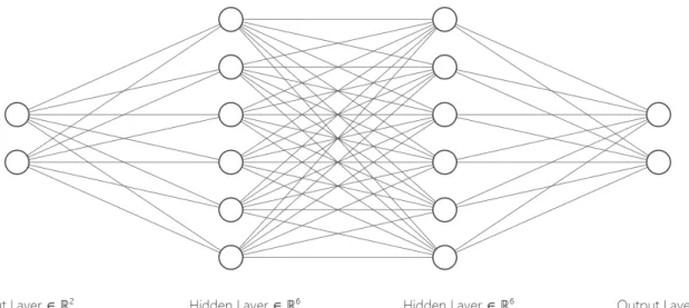
1.1 Fully Connected Neural Network . . . 2

2.1 GAN architecture . . . 6

2.2 Conditional GAN structure . . . 7

2.3 Convolutional Neural Network (LeNet[9]) . . . 8

2.4 Sigmoid function . . . 10

2.5 Tanh function . . . 11

2.6 ReLU function . . . 11

2.7 Leaky ReLU function . . . 12

2.8 Standard Neural Network . . . 16

2.9 Network with Dropout . . . 16

2.10 Residual Network[13] . . . 17

2.11 Transposed Convolution with a 2x2 kernel . . . 18

2.12 Fully Convolutional Network for Segmentation[15] . . . 20

2.13 Combining prediction from final layer and pool 4 layer . . . 20

3.1 MCDNN Network Architecture used to train patches of an image . . 22

3.2 Normal Encoder Decoder Network . . . 23

3.3 U-Net Generator . . . 24

3.4 Autoencoder Representation . . . 26

3.5 Multilayer Autoencoder[16] . . . 26

3.6 Encoder Decoder with ResNet block . . . 27

3.7 Linear Supervised Autoencoder . . . 29

3.8 Deep Supervised Autoencoder . . . 30

3.9 Semi Supervised Autoencoder . . . 31

3.10 VGG16 architecture . . . 33

4.1 Scatter Plot for table 4.1 . . . 37

4.2 Histogram for Table 4.1 . . . 37

4.3 Scatter Plot for table 4.2 . . . 39

4.4 Histogram for table 4.2 . . . 40

Chapter 1

Introduction

Over the past few decades, humongous amounts of data has been collected and made accessible with the help of digital revolution. A large part of today’s research involves extracting meaningful information from massive amounts of data including techniques like Machine Learning, Deep Learning, Data Mining,etc.

Machine Learning is the technique of designing a machine that can learn from data. A wide variety of Machine Learning Algorithms are utilised to train a ma-chine using data rather than writing custom code for a specific problem. Mama-chine Learning can be categorized into Supervised Learning, Unsupervised Learning and Reinforcement Learning (RL). Supervised Learning is divided into Regression and Classification problems. A regression problem is one in which we are trying to pre-dict results within a continuous output whereas in a classification problem, we try to predict results in a discrete output. Unsupervised Learning involves finding important trends in the data using clustering, feature extraction, dimensionality reduction,etc.

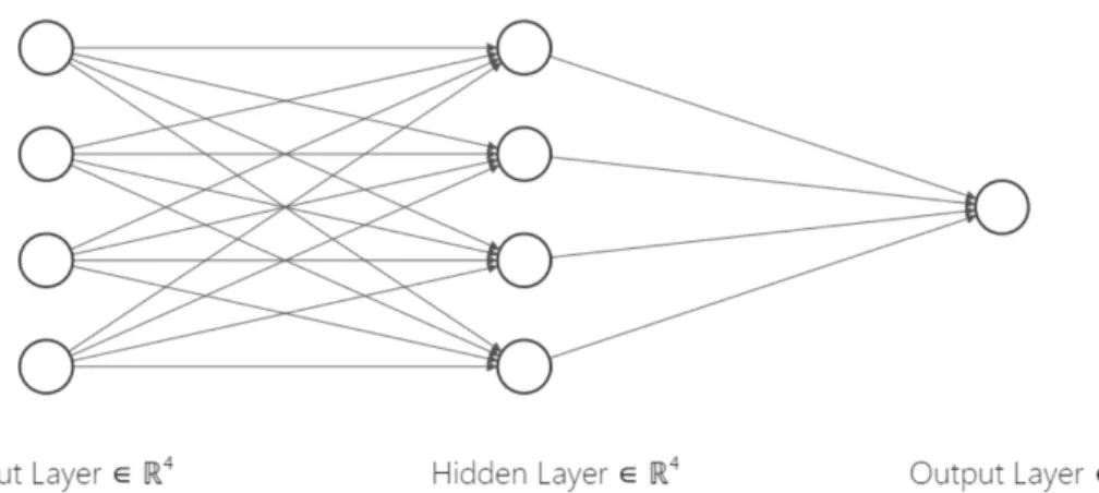
Deep Learning or Deep Neural Networks (DNN), a subset of Machine Learn-ing, utilizes multiple layers to extract features from data. These deep architecture networks have applications in Computer Vision, Speech Recognition, Machine

Trans-Figure 1.1: Fully Connected Neural Network

lation, Natural Language Processing,etc. In this thesis, we are interested in Deep Learning using generative models for the synthesis of state of the art realistic images. Generative models are models that learn features from the existing data and generate new indistinguishable samples.

1.1

Related Work

Generative Adversarial Networks[1] have been a topic of research in Deep Learning for a long time now. There are quite a few variants of GANs that have been proposed and used for various purposes. This thesis uses Conditional GANs[2] which are extensions of GANs, in which the Generator and Discriminator are conditioned with some additional information which could be based on class labels. Deep

Con-volutional GANs, by Radford et al.in 2015[3], utilized ConCon-volutional Neural Network components for the Generator to map a 100x1 noise vector to an output which is 64x64x3. Least Squares GAN[4] uses least squares loss function instead of the sig-moid cross entropy loss. InfoGAN[5], an information-theoretic extension to GAN, is able to learn representations in an unsupervised manner. The condition in infoGAN is ’learned’ rather than manually giving it like Condition GAN. Generating High Reso-lution images is another area where GANs are used extensively. SRGAN[6] generates super resolution images by recovering photo-realistic textures from down sampled im-ages. The loss function in SRGAN consists of an adversarial loss and a content loss as well as implements a deep residual network. SimGAN[7] utilizes self-regularization with adversarial loss to refine the images produced by the generator and updates the discriminator using previous refined images enabling it to generate realistic images. A challenging problem in Computer Vision is synthesizing realistic images using text description. StackGAN[8] is used to generate 256x256 photo realistic images condi-tioned on text description. The StackGAN works in two stages wherein Stage-I GAN draws the colors and shape of the object based on the given text descriptions and Stage-II GAN builds on Stage-I results and text descriptions as inputs by generating high-resolution realistic images.

1.2

Contribution

This thesis explores the use of Generative Adversarial Networks for the gener-ation of images. We try to figure out the changes in the generated image based on the generator architecture and compare the performance with the already existing frame-works. In Chapter 2, we summarize the theory of Convolutional Neural Networks and GAN’s. In Chapter 3, we come up with the different Generator architectures and

summarize them in detail along with the results for each of them. In chapter 4, we extend the generator architecture by adding convolution layers to extract high level features in order to generate high resolution images.

Chapter 2

Background

2.1

Generative Adversarial Networks

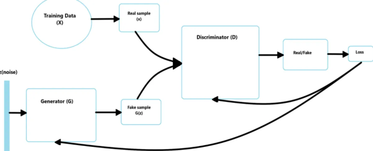
In 2014, Goodfellow et al. proposed Generative Adversarial Networks[1] which is a generative model consisting of a generator G and a discriminator D. The generator tries to generate images and the discriminator tries to distinguish between images drawn from the generator and the samples drawn from the training data.

The Generator takes a noise vector z and generates fake samples. The Dis-criminator takes the sample from the generator as well as the real sample from the training data. The generator and the discriminator play the following two player minimax game with a value function V(G,D):

Figure 2.1: GAN architecture

The cost function for the discriminator is given as:

1 m m X i=1 [log(D(xi)) + log(1−D(G(zi)))] (2.2)

It is calculated into two parts wherein the first part is loss for the real sam-ple(D(x) represents the probability that x came from the training data and the second part is the loss for the fake sample.

The cost function for the generator is given as:

1 m m X i=1 [log(1−D(G(zi)))] (2.3)

2.2

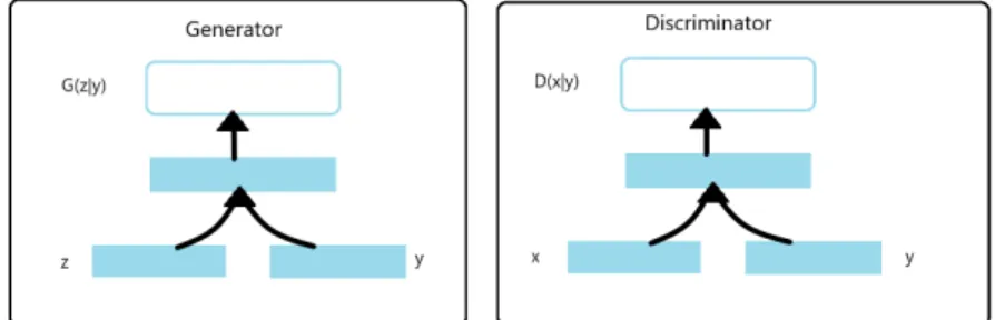
Conditional Generative Adversarial Network

The generated data by GANs can have various modes and in most of the cases it is desirable to have control over it. By conditioning the model on additional information in what is called a Conditional GAN[2], it is feasible to direct the data

Figure 2.2: Conditional GAN structure

generation process. The applied conditioning can be based on class labels or data from different modality.

The objective function of Conditional GAN is

minGmaxDV(D, G) =Ex∼pdata(x)[log(D(x|y))] +Ez∼pz(z)[log(1−D(G(z|y))] (2.4)

In the generator, the noise(z) and y are combined and in the discriminator x and y are combined.

2.3

Convolutional Neural Network

Convolutional Neural Network are a type of feed forward neural networks that are used to find patterns in an image by convolving over it. The first few layers of a CNN can identify lines and corners. By passing these lines and patterns down through our neural network (the latter layers), we can recognize more complex features. Generally, the convolution layers are followed by fully connected layers

Figure 2.3: Convolutional Neural Network (LeNet[9])

like in a multilayer perceptron. The convolution layers have various advantages when compared to a normal feed forward neural network. A feature detector (kernel) which is useful in one part of the image, is also useful in other parts of the image. The output value in each layer depends on a small number of inputs.

The convolutional neural network also consists of Pooling layers. Max pooling can be defined as

mi = max

∀s∈Sjqs (2.5)

Average pooling can be defined as

1 n n X ∀s∈Sj qs (2.6)

where q is some pixel in the sub region Sj from the the feature mapping and

n is the number of features. These layers help in dimensionality reduction and helps in position invariant feature extraction.

2.4

Activation Function

In order for a neural network to learn non linear transformations, we require activation functions. If we do not use an activation function, the neurons would sim-ply do a linear transformation using weights and bias which will hinder the capacity of the network to learn complex functional mappings. There are four major activa-tion funcactiva-tions that are predominantly used namely Sigmoid, Tanh, ReLU and Leaky ReLU.

2.4.1

Sigmoid

:

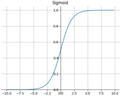
Sigmoid function has a ’S’ shaped curve. The output of sigmoid is in the range (0,1).

hθ(x) = 1

1 +e−z (2.7)

In deep neural networks, using sigmoid activation function leads to vanishing gradient problem where the gradient value in the initial layers decreases greatly and the preceding layers train very slowly or with extremely low gradients.

2.4.2

Tanh

:

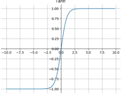
Tanh activation function can be viewed as the rescaled version of the sigmoid function. The output of tanh is in the range (-1,1). It is given by the formula

hθ(x) =

ez−e−z

Figure 2.4: Sigmoid function

2.4.3

ReLU (Rectified Linear Unit)

:

ReLU is defined as:

y= max(0, x) (2.9)

This activation function allows our network to converge quickly thereby mak-ing it computationally efficient.

If the inputs are negative, the gradient of the function becomes zero and the network cannot perform backpropagation which is a disadvantage of ReLU.

2.4.4

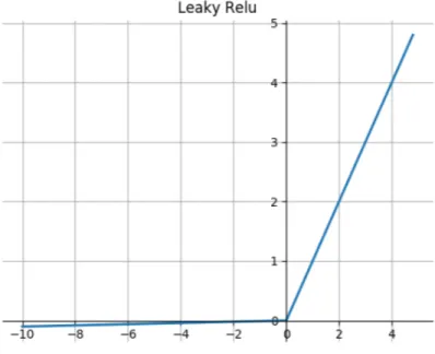
Leaky ReLU

Figure 2.5: Tanh function

Figure 2.7: Leaky ReLU function

The Leaky ReLU is different from ReLU in that it has a small slope in the negative direction so as to prevent the gradients from becoming zero when the inputs are negative.

y= max(0.01x, x) (2.10)

2.5

Methods of Training

2.5.1

Batch Gradient Descent

In batch gradient descent, each gradient step uses all the training examples. Since the entire dataset is used to compute gradients, there is room for redundant

computations as it recomputes gradients for similar examples.

θ=θ−η.∇θJ(θ) (2.11)

As we need to calculate the gradient of the entire dataset to make an update, batch gradient descent can be very slow. Another disadvantage of batch gradient descent is that it does not allow us to update our model with new examples on the fly.

2.5.2

Stochastic Gradient Descent

Stochastic Gradient Descent[10] uses a single example to compute and update the gradient of parameters. SGD does not recompute gradients for similar examples and hence, there is no room for redundant computations.

θ =θ−η.∇θJ(θ;x(i);y(i)) (2.12)

Since, SGD uses a single example to compute gradients, frequent updates are performed and hence, it is faster.

2.5.3

Mini Batch Gradient Descent

Mini Batch Gradient Descent combines batch gradient descent and stochas-tic gradient descent and computes gradients for mini batch of size commonly taken between 50 and 250.

θ=θ−η.∇θJ(θ;x(i:i+n);y(i:i+n)) (2.13)

both worlds.

2.5.4

Backpropagation

Backpropagation is a common technique for training neural networks in which the weights of the connections are repeatedly adjusted so as to minimize the difference between actual output and the output of the network. First, the loss associated with the prediction is calculated and all the losses summed up to compute the final error. This error is the back propagated and the partial derivatives of the loss function are computed for all weights w and biases b associated with the network.

2.6

Batch Normalisation

A deep neural network is difficult to train because each layer’s input depends on the parameters of the previous layers and hence, small changes to the network parameters amplify as the network becomes deeper. This results in a change in the distribution of the network activations which is knows as internal covariate shift. Covariate shift can also be explained as suppose we train our network on images of black horses only. If we now try to apply this network to data with colored horses, it will not do well. In other words if we are training our network to learn a mapping from X to Y and if the distribution of X changes, then we might need to retrain our network to adapt to the distribution of X. This problem is addressed by normalizing inputs. The resulting neural network after batch normalisation is robust as they are less prone to divergences caused by the choice of initializations or from faster learning rates being used for the network.

Batch normalisation[11] works because the input features after normalization are in a specific range and this happens not just for the input layer but also for

hidden units as well. An example of this is if we have a neural network with eight hidden layers and we look at the fourth hidden layer. So what it does is it will limit the amount to which updating the parameters in the earlier layers(first, second and third here) can affect the distribution of values of the fourth layer. Also, if we train our network using a mini batch algorithm, each time we scale the mini batch by the computed mean/variance which in adds some noise to the mini batch. This has a slight regularization effect similar to dropout. This regularization effect can be reduced by using larger mini batch size.

2.7

Dropout

Since the advent of deep neural networks, there are multiple hidden layers used to learn complicated mappings from input to output which might not be present in the test data. This leads to overfitting wherein the network performs well with the training data but does not perform well with the test data. Also with larger neural networks, we can also average the predictions of seperately trained network but in essence, this is an expensive computation. Training several models also poses the problem of selection of optimal hyperparamters. These problems can be solved with the help of dropout[12]. The term dropout refers to dropping some units in both a hidden as well as visible layer randomly.

When we dropout a unit, we temporarily remove it from the network along with its incoming and outgoing connections. The dropping of units occurs randomly with the probability of each unit being retained is p. In this manner, we are also able to train a number of networks using just one network by sampling a smaller network from a bigger network. Another advantage of dropout is that if the activation of a particular neuron in a hidden layer is high, the corresponding outgoing connection

Figure 2.8: Standard Neural Network

Figure 2.10: Residual Network[13]

and the subsequent neuron can become overly dependent on it. Dropout solves this by negating this problem as this high activation neuron could be turned off at any time thereby preventing overfitting. At test time, we use a single neural network without dropout by making slight changes. If we retain the weight with a probability p, the outgoing weights of that unit are multiplied by p at test time which ensures that the expected value is met.

2.8

Residual Networks

As the number of layers in a neural network increase, the accuracy of the network gets improved as it can extract high level features in addition to the low level features. Hence, the deeper models are better feature extractors than there shallow counterparts. But as the number of layers increase, the network can suffer from vanishing gradient problem. To counter this, we add skip connections to the network.

Figure 2.11: Transposed Convolution with a 2x2 kernel

connected and pooling layers. The shortcut connections which perform identity map-ping neither add to the number of learnable parameters nor the computation com-plexity. The changed network can be trained end to end with Stochastic Gradient Descent with backpropagation.

2.9

Transposed Convolution

In 2010, Zeiler et al. introduced the concept of Transposed Convolution[14] (also called Deconvolution). Many examples from Computer Vision utilize Trans-posed Convolutions which involves a series of normal convolutions to compress the input data and then decompressing it to get something meaningful. Transposed Con-volutions differ from Bicubic Interpolation and other upsampling methods in that they require kernel weights to be learned thereby increasing the number of learnable parameters. In general, it can be thought of as going in the opposite direction to normal convolution.

The deconvolution network used for semantic segmentation uses unpooling and deconvolution. The unpooling layers perform the reverse of the pooling layers

and reconstructs the original size of activations. The deconvolution layers densify the sparse activations obtained by unpooling by generating multiple outputs from a single input.

2.10

Fully Convolutional Network

When we use convolutional neural network for classification, the input image goes through the convolution, pooling and fully connected layers and output a pre-dicted label for the input image. The presence of fully connected layers in a CNN means that it takes fixed sized inputs and produce non spatial outputs.However, the fully connected layers can be transformed into convolution layers which yields a fully convolution network that can take input of any size and outputs a classification map. While fully convolutionized networks perform well in segmentation, the sheer length of the network makes it lose the spatial location information and renders the output rough.

To solve the problem of rough output, a skip connection can be added that combines the final prediction layer with lower layers.

Figure 2.12: Fully Convolutional Network for Segmentation[15]

Chapter 3

Research Design and Methods

In this chapter, we define different approaches that we take in order to train a GAN. The generator which is used to generate images close to real data can have different architectures and we demonstrate the efficiency of each. The discriminator that we adopt is the 70x70 patch discriminator for each generator architecture. We domonstrate the importance of a loss function and its impact on the generated images. The choice of hyperparameters is essential to the success of any network as they determine the network structure. We employ U-NET architecture as the generator with the discriminator being 70x70 patch discriminator. We then employ ResNet blocks along with encoder and decoder as the generator with the discriminator being the same. The third generator architecture we use is the SegNet architecture along with the ResNet blocks.

3.1

U-Net as a Generator

Convolutional networks are typically used in classification tasks, where they output a single class label for an input image. In semantic segmentation tasks, there

Figure 3.1: MCDNN Network Architecture used to train patches of an image

is a need that a label should be assigned to each pixel of the image. In Biomedical tasks, collecting huge number of images to train the network is a very difficult task. Discovering nuclei of cells requires the use of various kinds of dyes and collecting thousands of image for training can be beyond reach. In 2012, Ciresan et al.[16] trained a network to predict class label of each pixel using the sliding window setup. He provided a local region(patch) around that pixel to train for every pixel which helped in the localization of the prediction. The number of patches used for training can be more as compared to the number of images that can be used for training thereby resulting in more data.

The major drawback of the technique used by Ciresan et al. is that it is extremely slow since the network has to be trained on various number of patches. Training on patches also leads to a lot of redundancy in calculations due to overlap-ping. Since the patch is not consistent, larger patches can require more max-pooling layers thereby leading to a reduced localization accuracy.

Figure 3.2: Normal Encoder Decoder Network

The U-Net[17] architecture builds on the fully convolutional network architec-ture. The U-NET generator consists of a usual compressing network which is similar to having convolution layers one after the other. By doing this, we will have a higher level representation of the data after the final encoding layer. This is followed by a series of upsampling layers for increasing the resolution of the output.

The U-NET differs from the normal encoder decoder network such that the high resolution features from the compressing path are combined with the upsampled output i.e it consists of skip connections connecting encoder layers to decoder layers. The upsampling part consists of a large number of feature channels which makes it possible for the network to send the context information to higher resolu-tion layers which also makes the upsampling part symmetric to the compressing or downsampling part giving it a u-shaped architecture. With each skip connection, we concatenate all channels at layer i with those at layer n-i. The network does not consist of fully connected layers and only uses convolution layers which means the

Figure 3.3: U-Net Generator

segmentation map only contains pixels for which the full context is available in the input image.

The architecture employed consists of 16 hidden layers that can be divided into (i) an encoder which downsamples the image and evaluates feature maps at multiple scales thereby yielding a multilevel, multiresolution feature representation, and (2) a decoder that upsamples the image taking in the extracted feature representation by the encoder and classifies pixels at original image resolution. The encoder consists of replicating application of one convolution using a kernel size of four with padding and stride two halving the resolution of the resulting feature map, each followed by a leaky rectified linear unit with a leakage factor of 0.2. The decoder consists of replicating transposed convolutions with a kernel size of four with padding and stride two doubling the resolution of the resulting feature map. At the final layer, tanh activation function is used.

3.2

Encoder Decoder with ResNet

Neural networks are specialized in converting high dimensional data to low dimensional data via a series of stacked layers. Dimensionality reduction is the basis for visualization and classification of high dimensional data. However, we face diffi-culties if the available dataset is small or liable to suffer from noise. There are quite a few ways to resolve the problem of model overfitting with one being the complexity of the model and another being increasing the training data. Changing the neural network architecture have long been one of the favorite methods to reduce overfitting which includes adding layers or changing models. Dropout is an effective technique that has long been used to avoid overfitting where a part of the network is removed randomly in every pass which prevents overfitting. Most of these methods are based on high amount of training data. The Encoder Decoder network which are also knows as Autoencoders are trained on relatively small datasets and are based on ideas which have been there in the form of implementations of lossy compression. Training an autoencoder can be done by normal raw data and these are considered as unsuper-vised learning technique as they do not require explicit labels and generate there own labels.

Principal Component Analysis (PCA) is a technique that has long been used to convert high dimensional data to low dimensional data which recognizes the directions of high variance and represents data points in each of these directions. Autoencoders can be used as a substitute to methods like principal component analysis where an encoder network transforms high dimensional data to low dimensional data and an identical decoder network to recover the data from the code.

Both the encoder and decoder start with random weights which are then trained together using an objective function with an aim to reduce the

inconsis-Figure 3.4: Autoencoder Representation

Figure 3.6: Encoder Decoder with ResNet block

tency between original data and its reconstruction. In a bid to outperform PCA, autoencoders can work on non linear data where the number of layer in the network are equivalent or more than the dimensions of the data. Autoencoders have also been employed as a tool to improve supervised learning by running in parallel as a tuning denoising tool that provides input which is added to the supervised learning input in the final layer.

The autoencoder model employed consists of two symmetrically inverted mod-els of encoder and decoder. The input dimensions are the same as the output dimen-sions. Batch Normalization is present after every convolution and transposed convo-lution operation. We have ReLU activation function. There are 9 ResNet blocks used with 2 convolution layers per ResNet block. The final decoder layer is followed by a convolution layer and tanh activation function.

of which being layer wise training[17] and the use of auxiliary variables for hidden layers. One such auxiliary task model is the supervised autoencoder which has shown to provide noteworthy improvements when used in deep neural networks. Supervised autoencoders are trained on data

[x1, y1],[x2, y2]...[xn, yn]

with the aim to predict well on new samples generated from the same input. The key here is that the new samples are generated using the same data that we train the network on. Keeping this in mind, we transform the data into a new representation. Autoencoders are extensively used to extract meaningful transformations. The output of the autoencoder is set to input, x. The autoencoder learns to reconstruct the input and in the process extracts underlying or abstract attributes that help in the accurate prediction of the inputs.

A supervised autoencoder is one which contains the addition of a supervised loss on the representational layer. If there is a single hidden layer in the network, then a supervised loss is added to the output layer. If we have a deep autoencoder, the innermost (smallest) layer would have a supervised loss added to it. The addition of supervised loss has the advantage of driving representation learning towards tasks that are desired. Solely training a neural network by learning a hidden layer is an under constrained task which will find solutions that fit the data very well but is unable to find the underlying patterns in the data. In 2017, Deng et. al. introduced the Semi Supervised autoencoder (SS-AE) which is based on the blend of supervised learning and unsupervised learning. Just like the general supervised autoencoder, the semi supervised autoencoder can contain several hidden layers with the encoder trying to extract high-order features and the decoder trying to reconstruct the data.

Figure 3.7: Linear Supervised Autoencoder

The idea is to make the coded features contain all the important information of the original data.

The equations for the semi supervised autoencoder when the coding and de-coding parts have only one layer can be expressed as

Y =S(W1∗X+B1)[CodingP art] (3.1)

Z =S(W2∗Y +B2)[DecodingP art] (3.2)

where S is the activation function, W1 and W2 are the weight matrices, B1 and B2 are the biases, Y is the encoded data and Z is the output of the decoder. Semi supervised autoencoders have further been improved by replacing the original activation function

Figure 3.8: Deep Supervised Autoencoder

being used by Elu and then adding dropout to each layer of the network as well as linking the classifier directly to the encoder. The general activation functions are replaced by Elu because with ReLU and sigmoid, when the input is negative or large negative values,the output of the hidden nodes becomes 0. Dropout is added to every layer to shut some of the units in a hidden layer randomly so as to prevent overfitting.

3.3

Objective Function

The objective function of a conditional GAN can be summed up as

Figure 3.9: Semi Supervised Autoencoder

where G tries to minimize this objective function against an adversary D that tries to maximize it. There have been quite a few approaches where GAN objective has been mixed with L2 distance. The job of the discriminator is the same but the job of the generator is to produce images that are close to the ground truth in an L2 distance sense. In our experiments, we have instead tries L1 distance because L2 distance caused blurring.

L1(G) = Ex,y,z||y−G(x, z)||1 (3.4)

The final objective can be states as

Without including z, the network would still learn the mapping from x to y but would produce deterministic outputs. In our model, we provide only in the form of dropout applied on several layers of our generator at both training and test time. Designing the conditional GAN such that it captures the full entropy of the conditional distribution it is trying to emulate is an important task.

3.4

SegNet with ResNet as a Generator

SegNet with ResNet is the third generator architecture used in our experi-ments which is a deep fully convolutional neural network for the purpose of semantic pixel wise segmentation. The architecture consists of an encoder network, a decoder network followed by a pixel wise classification layer. The decoder upsamples using the pooling indices generated at the max pooling layer with an aim to map the low resolution feature maps to full input resolution feature maps which eliminates the need of learning to upsample. These upsample maps are then convolved with train-able filters to produce dense feature maps. The architecture of our encoder network is based on the VGG16 [] network.

The encoder network does not contain the fully connected layers in a VGG16 which makes the SegNet encoder which makes the network extremely small and easier to train[]. The important component of our encoder is the decoder which corresponds to each encoder in use. The decoder uses max-pooling indices which are saved at the time of using max-pool layer in the encoder to execute non linear upsamping. There are quite a few advantages of using max-pooling indices like

• It can be used in any encoder decoder architecture • It reduces the number of trainable parameters

The encoder network constitutes 13 convolutional layers which are the first 13 convolutional layers of a VGG16 network. Each encoder layer has a corresponding decoder layer which means there are 13 decoder layers. The encoder layers perform convolution to generate feature maps which is then followed by bath normalisation and rectified linear unit (ReLU) activation function. Then a max pooling of 2x2 window and stride 2 is performed and the resulting output is subsampled by a factor of 2. Max pooling layers help in achieving translational invariance. While several max pooling and sub sampling layers provide translational invariance, it leads to a loss of spatial resolution of the feature maps which invariably leads to lossy boundary details which is extremely undesirable for segmentation tasks. Hence, it is important to capture and store boundary information. In this work, we store the boundary information in the form of max pool indices which is the location of the maximum feature value. These maximum feature value are remembered after each pooling operation. The decoder employed in the network then uses the max pooling indices to upsample the input feature map from the corresponding encoder feature map. This happens without learning. These feature maps are then convolved with the trainable decoder filter bank which is followed by batch normalisation. The last encoder block is followed by a resnet block which is included to learn the important features from the low dimensional data. The input to the encoder is a grayscale image (1 channel) and the decoders in the network produce feature maps with the same number of size and channels as there corresponding encoders.

Chapter 4

Results

Generator Average difference in cell

count

Standard Deviation

Encoder Decoder with ResNet 15.2 10.66

UNeT 21.7 17.28

SegNet 46 25.62

Encoder Decoder with ResNet for High Resolution

6.42 4.89

We evaluated the results by using different generator architectures. The above results are for dataset with 4616 number of training images. The Encoder Decoder with ResNet has average difference in cell count 15.2 and the standard deviation 10.66. The average value of pearson correlation coefficient for the same has an average value of 0.86. The number of downsampling layers in the encoder is 2 and the same number of layers will be in the decoder. Our setting has lambda equal to 300. The size of the feature maps is 3*3 and we use a stride of 2. The activation function used after every convolution layer is ReLU and a tanh activation function at the end. The network is

Table 4.1: Encoder Decoder with ResNet Case Count Real Count Fake Difference

1 414 263 151 2 379 333 46 3 195 155 40 4 161 151 10 5 226 163 63 6 125 145 20 7 162 183 19 8 57 68 11 9 163 151 12 10 123 148 25

trained for 200 epochs. The encoder decoder with resnet was also used for single cell lines before the combined dataset and the results are as follows:

The training data for this single cell has 864 images and the highest average difference in cell count is 151. The difference for all the other images gives a mean of 27.99. The cell count of the real image for which the difference is 151 is 414 in turn is a lot more when compared to the other images.

Figure 4.1: Scatter Plot for table 4.1

Table 4.2: UNet as Generator

Case Count Real Count Fake Difference

1 414 233 181 2 379 293 86 3 195 138 57 4 161 142 19 5 226 134 92 6 125 124 1 7 162 154 8 8 57 62 5 9 163 107 56 10 123 125 2

The histogram for table 4.1 shows that there are 6 images for which the dif-ference in cell count is between 0-39, 3 images for which the difdif-ference in cell count is between 40-79 and 1 image for which the difference in cell count is between 120-159(highest).

The average difference in cell count for UNeT architecture for the dataset with 4616 training images is 21.7 and standard deviation of 17.28. There are 8 encoder layers and corresponding 8 decoder layers. There are skip connections between en-coder layer and the corresponding deen-coder layer. The feature maps of size 4*4 are used along with a stride of 2. The UNeT architecture was also examined on single cell line of training images 864 and the results are as follows:

The average difference in cell count is 50.7. The highest difference in cell count is 181 where the cell count in the real image is 414. The average for the rest of the 9 images is 36.22.

Figure 4.4: Histogram for table 4.2

The histogram for table 4.2 shows that there are 5 images for which the dif-ference in cell count is between 0-29, 2 images for which the difdif-ference in cell count is between 30-59, 1 image for which the difference in cell count is between 60-89, 1 image for which the difference in cell count is between 90-119 and 1 image for which the difference in cell count is between 180-209.

The third architecture which is the SegNet architecture has an average differ-ence of cell count for the dataset with 4616 training images to be 46 and 25.62. The network runs for 200 epochs and uses ReLU activation function after every convolu-tion layer. The SegNet architecture was also test for single cell line qith 864 training images and the results are as follows:

Table 4.3: SegNet with ResNet as Generator Case Count Real Count Fake Difference

1 414 306 108 2 379 287 92 3 195 156 39 4 161 109 52 5 226 192 33 6 125 119 6 7 162 133 29 8 57 29 28 9 163 105 58 10 123 97 26

The average difference in cell count is 47.1. The highest difference in cell count is 108 where the cell count in the real image is 414. The difference here is very consistent for all the images. Our architecture consists of 13 convolution layers like the first 13 convolution layers of VGG16 architecture and another 13 convolution layers in decoder. Every convolution layer is followed by batch normalisation and ReLU activation funtion. The size of kernel used is 3*3 with a padding of 1 in the convolution layers. The maxpool layer has a kernel size of 2*2 with a stride of 2. While applying maxpool, the indices are saved which are later used for upsampling.

Figure 4.5: Histogram for table 4.3

The histogram for table 4.2 shows that there are 5 images for which the dif-ference in cell count is between 6-35, 3 images for which the difdif-ference in cell count is between 36-65, 1 image for which the difference in cell count is between 66-95 and 1 image for which the difference in cell count is between 96-125.

Chapter 5

Conclusion

In this thesis, we studied GAN, in particular Conditional GAN and how var-ious changes in its architecture impact the image generation. We try to generate nuclei stained images by using different GAN generator architectures. The major architecture involves around having an encoder to extract high level features and a corresponding decoder to reconstruct the image. The process of feature extraction is made even more prominent by having a series of residual blocks after the encoder. The batch size with which the images are fed to the network is 1, which is used for low as well as high resolution image generation. By using various metrics to measure the accuracy of the generated images, we found that the encoder decoder with resnet as a generator works better than UNeT and SegNet as generators. The results are generated using Cell Profiler software where the cell count is obtained for the real and the fake(generated) images and the difference between the two is evaluated.

Chapter 6

References

[1] Goodfellow, Ian, et al. ”Generative Adversarial Nets.” Advances in Neural Information Processing Systems. 2014.

[2] Mehdi Mirza and Simon Osindero. ”Conditional Generative Adversarial Nets.” arXiv preprint arXiv:1411.1784(2014)

[3] Radford, A., Metz, L. and Chintala, S. ”Unsupervised representation

learn-ing with deep convolutional generative adversarial networks.” arXiv preprint arXiv:1511.06434, 2015.

[4] Mao, X., Li, Q., Xie, H., Lau, R. Y. and Wang, Z. ”Least squares generative adversarial networks.” arXiv preprint arXiv:1611.04076, 2016.

[5] Chen, X., Duan, Y., Houthooft, R., Schulman, J.,Sutskever, I., and Abbeel,

P.”InfoGAN: Interpretable Representation Learning by Information Maximizing.”Generative Adversarial Nets. ArXiv e-prints, June 2016

[6]Ledig, C., Theis, L., Huszar, F., Caballero, J., Aitken, A. Tejani, A. Totz, J. Wang, Z. and Shi, W. ”Photo-realistic single image super-resolution using a generative adversarial network.” In CVPR, 2017

R. ”Learning from simulated and unsupervised images through adversarial training.” arXiv preprint arXiv:1612.07828, 2016.

[8] Zhang, H., Xu, T., Li, H., Zhang, S., Huang, X., Wang, X. and Metaxas, D.”StackGAN: text to photo-realistic image synthesis with stacked generative adver-sarial networks.” In ICCV, 2017

[9] LeCun, Y., Bottou, L., Bengio, Y. and Haffner, P. ”Gradient Based Learn-ing applied to document recognition”. ProceedLearn-ings of the IEEE, 86(11):2278-2324, November 1998a

[10]Bottou, L., Frank E. and Nocedal, J., ”Optimization Methods for Large Scale Machine Learning”. arXiv preprint arXiv:1606.04838(2016)

[11]Ioffe, S. and Szegedy, C. ”Batch Normalization: Accelerating deep network training by reducing internal covariate shift”. In ICML, 2015.

[12]Srivastava, N., Hinton, G., Sutskever, A., Sutskever, I. and Salakhutdinov, R. ”Dropout: A simple method to prevent neural networks from overfitting”. J Mach. Learn. Res., 15(1):1929-1958, January 2014.

[13] He, K., Zhang, X., Ren, S. and Sun, J., ”Deep residual learning for image recognition”. In CVPR, 2016.

[14] Zeiler, Matthew D., et al. ”Deconvolutional networks.” Computer Vision and Pattern Recognition(CVPR),2010 IEEE Conference on. IEEE, 2010.

[15] Long, J., Shelhamer, E. and Darrell, T.”Fully convolutional networks for semantic segmentation.” In CVPR, 2015.

[16] Ciresan, D. C., Giusti, A., Gambardella, L. M. and Schmidhuber, J.”Deep neural networks segment neuronal membranes in electron microscopy images.” In NIPS,2012.

[17] Fischer, P., Dosovitskiy, A. and Brox, T.”Descriptor matching with con-volutional neural networks: a comparison to SIFT.” CoRR, abs/1405.5769, 2014.