Convolutional Neural Networks for Land-cover Classification Using Multispectral Airborne Laser Scanning Data

(1)

Convolutional Neural Networks for Land-cover

Classification Using Multispectral Airborne

Laser Scanning Data

by

Zhuo Chen

A thesis

presented to the University of Waterloo in fulfillment of the

thesis requirement for the degree of Master of Science

in Geography

Waterloo, Ontario, Canada, 2018

(2)

AUTHOR'S DECLARATION

I hereby declare that I am the sole author of this thesis. This is a true copy of the thesis, including any required final revisions, as accepted by my examiners.

(3)

Abstract

With the spread of urban culture, urbanisation is progressing rapidly and globally. Accurate and update land cover (LC) information becomes increasingly critical for protecting ecosystems, climate change studies and sustainable human-environment development. It has been verified that combining spectral information from remotely sensed imagery and 3D spatial information from airborne laser scanning (ALS) point clouds has achieved better LC classification accuracy than that obtained by using either of them solely. However, data fusions can introduce multiple errors. To solve this problem, multispectral ALS developed recently is able to acquire point cloud data with multiple spectral channels simultaneously. Moreover, deep neural networks have been proved to be a better option for LC classification than those statistical classification approaches.

This study aims to develop a workflow for automated pixel-wise LC classification from multispectral ALS data using deep-learning methods. A total of six input datasets with a multi-tiered architecture and three deep-learning classification networks (i.e. 1D CNN, 2D CNN, and 3D CNN) have been established to seek the optimal scheme that lead to highest classification accuracy. The highest overall classification accuracy of 97.2% has been achieved using the proposed 3D CNN and the designed input dataset. In regard to the proposed CNNs, the overall accuracy (OA) of the 2D and 3D CNNs was, on average, 8.4% higher than that of the 1D CNN. Although the OA of the 2D CNN was at most 0.3% lower than that of the 3D CNN, the run time of the 3D CNN was five times longer than the 2D CNN. Thus, the 2D CNN was the best choice for the multispectral ALS LC classification when considering efficiency. For different input datasets, the OA of the designed input datasets was, on average, 3.8% higher than that of the classic input datasets. Results also showed that the multispectral ALS data is superior to both multispectral optical imagery and single-wavelength ALS data for LC classification. In conclusion, this thesis suggests that LC classification can be improved with the use of multispectral ALS data and deep-learning methods.

(4)

Acknowledgements

First and foremost, I would like to express my deepest appreciation to my supervisor, Professor Dr. Jonathan Li, whose contribution in stimulating suggestions and encouragement helped me to coordinate my graduate studies especially in completing this thesis. I feel very fortunate that he provided me the opportunity to get involved in and work on state-of-the-art technologies, especially the multispectral LiDAR and deep learning. I am deeply grateful for his guidance and support throughout my graduate studies.

I would like to thank my thesis committee members, Dr. Michael Chapman, Professor at the Department of Civil Engineering, Ryerson University, Dr. Peter Deadman, Associate Professor at the Department of Geography and Environmental Management, University of Waterloo, and Dr. John Zelek, Associate Professor at the Department of Systems Design Engineering, University of Waterloo, for reviewing my thesis, serving as my thesis examining committee, and providing me the constructive comments and valuable suggestions.

Furthermore, I would like to acknowledge Teledyne Optech for providing me the datasets acquired by their multispectral ALS system TITAN to support my study. I would like to thank staffs in the department of Geography and Environmental Management, especially Alan Anthony and Susie Castela, for their help. My sincere thanks also go to Zilong Zhong, Lingfei Ma, Ying Li, Ming Liu, Weiya Ye, Yue Gu, and Mengge Chen, all the members in Mobile Sensing and Geodata Analytics Lab, who shared their experiences during the group meetings and created a delightful environment in the office. A special thanks goes to Yuhao Xie for providing me advice on the studies of Python and deep learning.

Last but not least, I would like to express deepest gratitude to my dear parents for their unconditional love, support and emotional encouragement throughout my studies. I could not be more grateful for having such wonderful parents. Thanks to my boyfriend, Hao Wu, and my friends, Liuyi Guo, Bo Sun, Michael Guo, Yuhao Xie, and Hongjing Chen, who accomplish me and offer me with their help, understanding, and encouragement.

(5)

List of Figures

Figure 2.1 Titan laser channels with spectral signatures for selected objects (Teledyne Optech

Titan, 2015) ... 7

Figure 2.2 Optech Titan system (Teledyne Optech Titan, 2015) ... 8

Figure 2.3 Cooperation principle of GNSS and IMU (Chen et al, 2018) ... 10

Figure 2.4 Structure of Standard Deep Neural Network ... 19

Figure 2.5 the Relationship among Deep Learning, Machine Learning, Representation Learning, and Artificial Intelligence (Goodfellow et al., 2016) ... 20

Figure 2.6 the Relationship among Deep Learning, Machine Learning, Representation Learning, and Rule-based Systems (Goodfellow et al., 2016) ... 21

Figure 2.7 Category and Representative Examples of Deep Learning Algorithms ... 22

Figure 2.8 Comparisons among Four Categories of Deep Learning Algorithms. ... 24

Figure 3.1 A map of the study area ... 30

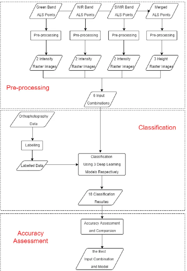
Figure 3.2 Workflow of the methodology ... 34

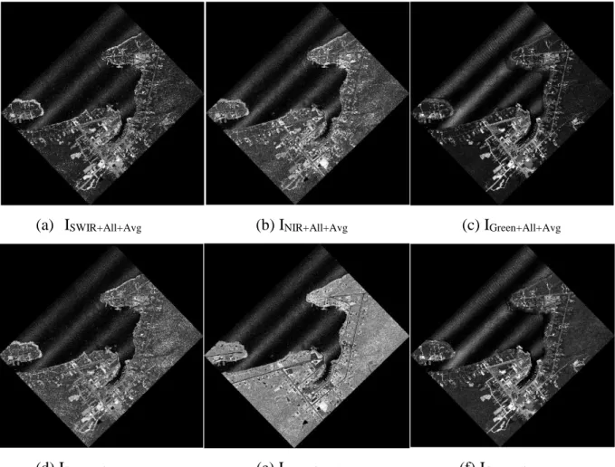
Figure 3.3 Multispectral ALS on the study area ... 37

Figure 3.4 Multispectral ALS height models on the study area ... 38

Figure 3.5 Multi-tiered architecture of input datasets ... 40

Figure 3.6 Structure of CNNs ... 42

Figure 3.7 Establishment of CNNs ... 43

Figure 3.8 Workflow of model implementation ... 46

Figure 3.9 Imported libraries ... 47

Figure 3.10 Importing data pixel by pixel ... 47

Figure 3.11 Selection of valid pixels ... 48

Figure 3.12 Separation of Training and Testing Data ... 48

Figure 3.13 A forward step and a backward step of training process ... 49

Figure 3.14 Training process ... 49

Figure 3.15 Predict process ... 50

Figure 4.1 Labelled LC map of the study area ... 55

Figure 4.2 Results of different shape of input unit in 2D and 3D CNNs ... 58

(9)

Figure 4.4 Results of different size of kernels in the 1D, 2D and 3D CNNs ... 60

Figure 4.5 Results of different size of kernels in the 1D, 2D and 3D CNNs ... 61

Figure 4.6 Results of different units of dense in the 1D, 2D and 3D CNNs ... 62

Figure 4.7 Results of different units of dense in the 1D, 2D and 3D CNNs ... 63

Figure 4.8 Predicted maps of different input data combinations with the 3D CNN ... 66

(10)

List of Tables

Table 2.1 Specifications of Titan... 7

Table 2.2 Studies Related to Multispectral ALS Data Classification ... 13

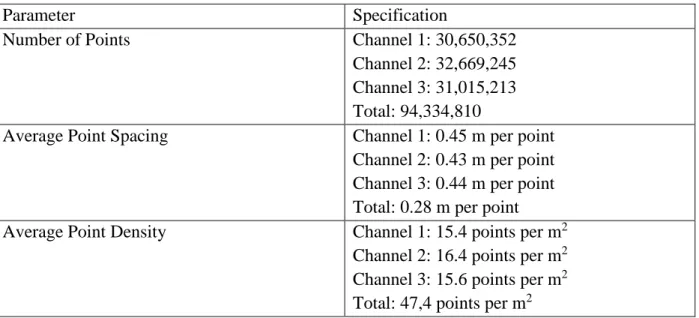
Table 3.1 Summary of data collection parameters ... 32

Table 3.2 Summary of the cropped, pre-processed and merged data ... 32

Table 3.3 Content of input combinations ... 40

Table 3.4 LC types and examples... 41

Table 3.5 Hyper-parameters involved in the establishment of models ... 45

Table 3.6 Hyper-parameters involved in the implementation of CNNs ... 50

Table 3.7 An example table of a confusion matrix with UA and PA ... 51

Table 4.1 Detailed examples of each LC class in labelled dataset ... 56

Table 4.2 Statistics of the labelled dataset ... 56

Table 4.3 Confusion matrix of first-labelled dataset and relabelled dataset ... 57

Table 4.4 Summary of hyper-parameters ... 63

Table 4.5 OA and kappa coefficient of each model ... 65

Table 4.6 Confusion matrix for Combination 1 with the 3D CNN ... 67

Table 4.12 UA of the predicted WAT for Combination 4 and each CNN ... 77

Table 4.13 PA of the actual WAT for Combination 4 and each CNN ... 78

Table 4.14 UA of the predicted TRE for Combination 4 and each CNN ... 78

Table 4.15 PA of the actual TRE for Combination 4 and each CNN ... 79

Table 4.16 UA of the predicted ROD for Combination 4 and each CNN... 80

Table 4.17 PA of the actual ROD for Combination 4 and each CNN... 80

Table 4.18 UA of the predicted BAL for Combination 4 and each CNN ... 81

Table 4.19 PA of the actual BAL for Combination 4 and each CNN ... 81

(11)

Table 4.21 PA of the actual BUD for Combination 4 and each CNN... 82

Table 4.22 UA of the predicted OIS for Combination 4 and each CNN... 83

Table 4.23 PA of the actual OIS for Combination 4 and each CNN... 83

Table 4.24 Total model parameters and running time of each CNN with Combination 4 ... 84

(12)

List of Abbreviations

1D One-dimensional

2D Two-dimension

3D Three-dimensional

ALS Airborne laser scanning

BAL Bare land

BUD Buildings

CE Commission errors

CNN Convolutional Neural Networks

CV-CNN Complex-valued CNN

CWNN Convolutional-wavelet neural networks

DBN Deep belief networks

FOV Field of view

G Green

GNSS Global navigation satellite system

HR High-resolution

IMU Inertial measurement unit

LC Land cover

LiDAR Light detection and ranging

LR Logistic regression

MLC Maximum likelihood classification

NIR Near infrared

OE Omission errors

OIS Other impervious surfaces

OA Overall accuracy

PolSAR Particular polarimetric SAR

PA Producer's accuracy

PRF Pulse repetition frequency

RF Random forest

(13)

RBM Restricted Boltzmann machine

ROD Roads

SWIR Shortwave infrared

SWOOP Southwestern Ontario orthophotography project

SAE Sacked auto-encoders

SDAE Sacked de-noising auto-encoders

SVM Support vector machine

SAR Synthetic aperture radar

TOF Time-of-flight

TRE Trees

UAV Unmanned aerial vehicles

UA User's accuracy

VHR Very-high-resolution

(14)

Chapter 1 Introduction

1.1 Motivation

With the development of society, urban culture is gradually taking the place of rural culture. Meanwhile urbanisation, a modern phenomenon, is spreading rapidly and globally (the United Nations, 2015). According to an assessment completed by the United Nations (2015), global urbanisation will increase to 66% by 2050. Although the rapid global urbanisation brings social and economic opportunities, it affects stability and sustainability of the environment, accelerates the variation of land cover (LC), and consequentially brings challenges to the supervision of LC (Pugh, 2014).

Defined as the physical composition and features of objects at the surface of the Earth (Cihlar, 2000), LC is a vital parameter than can be used to supervise the changing world. Monitoring the type, scope, and distribution of LC is crucial for the supervision of ecosystems (Lunetta et al., 2002), the Earth's radiation balancing (National Research Council, 2005), and climate change (Feddema et al., 2005). According to Lunetta et al. (2002), accurate LC maps are required for the monitoring of the ecosystem and the study of ecosystem processes such as the functions of wetland, the suitability of habitat, and the potential of soil erosion and sedimentation. Inadequate analysis and supervision of LC can lead to many problems for the ecosystem such as the loss, destruction and degradation of the habitat for various species (Guida-Johnson & Zuleta, 2013). Furthermore, LC change significantly affects the evaporation, transpiration, and heat flux on the ground surface, which further impacts the radiation balance on the Earth (National Research Council, 2005). The variation of the radiation balance on the Earth can lead to serious climate change (National Research Council, 2005). Moreover, the global climate can be impacted by LC change from both biogeochemical and biogeophysical aspects (Steffen et al., 2006). With regard to the biogeochemical aspect, the alteration of LC affects the biogeochemical cycles and consequently changes the chemical composition of the atmosphere (Feddema et al., 2005). With respect to the biogeophysical aspect, the change of LC directly impacts the physical composition and features of the Earth, which thereby affects the energy availability at the Earth's surface (Feddema et al., 2005). The change of climate (e.g. continually increased temperature and changes in precipitation patterns)

(15)

can cause serious problems such as the rise of the sea level and the increase of the ice-free arctic (Feddema et al., 2005). Thus, it is highly important to supervise climate change with the help of precise LC maps. In addition, a LC map plays a significant role in many fields such as policy-making since inaccurate LC maps may lead to inappropriate policies (e.g. Ittersum et. al., 1998). As such, it can be concluded that precise and efficient mapping of LC is essential to ensure an accurate representation of LC change, to protect the Earth and to ensure a sustainable human-environment development.

Traditionally, multispectral images are used to capture information on the surface of the Earth. Since different LC features have diverse spectral reflectance in various wavelengths, LC classes can be mapped via analysing spectral information recorded on multispectral images (Wilkinson, 2005). With the improvement of spatial resolution, LC classification with multispectral images should theoretically achieve higher precision. However, according to Wilkinson (2005), the LC classification accuracy of multispectral images did not show a noteworthy improvement in the last 15 years. The main problem is that the separability among different LC features can be degraded by the between-class spectral confusion and within-class spectral variation (Yan et al., 2015). Additionally, aerial photos and satellite images are often affected by cloud coverage and weather conditions. Perhaps, the accuracy of LC mapping using only multispectral images has reached its limit; therefore, to increase the accuracy of LC classification, other information in addition to spectral information is needed (Yan et al., 2015).

During the last 20 years, airborne mapping light detection and ranging (LiDAR), also known as airborne laser scanning (ALS), has become one of the primary remote-sensing technologies for analysing the surface of the Earth due to its good capability of three-dimensional (3D) information acquisition (Glennie et. al., 2013). LiDAR is a gauging technique that surveys distance to an object, which can record a set of points that describe the target object. Compared with two-dimension (2D) images, the LiDAR data have the advantages of acquiring more accurate topographic information from the Earth’s surface without problems resulting from cloud coverage, weather conditions, and relief displacement (Glennie et. al., 2013). Previous studies have well demonstrated the capability of ALS data in LC classification (e.g. Antonarakis, 2008; Lodha, 2006). Using its 3D spatial information, the ALS data can separate objects that have similar spectral signatures such as parking lots and buildings (Glennie et. al., 2013). Nevertheless, most of the LiDAR sensors record only one channel of pulse. Thus, the fact that single-wavelength ALS data lack spectral information

(16)

limits its accuracy for classifying similarly shaped objects in complicated environments. To overcome this limit, the 3D data obtained by ALS are often integrated with spectral information provided by multispectral images.

Combining spectral information of multispectral imageries and 3D spatial information of ALS point clouds has achieved better results of LC classification than using either of them individually. For example, a study, which fused WorldView-2 images with ALS data to classify urban LC, reached an overall accuracy of 91% (Kim & Kim, 2014). Although the multi-sensor fusion technique is a feasible approach to increase LC classification, it requires the multi-sensor datasets to be registered to the same coordinate system with the same spatial resolution and the same collection time (Yan et al., 2015). However, datasets acquired by different systems often have different data formats, projections, spatial resolutions, and collection times, which can introduce errors to the data fusion process. To deal with these problems, additional data pre-processing and calibration steps must be performed to alleviate those problems even though they may introduce additional errors (Yan et al., 2015). However, some errors still cannot be solved by these steps (e.g., errors introduced by different data collection time; Yan et al., 2015).

To solve these problems of data fusions, multispectral LiDAR techniques, which can acquire LiDAR data with multiple channels simultaneously, have been recently developed. The Optech Titan, which contains three active imaging channels at different wavelengths, is the first commercial multispectral airborne active imaging LIDAR sensor in the world (Bakuła, 2015). Even though only a few related studies have been conducted (e.g. Teo and Wu, 2017; Zou et al., 2016), the potential of using multispectral ALS technique to map the Earth’s surface has been identified. The multispectral ALS data has been proven to be superior to both traditional multispectral optical imagery and typical single-wavelength ALS data for LC classification (Bakuła et. al., 2016; Teo and Wu, 2017; Morsy et al., 2017). Thus, it is necessary to seek optimal classification methods for taking full advantages of this new technique.

Recognized by Massachusetts Institute of Technology as one of the ten breakthrough technologies of 2013 (MIT Technology Review, 2013), deep learning has a powerful capability of learning. Recently, it has been widely applied in the fields of artificial intelligence because of the notably reduced cost of computing hardware, improved chip processing capability, and the significant development of the learning algorithms (Deng, 2014). Since deep learning has been shown to be a highly successful tool, whose learning ability sometimes even exceeds humans’ (e.g.

(17)

AlphaGo; Chen, 2016), it has become the model of choice in many fields including remote sensing (e.g. Papadomanolaki et al.,2016; Zhang et al., 2017a; Tran et al., 2015). As an evolution version of classic machine learning, deep learning has been applied in different kinds of datasets for LC classification such as hyperspectral images (e.g. Kussul et al., 2017; Li et al., 2017). Moreover, deep-learning classification methods are able to acquire higher accuracy than other conventional classification approaches such as the support vector machine (SVM) (Zhong et al., 2018). However, no published research has attempted to use deep-learning methods and multispectral ALS data in combination to improve LC classification accuracy prior to this thesis being writtenl.

1.2 Objectives of the Study

Since both multispectral ALS technique and deep learning networks have shown their superiority in LC classification, this research has proposed an approach that uses deep learning networks with multispectral ALS data to improve LC classification. However, to the best of author’s knowledge, since there is no similar research, it is very challenging to build an eligible workflow to train, validate and test deep learning networks using multispectral ALS data with an appropriate data structure. Thus, this thesis mainly aims to establish a workflow for automated pixel-wise classification using multispectral ALS data with a compatible data structure as input and deep learning networks as the employed classification method. In addition, it is desired to test if deep learning networks and multispectral ALS data can improve LC classification accuracy. Some of the specific objectives are:

(1) to extract appropriate information from the multispectral ALS data and form input data with the most suitable data structure for deep learning networks;

(2) to establish and implement deep learning networks that are appropriate for multispectral ALS data classification;

(3) to seek an optimal scheme that leads to the highest classification accuracy by assessing and comparing the classification results of the proposed inputs and deep learning networks; (4) to analyse how different information extracted from the multispectral ALS data impacts

classification results;

and (5) to assess how different deep-learning networks can affect the classification results of multispectral ALS data.

(18)

1.3 Structure of the Thesis

This thesis consists of six chapters:

Chapter 1 introduces motivations, challenges, objectives and structure of the study.

Chapter 2 presents the multispectral ALS systems’ operating principles and components and the deep learning’ principles and categories. It also reviews studies related to the multispectral ALS LC classification and related to the deep-learning LC classification.

Chapter 3 provides a description of the study area and datasets used. It also describes the proposed workflow which consists of multispectral ALS data pre-processing, construction of input datasets, data labelling, selection of deep-learning networks, establishment of CNNs, implementation of CNNs, and an accuracy assessment.

Chapter 4 shows results of the study including validation of labelled dataset, determination of hyper-parameters, and the accuracy assessment of the LC classification. The key findings are also discussed in this chapter.

Chapter 5 offers conclusions of the deliverables of the thesis, analyses the limitations and offers recommendations for future studies.

(19)

Chapter 2 Background and Related Studies

This chapter firstly introduces essential operating principles and components of the typical multispectral ALS system by taking the Teledyne Optech Titan multispectral ALS system as an example. Since this study is pioneering, there is no similar research. Therefore, studies related to LC classifications for multispectral ALS data using other methods and research related to deep-learning LC classifications applied for other datasets are reviewed.

2.1 Multispectral Airborne Laser Scanning System

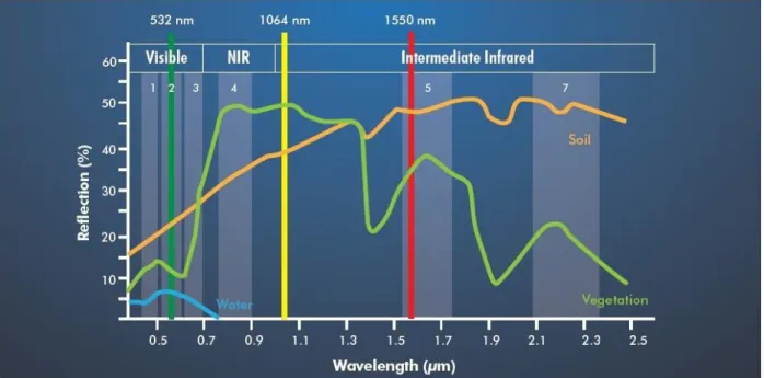
In addition to a typical ALS system mentioned in Chapter 1, a multispectral ALS system is capable of gathering discrete and full-waveform data from several different active imaging channels of different wavelengths, which may provide a better mapping ability of complicated environments. The first commercial multispectral airborne active imaging LIDAR sensor in the world is the Teledyne Optech Titan multispectral ALS system, which contains three active imaging channels of different wavelengths: 1550 nm (shortwave infrared, SWIR), 1064 nm (near infrared, NIR), and 532 nm (green, G), respectively. The three channels generate laser pulses with separate forward angles to produce independent scan lines. As shown in Figure 2.1, green vegetation is strongly reflective in the NIR spectrum, and slightly reflective in the visible G spectrum. Soil tends to reflect most at the SWIR band but lowest at the green band. Electromagnetic waves are mostly absorbed at the water surface in the NIR and SWIR spectrum. Thus, the three scanning frequencies provided by the Teledyne Optech Titan make it possible to acquire various spectral responses of different materials and to obtain diverse information about the surface of the Earth (Bakuła, 2015). Detailed specifications of the Teledyne Optech Titan are listed in Table 2.1. This section introduces the multispectral ALS System in terms of its components, direct geo-referencing theory, basic principles, and multi-wavelength intensity maps.

(20)

Figure 2.1 Titan laser channels with spectral signatures for selected objects (Teledyne Optech Titan, 2015)

Table 2.1 Specifications of Titan

Parameter Specification

Wavelengths Channel 1: 1550 nm (shortwave infrared, SWIR) Channel 2: 1064 nm (near infrared, NIR) Channel 3: 532 nm (green, G)

Forward Angles Channel 1: 3.5° Channel 2: 0° Channel 3: 7°

Pulse repetition frequency (PRF) Programmable; 50 - 300 kHz per channel; 900 kHz in total Scan Frequency Programmable; 0 - 210 Hz

Point density Bathymetric: >15 pts/m2 Topographic: >45 pts/m2

Accuracy Horizontal: 1/7, 500 × altitude,1 σ Vertical: < 5 - 10 cm, 1σ

Laser range precision 5 < 0.008 m; 1 σ

2.1.1 Components of a Multispectral ALS System

The components of the Teledyne Optech Titan multispectral ALS system are shown in Figure 2.2. A flight management system, an operator laptop, a digital camera, a laser scanner assembly, a

(21)

Global Navigation Satellite System (GNSS), an Inertial Measurement Unit (IMU), and a control and data recording unit are essential parts of a Multispectral ALS system.

Figure 2.2 Optech Titan system (Teledyne Optech Titan, 2015) (1) Flight Management System

A flight management system provides pre-planned flight lines, real-time point display, and real-time survey conditions, which guarantee uncomplicated operation and consistent point distribution. Titan offers a Teledyne Optech’s comprehensive flight management system to operators.

(2) Operator Laptop

The operator laptop builds communications between operators and the control and data recording unit in order to allow operators to set up parameters. Operators can control a multispectral ALS system and monitor the system performance using an operator laptop.

(3) Digital Camera

A digital camera is often implemented in the fuselage exposed to the ground to provide ancillary information via taking colour images or videos of the study area concurrently with laser scanning. For example, the true-colour information of these images or videos can be used to colorize the points collected by laser scanners to achieve a better visualization. The Titan system also provides a digital camera. However, the digital photos collected by the Titan system are not

(22)

available for this study. (4) Laser Scanner

The laser scanner assembly releases continuous laser beams towards the target to capture surfaces of objects and measure the distances to objects. A laser scanner in a multispectral ALS system is set to work in a 2D planar-scanning mode; the third dimension of the collected 2D data can be achieved by moving the aircraft. Different parameters of laser scanners such as field-of-view, range, and scan frequency lead to different quality of collected data. For example, the Titan can achieve a point density of 25 points/m2_{with a flying height of 1000 m, Pulse repetition}

frequency (PRF) of 900 kHz, field of view (FOV) of 30, and a cruising speed of 60 m/s. (5) GNSS

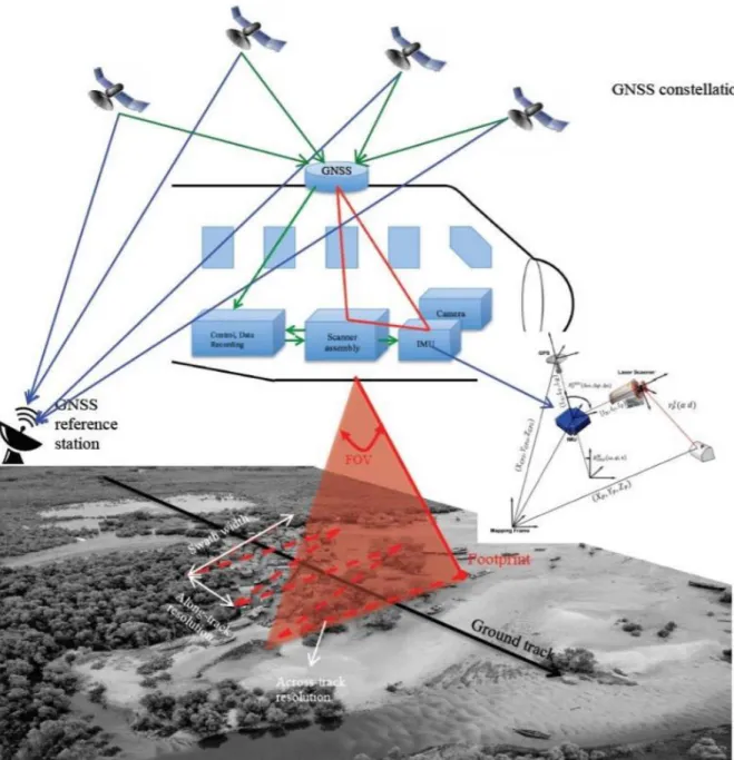
A GNSS, which is fixed at the top of the aircraft, is the fundamental module of a positioning system. It has the ability to provide centimetre accuracy positions. Integrated with an IMU (see Figure 2.3), a GNSS can provide precise orientation measurement and position information for an airborne sensor. The multispectral ALS system implements these two navigation sensors rather than using one of them alone to exploit the complementary nature of these sensors. In this integrated navigation system, GNSS offers three prime surveys: position, time, and velocity that includes speed and direction. Though GNSS receivers can deliver exceedingly precise position measurements in an open environment, it is practically impossible to receive the signal during a complete survey due to multipath effects and the GNSS outage periods. This limitation can be surmounted by combining the GNSS and IMU data streams.

(6) IMU

An IMU sensor, which comprises a microcomputer unit and a set of gyroscopes and accelerometers, can calculate the updated positions and velocities for an initial position and attitude provided by GNSS. Acceleration information provided by IMU facilitates the interpolation of the aircraft position along the GNSS trajectory. Rotation rates recorded by IMU are utilized to determine the orientation of the aircraft. The velocities, positions, and orientations calculation of IMU is autonomous and safe from blockage since no external information is required. Attitude information such as heading, pitch, and roll can be provided by IMU without the assistance of satellite signals; nevertheless, the accuracy of the orientation and position degrades with the time. Thus, the IMU sensor is inappropriate to be used alone but can complement a GNSS; GNSS offers updated location information to the IMU while the IMU provides complementary position

(23)

information when the GNSS satellite conditions are poor.

Figure 2.3 Cooperation principle of GNSS and IMU (Chen et al, 2018) (7) Control and Data Recording Unit

This unit controls the whole system and records ranging and positioning data collected by the laser scanner, GNSS, and IMU.

2.1.2 Direct Geo-referencing

Direct geo-referencing is the determination of time-variable position and orientation parameters for a multispectral ALS system, which produces corresponding coordinate information

(24)

for each recorded point. The position (p(t)) of a recorded point at a time can be calculated using the following well-defined geo-referencing formula:

𝑝(𝑡) = 𝑝_𝑁(𝑡) + 𝑅_𝑁(𝑡) ∗ 𝑅_𝑆(𝑡) ∗ 𝑟_𝐿(𝑡) (2.1) where 𝑝𝑁(𝑡), in a 3D Cartesian geographic coordinate system, is the location of the scanner at time

t; the rotation matrix 𝑅𝑁(𝑡) describes the orientation of the laser channel; the rotation matrix 𝑅𝑆(𝑡)

defines the orientation of the scanning mechanism and process; and 𝑟𝐿(𝑡) refers to the range

measured by the laser scanner at time t (Hebel and Stilla, 2012).

2.1.3 Basic Principles of Multispectral ALS System

The laser scanner mentioned above measures the range of its surroundings. There are two primary methods utilized for range measurements in current ALS systems: time-of-flight (TOF) and phase shift (Vosselman and Maas, 2010). A TOF scanner emits a short laser pulse to the object, and records the time difference between the sent and received pulses to measure the range according to the propagation velocity of light in a medium (Vosselman and Maas, 2010). The following formula can be used to calculate the range:

R = 𝑐

𝑛∗ 𝑡

2 (2.2)

where c is the speed of light; t is the return time difference; and n is the refractive index of the medium (n≈1.00025 in air) (Vosselman and Maas, 2010). The TOF range measurement approach is applied in the Titan.

Phase-based range measurement in continuous wave modulation is regarded as an indirect form of TOF-based range measurement (Guan et. al., 2016). Phase-based laser scanners record the phase difference between the sent and received backscattered signals of an amplitude modulated continuous wave to measure the range (Puente, 2013). Commonly, the phase-based mode has higher accuracy ranging from sub-millimetre to sub-centimetre and has extremely high data rates, but shorter measuring ranges (Vosselman and Maas, 2010). The following formula can be used to calculate the range for phase-based ranging systems:

R = 𝜑 2𝜋∗ 𝜆 2+ 𝜆 2∗ n (2.3)

where φ is the phase shift; λ is the modulation wavelength; and n is the unknown number of full wavelengths between the sensor system and the reflecting object (Puente, 2013).

The swath width sw of a laser scanner can be specified by the following formula: 𝑠𝑤 = 2ℎ ∗ tan (𝜃

(25)

where θ represents the scan angle and h is the height of the aircraft above ground. The scan angle of Titan is programmable between 0°and 60°. This is a nominal formula for nadir scanning over flat terrain.

The width of a laser beam varies with the distance from the laser scanner. Assuming the spot shape (i.e. footprint) to be a circle, the diameter Ds of the illuminated footprint on the ground can be described by:

𝐷𝑠 = 2ℎ ∗ tan ( 𝛾

2) (2.5)

where h is the height of the aircraft above ground and γ is the beam divergence. In Titan, the beam divergence of both Channel 1 and Channel 2 is about 0.35 mrad; and this parameter of Channel 3 is around 0.7 mrad. Thus, the footprint (i.e. diameter on the ground) of a laser beam in Channel 1 and Channel 2 is about 16 cm, and about 32 cm in Channel 3 for a 457m flying height. In addition, the irradiance of a laser beam decreases progressively away from the centre of the beam. In Titan, the irradiance declines to 1/e times of the total irradiance.

2.1.4 Multi-wavelength Intensity Maps

For each measured point, an ALS system also records the strength of the backscattered echo, typically referred to as intensity, besides the spatial information based on TOF measurements. Recorded intensity not only is related with target’s reflectance at the given laser wavelength, but also depends on several other factors, such as wetness and roughness of the target surface,

environmental effects, data acquisition geometry parameters, and instruments (Bakuła, 2015;

Ahokas et. al., 2016). Fortunately, intensity calibration and normalization can be applied to reduce the effects of other factors and therefore improve the quality of intensity information (Yan et. al., 2012; Kashani et. al., 2015).

However, since common LiDAR only measures the backscatter at a single and narrow laser wavelength band, the utility of its intensity information has been essentially limited. To break this limitation, a multispectral ALS system provides the intensity information at multiple laser wavelength. For example, Titan can record the backscatter at three wavelengths (i.e. bands): SWIR, NIR, and G. In order to analyse and utilize the intensity information collected at different bands more easily, for each band, the intensity information of 3D point cloud is often converted into a 2D raster imagery which allocates the intensity as the cell value (e.g. Matikainen et. al.,

(26)

2016; Bakuła et. al., 2016). The selection of the cell size usually relies on the point density of a dataset.

2.2 LC Classification for Multispectral ALS Datasets

Since the multispectral ALS technique is still an emerging technology, there are limited studies exploring its feasibility for the LC classification. All studies which tested the accuracy of LC classification using different multispectral ALS datasets are summarized in Table 2.2. Details of these studies are analysed and compared in the following sections.

Table 2.2 Studies Related to Multispectral ALS Data Classification

Authors Type Main Algorithm Classes Overall

Accuracy

Kappa Bakuła et. al., (2016) Raster-based Maximum Likelihood 6 90.9% 0.88 Fernandez-Diaz et.

al., (2016)

Raster-based Maximum Likelihood 5 90.2% 0.87 Morsy et. al., (2017a) Raster-based Maximum Likelihood 4 89.9% 0.86 Teo and Wu, (2017) Object-based Support Vector Machine 5 96% 0.95 Matikainen et. al.

(2016; 2017a; 2017b)

Object-based Random Forest 6 95.9 0.95

Zou et al. (2016) Object-based Decision Tree 9 91.6% 0.89 Wichmann et al.

(2015)

Point-based Progressive TIN Densification; RANSAC-based Segmentation

5 99% N/A

Morsy et. al., (2017a) Point-based Skewness Balancing;

Jenks natural breaks optimization

4 92.7% 0.90

Morsy et. al., (2017b) Point-based Skewness Balancing; Gaussian Decomposition; Maximum Likelihood

4 95.1% 0.93

2.2.1 Potential of Multispectral ALS technique in LC classification

Even though just a few related studies have been published, the potential of using multispectral ALS technique to map the surface of the Earth has been illustrated.

On one hand, it has been proven that multispectral ALS techniques are superior to traditional multispectral optical techniques for LC classification. To explore the superiority of multispectral ALS data compared to typical multispectral optical images for LC classification, Bakuła et. al. (2016) selected different inputs of classification: only spectral information recorded on the laser reflectance intensity images, spectral information with elevation data derived from 3D coordinate

(27)

of laser points, and spectral information with elevation and textural data derived from granulometric analysis of the point cloud. The result indicates the utilization of elevation information could significantly improve the classification output, especially in the situation that separating objects with distinctive height was required (Bakuła et. al., 2016). Similarly, after comparing classification results when using only spectral information from the three Titan channels with classification results from a combination of the structural images and the intensity images, both Fernandez-Diaz et al. (2016) and Morsy et al. (2017) found that the addition of structural images derived from multispectral ALS data increased the classification accuracy by more than 15%. Furthermore, Teo and Wu (2017) proposed that using a combination of spectral and geometrical features extracted from multispectral ALS point clouds improved the “road” class extraction in urban area by 15.2% when compared to using only spectral features. In addition, compared to passive aerial images, the intensity images have interesting advantages such as a lack of shadows. Thus, it can be concluded that the multispectral ALS point clouds have higher potential for LC classification than typical multispectral optical images

On the other hand, multispectral ALS techniques have been shown to attain better accuracies of LC classification compared to typical single-wavelength ALS techniques. Teo and Wu (2017) concluded the improvement of classification completeness and overall accuracy from single-wavelength to multi-single-wavelength ALS technique ranged from 1.7% to 42.3% and from 4% to 14%, respectively. The most significant accuracy improvement brought by the multispectral information occurred in the “Soil” class with an improvement of 35.8% (Teo & Wu, 2017). Similarly, in a comparative study, Matikainen et. al. (2017a) stated that using intensity information of only Channel 1 to replace intensity information provided by all three channels resulted in a marked reduction of classification accuracy.

Since multispectral ALS techniques have such a high potential for LC mapping, it is necessary to seek optimal classification methods in order to take full advantages of the dataset.

2.2.2 Classification Methods Used for Multispectral ALS Datasets

It is well known that the accuracy of classification highly relies on the classification algorithms and the information provided by the input; more reliable classification algorithms and more useful input information lead to better classification results. Since multispectral ALS datasets can produce similar data product derived from both typical multispectral optical images (e.g. multi-wavelength intensity images) and ALS point clouds (e.g. height model), most classification algorithms

(28)

designed for either remote sensing imagery or ALS point clouds can also be used for multispectral ALS datasets. The problem is how to extract useful information from multispectral ALS point clouds and how to input the appropriate information with an acceptable format into appropriate classification algorithms.

To standardize an acceptable format of multispectral-ALS-derived data products for classification algorithms, a specific classification model type should be identified for each LC classification experiment. Generally, classification models can be categorized into two types: raster-based classification models and object-based classification model. The former classifies the Earth’s surface based on the information in each raster cell; while the latter is based on information related to each object, which is a set of similar pixels related to a measure of spectral properties, shape, size, texture, context, and relationship with neighbours as well as super-, and sub-pixels (Weng, 2012). Object-based models usually involve two steps: data segmentation to generate objects and classification of the segmented objects. With regard to LiDAR point clouds, there is a third type of classification model, which classifies the Earth’s surface based on points. Different classification model types may lead to different reorganization procedures for points such as rasterization and, therefore, result in different information loss. Furthermore, the type of classification model may limit the use of information extracted from the multispectral ALS point clouds and the selection of classification algorithms. The model types, algorithms, and inputs together affect the accuracy of a LC classification.

(1) Maximum Likelihood Classification (MLC)

One of the most widely used classification algorithms is the MLC algorithm, which assigns cells a LC class based on the measure of the highest likelihood. The MLC algorithm is generally implemented to classify LC based on the information in each raster cell. Bakuła et. al. (2016) presented an experiment using the raster-based MLC to classify a multispectral ALS point cloud into six classes, achieving an overall accuracy of 91% in the best test. This best attempt integrated multi-wavelength intensity images, elevation data, and textural data as the input. In this attempt, raster cells that belonged to water, trees, and buildings were classified accurately; however, cells which belonged to the classes "sand and gravel" and "asphalt and concrete" were misclassified because it was difficult for the MLC algorithm to distinguish two similar classes from each other when there was a shortage of distinctive features (Bakuła et. al. 2016). The raster-based MLC method was also applied by Morsy et al. (2017). Integrating the three raster intensity images with

(29)

the DSM raster image, this research obtained an overall accuracy of 89.9%. Similarly, Fernandez-Diaz et al. (2016) implemented a supervised raster-based MLC to categorize a multispectral ALS dataset into five LC classes with best overall accuracy of 90.2%. The best overall accuracy was obtained when structural images and only two intensity images derived from Channel 2 and Channel 3 were used. Addition of an intensity image of Channel 1 decreased the classification accuracy unexpectedly. The authors (Fernandez-Diaz et al., 2016) explained that spectral information provided by Channel 1 increased the within-class variance of the commercial buildings significantly, and therefore increased the correlation between commercial and residential building classes, leading to misclassification of the two classes. To conclude, although all of the above studies used the same raster-based MLC method and acquired satisfactory results, classification accuracy of different classes varied with different inputs. Furthermore, as a parametric classifier, the maximum likelihood classifier assumes that a training sample is normally distributed, which is often not the case. This incorrect assumption can introduce errors when classifying urban landscapes. Therefore, non-parametric methods are preferred for urban LC classification.

(2) SVM and Random Forest (RF)

Among a number of non-parametric methods, SVM and RF have been proven to be effective for LC classification.

SVM applies optimization algorithms to determine the location of ideal boundaries that can most effectively distinguish between classes (Huang et al., 2002). Although SVM was initially developed for handling binary class problems, it has been extended for multi-class problems (Pal and Mather 2005). In principle, the SVM technique aims to reduce the misclassification errors by locating a hyperplane which splits the dataset into a number of discrete classes (Luque et al, 2013). An object-based SVM classification method was tested by Teo and Wu (2017) to categorize multispectral ALS points into 5 classes. The points were firstly segmented to objects according to heterogeneity index, which combined both attribute and shape factors. Then, a supervised SVM was applied to classify the objects, attaining an overall accuracy of 96%. Although the overall accuracy was remarkable, SVM classification still had a major limitation related to the selection of the kernel function and the setting of proper parameter values since they were decided subjectively by the user; few studies have been conducted concerning the optimal choice of a kernel function and proper settings for corresponding parameters (Petropoulos et al, 2012).

(30)

The RF algorithm proposed by Breiman (2001) is based on the random selection of input training data. The RF method is a collection of Decision Trees. A decision tree, which is the predictive model that uses a set of binary rules as nodes to acquire a best solution, can also be used as a LC classification algorithm. An object-based decision tree model was implemented with the multispectral ALS data by Zou et al. (2016) to accomplish a 9-class LC classification. In this study, they produced a pseudo normalized difference vegetation index to improve identification of vegetation classes, reaching an overall accuracy of 91.6%. However, the decision tree algorithm tends to overfit training data, especially when a tree is particularly deep. Random forests mitigate this problem well without substantially increasing errors. To constitute a RF, firstly decision trees are formed by randomly sampling a subset (usually 2/3) of the training data and variables with constant replacement. For each tree, a set of user-defined input features for each subset of training sample are selected to determine the decision criteria at the node. Then, the best split at each node is determined by sampling this subset of features via creating a binary rule (Breiman, 2001). Since this algorithm does not necessitate separate feature selection or feature values normalization, it is appropriate for classifying data with a large number of features (Matikainen et. al., 2017a). Matikainen et al. published several articles (2016; 2017a; 2017b) to discuss the performance of an object-based RF LC classification method. They indicated that this method could achieve an outstanding classification result using multispectral ALS datasets, especially in terms of “Building”, “Tree”, and “Asphalt” classes (accuracy of “Building” = 100%, “Tree” = 97.9%, and “Asphalt” = 97.4%). However, this method led to low completeness and correctness values for “Gravel” class as the number of gravel points was relatively small and the in-class variation was comparatively large (Matikainen et al., 2017a). Furthermore, the large number of trees in this method may make the classification process slow, especially when applied to a large dataset such as a dense multispectral ALS point cloud in a large area.

In the context of classic machine learning algorithms, both SVM and RF provide precise and reliable classification results for multispectral ALS data. Nevertheless, both of them require manually designed features which significantly impact the classification accuracy. This characteristic of classic machine learning algorithms makes them highly user-dependent.

(3) Other Multi-phase Methods

To reach higher classification results using multispectral ALS datasets, point-based multi-algorithm and multi-phase methods were generated. Wichmann et al. (2015) firstly applied a

(31)

hybrid approach of progressive TIN densification to separate points that belonged to “Ground” class; and then, they combined RANSAC-based point cloud segmentation algorithm and other point cloud features such as eigenvalue-based omnivariance to classify the remaining non-ground points into building and vegetation classes. Even through this automatic multi-phase method achieved an extremely high overall accuracy of about 99%, it did not classify ground points into sub-classes, which made this LC classification not detailed enough. The point-based multi-algorithm and multi-phase methods were also usedin two LC classification studies (Morsy et al. 2017a; 2017b). In the first research, Morsy et al. (2017a) initially divided points into non-ground points and ground points based on the skewness balancing algorithm; and then, they applied the Jenks natural breaks optimization method to define threshold of NDVI values and cluster both non-ground points and ground points into detailed classes. The best overall accuracy obtained by this point-based method was 92.7%. To achieve a better classification results, Morsy et al. (2017b) designed another point-based multi-algorithm method for the same multispectral ALS dataset. In this new method, instead of the Jenks natural breaks optimization algorithm, the maximum likelihood algorithm was used based on Gaussian components decomposed by the Gaussian decomposition algorithm to cluster points into detailed classes. This new method obtained an overall accuracy of 95.1%. Although the multi-algorithm and multi-phase methods achieved relatively high accuracy, they were usually designed according to features of a particular multispectral ALS point cloud. The classification accuracy of these methods would significantly vary significantly with the data features such as the type, content, and distribution of LC, which rendered them inappropriate for widespread application.

To conclude, none of the existing classification methods represents an optimal method for classifying multispectral ALS data; most of these methods have serious weaknesses and cannot achieve accuracies higher than 96% in terms of multispectral ALS data classification. With an increasing demand for extremely high accuracy of LC classification, new classification methods should be proposed for multispectral ALS datasets that have high potential on LC mapping.

2.3 Deep learning

Rewarded as one of the ten breakthrough technologies of 2013 by Massachusetts Institute of Technology (MIT Technology Review, 2013), deep learning has been widely applied in the fields of artificial intelligence because of the notably reduced cost of computing hardware, the remarkably improved chip processing capabilities, and the significant developments of the

(32)

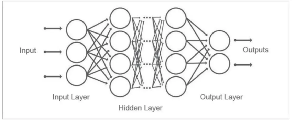
learning algorithms (Deng, 2014). The theory of deep learning builds on neural networks. A standard neural network is consists of numerous linked processors named neurons; each neuron can be activated by either an input environment or weighted connections from previously active neurons (Schmidhuber, 2015). Formed by a mass of neurons with more than two hidden layers (Figure 2.4), deep learning algorithms explore feature representations from data by themselves to learn high-level abstractions in data using hierarchical architectures (Guo et. al., 2016). More specifically, each neuron represents an input value called activation in the input layer and a function in the hidden layer. Each neuron in a hidden layer receives the activations provided by the prior layer, operates the activations based on the function and the given weights, and determines the activations that will be transferred to the next layer. To limit the activations within a specific range, before transferring the activations to the next layer, activation functions such as Sigmoid function and the rectified linear unit (ReLU) function are frequently applied to taper the activations into a specific range. After the last hidden layer yields activations to the output layer, a cost function is implemented to calculate the cost of the method. The aim of the learning process is to find optimal weights which make the neural network show a desired performance by minimizing the cost.

Figure 2.4 Structure of Standard Deep Neural Network

To allow readers to better understand deep learning and its application in LC classification, this section introduces deep learning through explaining the relationship between deep learning and machine learning, categorizing common deep learning algorithms into four types, and summarizing representative studies that classify remote sensing data using deep learning algorithms.

(33)

2.3.1 Relationship between Machine Learning and Deep Learning

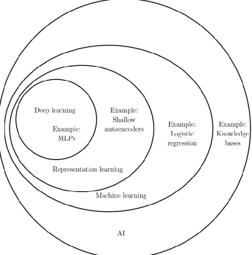
Generally, deep learning is a subfield of representation learning that is a subfield of machine learning. Figure 2.5 describes the relationship among them.

Figure 2.5 the Relationship among Deep Learning, Machine Learning, Representation Learning, and Artificial Intelligence (Goodfellow et al., 2016)

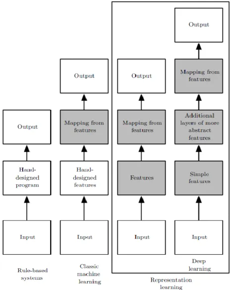
Deep learning also can be considered as a product of advance and evolution of classic machine learning (see Figure 2.6). Machine learning has the ability to acquire knowledge by extracting patterns from raw data, which allows computers to have the capability of handling problems that involve knowledge of the real world and to make decisions based on human-defined representation of data (Goodfellow et. al., 2016). Thus, for each machine learning algorithm, an appropriate set of features needs to be extracted and provided by designers. The human-defined representation highly impacts the performance of machine learning methods; the optimal set of features will lead to the best result of a machine learning algorithm. Nevertheless, in most instances, it is challenging to determine what features should be extracted. To solve this problem, representation learning has

(34)

been proposed. Representation learning utilizes the ability of machine learning to “discover not only the mapping from representation to output but also the representation itself” (Goodfellow et. al., 2016). The computer-designed representations of representation learning usually lead to significantly better performance than hand-designed representations. A primary target of representation learning is to extract the factors of variation that can explain the data. However, it is also challenging to extract such high-level abstract features from raw data. Thus, deep learning is raised to solve this crucial difficulty of representation learning via introducing simpler representations that can be used to build complex representations (Goodfellow et. al., 2016). It decomposes the desired complex mapping to multiple simple mappings described by multiple different layers of the model.

Figure 2.6 the Relationship among Deep Learning, Machine Learning, Representation Learning, and Rule-based Systems (Goodfellow et al., 2016)

(35)

2.3.2 Deep Learning Algorithms

Commonly, deep learning algorithms can be divided into four groups based on the elementary method that they apply (Figure 2.7): auto-encoder, Restricted Boltzmann Machine (RBM), sparse coding, and Convolutional Neural Networks (CNN).

Figure 2.7 Category and Representative Examples of Deep Learning Algorithms

The auto-encoder is often implemented for learning efficient encodings through reconstructing its own inputs rather than predicting a target value for the provided input (Liou et. al., 2014). A typical auto-encoder contains an encoder as well as a decoder to accomplish the reconstruction of inputs. A deep auto-encoder is formed by a series of typical auto-encoders with deterministic network architectures, in which the code learnt from the previous auto-encoder is transferred to the next encoder. Trained with variants of back-propagation, the deep encoder can efficiently obtain more discriminative and characteristic features than the typical auto-encoder (Zhang et. al., 2014). However, deep auto-auto-encoder sometimes can be ineffective especially when first few layers of this model yield errors and deliver them to posterior layers (Guo et. al., 2016).

Different from auto-encoders, which have deterministic network architectures, a RBM is a generative stochastic directionless graphical model designed by Hinton (1986). A classic RBM has a visible layer and a hidden layer; there is no connection within the hidden layer or the input layer (Zhu et. al., 2017). Although the feature representation ability of a single RBM is limited,

(36)

efficient deep models such as Deep Belief Networks (DBN) can be composed using RBMs as learning modules. A DBN is a probabilistic generative model applying a greedy learning approach. Nonetheless, as training a DBN involves the training of numerous RBMs, the implementation of the DBN model is computationally costly (Bengio et. al., 2013).

The sparse coding aims to describe the input data through learning a series of elementary functions (Olshausen and Field, 1997). This model has various benefits. Firstly, since the sparse coding utilizes multiple bases, it can positively restructure the descriptor and establish the relationships between similar descriptors identified by sharing bases. Also, noticeable characteristics of the data can be well described due to the sparsity of the sparse coding. Furthermore, data with sparse features can be more linearly separated.

The CNN, the most famous and commonly used deep learning method especially in the field of computer vision, is composed by convolutional layers, pooling layers, and fully connected layers. The CNN has a hierarchical architecture where convolutional layers alternate with pooling layers followed by fully connected layers. The convolutional layer is the main calculating part of a CNN, utilizing numerous kernels to convolve both the input image and the intermediate feature maps to produce multiple feature maps (Guo et. al., 2016). The convolution operation of CNN benefits deep learning process considerably especially in computer vision domains. It reduces the number of parameters due to the weight sharing mechanism, improves the understanding of correlations among neighbouring pixels, and does not change the location of the object (Zeiler, 2013). The pooling layer can be simply regarded to a down-sampling process which combines the outputs of neuron clusters at one layer into a single neuron in the next layer (Ciresan et. al., 2011). To gradually diminish the spatial size of the representation, decrease the number of parameters and calculation, and consequently control overfitting, a pooling layer is usually inserted in-between successive convolutional layers. The fully-connected layer transforms the 2D feature maps into a one-dimensional (1D) feature vector which is similar to a layer in the traditional neural network with about 90% of the parameters in the CNN (Guo et. al., 2016). The vector can be considered as a feature vector for further processing (Girshick et. al., 2014). The training process of CNN consists of forward steps and backward steps. The forward step aims to generate feature maps in each layer based on the current parameters such as weights and bias. The prediction output of this forward process and the given ground truth labels are utilized to calculate the loss cost. Then, a backward step is applied to calculate the gradient of each parameter. These gradients are

(37)

used to update all the parameters such as weights and bias in each layer. With these updated parameters the system can proceed to the next forward calculation. The circulation can be stopped when the loss cost of the model or the number of iterations of the forward and backward stages reaches a specified threshold.

Figure 2.8, established by Guo et. al. (2016), summarized the benefits and drawbacks in terms of various properties. To be more specific, ׳Generalization׳ indicates whether the method has fine performance in various media and applications. ‘Real-time’ emphasizes the efficiency of the approach. ‘Invariance’ evaluates if the method has robustness in transformation such as scale, rotation, and translation (Guo et. al., 2016). In conclusion, the CNN performs best in automatic feature learning; the auto-encoder and the sparse coding are more efficient in training especially when the training datasets are small; the sparse coding is more suitable for biological studies and more invariant towards transformation.

Figure 2.8 Comparisons among Four Categories of Deep Learning Algorithms.

2.3.3 Deep Learning in LC Classification

Since deep learning has been verified to be a highly successful tool that sometimes its learning ability even exceeds humans’ (e.g. AlphaGo; Chen, 2016), it becomes the model of choice in many fields including remote sensing. As an evolution version of classic machine learning, deep learning

(38)

has been applied in different kinds of datasets for LC classification. To better understand how deep learning can improve LC classifications and which type of deep learning algorithms performs best for LC classifications, studies that apply deep learning to classify LC types for other remote-sensing data are referred to as there is no research has studied the feasibility of using deep learning to classify LC types for multispectral ALS data.

(1) High-Resolution (HR) Remote Sensing images

In recent years, HR remote sensing images especially very-high-resolution (VHR) images collected from satellites, planes, and unmanned aerial vehicles (UAV) have been widely used for LC classifications. In terms of the HR and VHR images, it has been proven than deep learning methods can achieve remarkable accuracies for LC classification.

Zhang et al. (2017a) proposed two object-based deep learning classification methods involving stacked auto-encoders (SAE) and stacked de-noising auto-encoders (SDAE), respectively. In this study, all the spectral, spatial, and texture features of each object segmented by graph-based minimal-spanning-tree segmentation algorithm were put into either SAE or SDAE network to accomplish classification of the objects (Zhang et al., 2017a). According to the research, the highest accuracy of both SAE-based method and SDAE-based method reached 97% when classifying the VHR images into five classes, which was about 6% higher than the overall accuracy of SVM (Zhang et al., 2017a). Furthermore, according to experiments completed by Papadomanolaki et al. (2016), deep CNN models such as AlexNet and VGG networks achieved better results of LC classification than other deep learning models including SDAE and DBN. For VHR images collected by SAT-4, both AlexNet and VGG networks reached an overall classification accuracy of 99.9%, while the overall accuracy of SDAE and DBN was 80.0% and 81.8%, respectively. Furthermore, Romero et al. (2016) stated that CNN usually performed better in LC classification for VHR images with more training samples and more hidden layers. (2) Hyperspectral Images

The hundreds of narrow spectral bands provided by hyperspectral images facilitate the identification of LC type of each pixel via spectroscopic analysis. Since the hyperspectral imaging procedure is inherently nonlinear (Ghamisi et al., 2016) and deep learning architectures are normally more robust towards the nonlinear processing, the fact that deep learning networks can benefit LC classification of hyperspectral images has been verified recently.

(39)

introducing deep learning method into hyperspectral data classification was completed by Chen et al. (2014). They designed a deep learning-based framework which integrated SAE and logistic regression (LR) together to classify hyperspectral images. The authors indicated that the SAE-extracted features were more helpful for LC classification, compared to other traditional methods of feature extraction such as principle component analysis and nonnegative matrix factorization. Since it was a supervised classification method, data labelling was needed, which increased the difficulty of extensive use. To avoid data labelling, Tao et al. (2015) proposed an unsupervised classification method that used the stacked sparse auto-encoder (SSAE) to learn features from unlabelled data. Their experiments demonstrated that features learned by SSAE were more robust for hyperspectral data classification compared to the traditional handcraft features. Both of the auto-encoder-based methods achieved a good overall accuracy of above 97% for hyperspectral data classification.

RBM was also applied in hyperspectral data classification. Chen et al. (2015) presented a new hyperspectral image classification framework based on DBN. Diminishing the feature dimension and presenting a good reconstruction, DBN was an effective method for hyperspectral data classification. Using the DBN-based method, the overall accuracy of hyperspectral image classification reached 99%.

Moreover, CNNs were widely used for hyperspectral data classification. Since the availability of labelled hyperspectral data, supervised CNN has been well studied. Hu et al. (2015) designed a simple 1D CNN with only one convolutional layer, one max-pooling layer, and one fully connected layer to directly classify hyperspectral images. Their experimental results validated that the CNN-based method could achieve higher classification accuracy than traditional methods like SVM. Makantasis et al. (2015) proposed a 2D CNN for hyperspectral data classification which also performed as well as the 1D CNN. To compare the 1D and 2D CNN, Kussul et al. (2017) applied them separately to classify the same dataset. They concluded that the 2D CNN was superior to the 1D CNN in terms of overall accuracy; however, the 2D CNN was more likely to misclassify small objects and lead to overfitting. To solve this problem, Ghamisi et al. (2016) suggested a self-improving 2D CNN-based classification model to iteratively select the most informative bands based on the fractional-order Darwinian particle swarm optimization algorithm. This model was also useful to solve the so-called curse of dimensionality. The challenges of dimensionality could also be avoided by an end-to-end deep learning network proposed by Santara et al. (2017) by