Comparing patterns of default among prime and
subprime mortgages
Gene Amromin and Anna L. Paulson
Gene Amromin is a senior financial economist in the Financial Markets Group and Anna L. Paulson is a senior financial economist in the Economic Research Department at the Federal Reserve Bank of Chicago. The authors are grateful to Leslie McGranahan for very helpful feedback and to Edward Zhong and Arpit Gupta for excellent research assistance.
Introduction and summary
We have all heard a lot in recent months about the soaring number of defaults among subprime mortgage borrowers; and while concern over this segment of the mortgage market is certainly justified, subprime mortgages account for only about one-quarter of the total outstanding home mortgage debt in the United States. The remaining 75 percent is in prime loans. Unlike subprime loans, prime loans are made to bor-rowers with good credit, who fully document their in-come and make traditional down payments. Default rates on prime loans are increasing rapidly, although they remain significantly lower than those on subprime loans. For example, among prime loans made in 2005, 2.2 percent were 60 days or more overdue 12 months after the loan was made (our definition of default). For loans made in 2006, this percentage nearly doubled to 4.2 percent, and for loans made in 2007, it rose by an-other 20 percent, reaching 4.8 percent. By comparison, the percentage of subprime loans that had defaulted after 12 months was 14.6 percent for loans made in 2005, 20.5 percent for loans made in 2006, and 21.9 percent for loans made in 2007. To put these figures in perspec-tive, among loans originated in 2002 and 2003, the share of prime mortgages that defaulted within 12 months ranged from 1.4 percent to 2.2 percent and the share of defaulting subprime mortgages was less than 7 percent.1 How do we account for these historically high default rates? How have recent trends in home prices affected mortgage markets? Could contemporary observers have forecasted these high default rates?
Figure 1, panel A summarizes default patterns for prime mortgages; panel B reports similar trends for subprime mortgages. Both use loan-level data from Lender Processing Services (LPS) Applied Analytics. Each line in this figure shows the cumulative default experience for loans originated in a given year as a
function of how many months it has been since the loan was made. Several patterns are worth noting. First, the performance of both prime and subprime mortgages has gotten substantially worse, with loans made in 2006 and 2007 defaulting at much higher rates. The default experience among prime loans made in 2004 and 2005 is very similar, but for subprime loans, default rates are higher for loans made in 2005 than in 2004. Default rates among subprime loans are, of course, much higher than default rates among prime loans. However, the deterioration in the performance of prime loans happened more rapidly than it did for subprime loans. For example, the percentage of prime loans that were 60 days or more overdue grew by 95 percent for loans made in 2006 compared with loans made in 2005. Among subprime loans it grew by a relatively modest 53 percent.
Home prices are likely to play an important role in households’ ability and desire to honor mortgage commitments. Figure 2 describes trends in home prices from 1987 through 2008 for the ten largest metropoli-tan statistical areas (MSAs). This figure illustrates the historically high rates of home price growth from 2002 through 2005, as well as the sharp reversal in home prices beginning in 2006. One of the things we con-sider in this article is whether prime and subprime loans responded similarly to these home price dynamics.
Although the delinquency rate among prime mortgages is high and rising fast, it is only about one-fifth the delinquency rate for subprime mortgages.
Unfortunately, however, this does not mean that total losses on prime mortgages will be just one-fifth the losses on subprime mortgages. The prime mortgage market is much larger than the subprime mortgage market, representing about 75 percent of all outstand-ing mortgages (International Monetary Fund, 2008),
or a total of $8.3 trillion.2 Taking the third quarter of
2008 as the starting point, we estimate that total loss-es from prime loan defaults will be in the neighbor-hood of $133 billion and that total losses from
subprime loan defaults will be about $364 billion.3
Losses on prime mortgages are also distributed very differently from losses on subprime mortgages. Most prime mortgages for amounts at or below $417,000 are guaranteed through the government-sponsored enterprises (GSEs), such as Fannie Mae and Freddie Mac.4 Losses on these mortgages that exceed
the ability of the GSEs to satisfy their obligations are ultimately borne by the taxpayer.5 In contrast, prime
mortgages for amounts greater than $417,000 (“jumbo” loans) and subprime mortgages were largely securi-tized privately, and absent government intervention, investors in asset-backed securities linked to those
4 FIguRE 1
Cumulative default rates for prime and subprime mortgages
A. Prime mortgages
percent
B. Subprime mortgages
percent
Note: Each year indicates the year of mortgage origination.
Source: Authors’ calculations based on data from Lender Processing Services (LPS) Applied Analytics.
1 2 3 4 5 6 7 8 9 10 11 12 13 14 15 16 17 18 19 20 21 22 23 24 0 2 4 6 8 10 12 1 2 3 4 5 6 7 8 9 10 11 12 13 14 15 16 17 18 19 20 21 22 23 24 0 5 10 15 20 25 30 35 40 2006 2005 2007 2004 2005 2007 2004 2006 months since mortgage origination
mortgages are the ones that are most exposed to de-clines in their value due to increasing defaults.
In this article, we make use of loan-level data on individual prime and subprime loans made between January 1, 2004, and December 31, 2007, to do three things: 1) analyze trends in loan and borrower charac-teristics and in the default experience for prime and sub-prime loans; 2) estimate empirical relationships between home price appreciation, loan and borrower characteris-tics, and the likelihood of default; and 3) examine whether using alternative assumptions about the behav-ior of home prices could have generated more accu-rate predictions of defaults. Throughout the analysis, we divide the loans into eight groups based on two characteristics: prime versus subprime and the “vin-tage,” the year in which the loan was made.
First, we describe trends in loan and borrower characteristics, as well as the default experience for prime and subprime loans for each year from 2004 through 2007. Next, we estimate empirical models of the likelihood that a loan will default in its first 12 months. This allows us to quantify which factors make default more or less likely and to examine how the sensitivity to default varies over time and across prime and subprime loans. Finally, we use these results to examine whether market participants could have forecasted default rates more accurately, that is, could have made predictions that were closer to actual default rates, by using alternative assumptions about the be-havior of home prices. This article draws on much of the very informative literature on the performance of
subprime loans, including, Bajari, Chu, and Park (2008); Chomsisengphet and Pennington-Cross (2006); Demyanyk and Van Hemert (2009); Dell’Ariccia, Igan, and Laeven (2008); DiMartino and Duca (2007); Foote et al. (2008); Gerardi, Shapiro, and Willen (2008); Gerardi et al. (2008); and Mian and Sufi (2009). By including prime loans in the analysis, our intention is to complement the existing literature on subprime loans.
By looking at prime and subprime loans side by side, we also hope to refine the possible explanations for the ongoing mortgage crisis. Both prime and sub-prime loans have seen rising defaults in recent years, as well as very similar patterns of defaults, with loans made in more recent years defaulting at higher rates. Because of these similarities, it seems reasonable to expect that a successful explanation of the subprime crisis—the focus of most research to date—should also account for the patterns of defaults we observe in prime mortgages.
We find that pessimistic forecasts of home price appreciation could have helped to generate predic-tions of subprime defaults that were closer to the ac-tual default experience for loans originated in 2006
and 2007.6 However, for prime loans this would not
have been enough. Contemporary observers would have also had to anticipate that default among prime loans would become much more sensitive to changes in home prices. Among prime loans originated in 2006 and 2007, defaults were much more correlated with changes in home prices than was the case for prime loans originated in 2004 and 2005. While this
FIguRE 2
Historical levels of home prices for top ten U.S. metropolitan statistical areas, 1987–2008
Source: Standard and Poor’s (S&P) and Fiserv Inc., S&P/Case-Shiller Home Price Indexes, seasonally adjusted Composite-10 Index (CSXR-SA).
index, Jan. 2000 = 100 0 50 100 150 200 250 1987 ’88 ’89 ’90 ’91 ’92 ’93 ’94 ’95 ’96 ’97 ’98 ’99 2000 ’01 ’02 ’03 ’04 ’05 ’06 ’07 ’08
pattern is straightforward to document now, it would have been difficult to anticipate at the time.
Loan and borrower characteristics
In this section, we discuss trends in loan and borrower characteristics, as well as the default experi-ence for prime and subprime loans for each year from 2004 through 2007.
Data
The loan-level data we use come from LPS Applied Analytics, which gathers data from a number of loan servicing companies.7 The most recent data
include information on 30 million loans, with smaller, but still very large, numbers of loans going back in time.
The data cover prime, subprime, and Alt-A loans,8
and include loans that are privately securitized, loans that are sold to the GSEs, and loans that banks hold on their balance sheets. Based on a comparison of the LPS and Home Mortgage Disclosure Act (HMDA) data, we estimate that the LPS data cover about 60 percent
of the prime market each year from 2004 through 2007.9
Coverage of the subprime market is somewhat small-er, but increases over time, going from just under 30 percent in 2004 to just under 50 percent in 2007.
The total number of loans originated in the LPS data in each year of the period we study ranges from a high of 6.2 million in 2005 to a low of 4.3 million
in 2007.10 The mortgage servicers reporting to LPS
Applied Analytics give each loan a grade of A, B, or C, based on the servicer’s assessment of whether the loan is prime or subprime. We label A loans as prime
loans and B and C loans as subprime loans.11 To make
the analysis tractable, we work with a 1 percent random sample of prime loans made between January 1, 2004, and December 31, 2007, for a total of 68,000 prime loans, and a 10 percent random sample of subprime loans made during the same time period, for a total of 62,000 subprime loans.
The LPS data include a wide array of variables that capture borrower and loan characteristics, as well as the outcome of the loan. The variables that we use in the analysis are defined in box 1. In terms of borrower characteristics, important variables include the debt-to-income ratio (DTI) of the borrower (available for a subset of loans) and the borrower’s creditworthiness, as
measured by his Fair Isaac Corporation (FICO) score.12
Some of the loan characteristics that we analyze include the loan amount at origination; whether the loan is a fixed-rate mortgage (FRM) or adjustable-rate mortgage (ARM); the ratio of the loan amount to the value of the home at origination (LTV); whether the loan was intended for home purchase or refinancing and, in case
of the latter, whether it involved equity extraction (a “cash-out refinance”); and whether the loan was sold to one of the GSEs, privately securitized, or held on the originating bank’s portfolio.
The outcome variable that we focus on is whether the loan becomes 60 days or more past due in the 12 months following origination. We focus on the first 12 months, rather than a longer period, so that loans made in 2007 can be analyzed the same way as earlier
loans, as our data are complete through the end of 2008.13
We augment the loan-level data with information on local economic trends and trends in local home prices. The economic variable we focus on is the local unem-ployment rate that comes from U.S. Bureau of Labor Statistics monthly MSA-level data. Monthly data on home prices are available by MSA from the Federal Housing Finance Agency (FHFA)—an independent federal agency that is the successor to the Office of Federal Housing Enterprise Oversight (OFHEO) and other government entities.14 We use the FHFA’s all transactions House Price Index (HPI) that is based on repeat sales information.
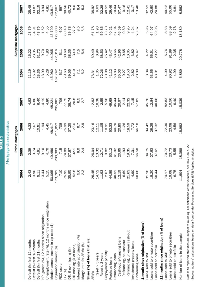
Trends in loan and borrower characteristics Many commentators (see, for example, Demyanyk and Van Hemert, 2009) have noted that subprime lending standards became more lax during the period we study, meaning that the typical borrower may have received less scrutiny over time that it became easier for borrowers to get loans overall, as well as to get larger loans. These trends have been particularly well documented for subprime loans, but there has been less analysis of prime loans. Table 1 summarizes mortgage characteristics for each year from 2004 through 2007 for prime and subprime mortgages. Consistent with prior work, we also document declining borrower quality over time in the subprime sector. For example, the average FICO score for sub-prime borrowers in 2004 was 617, but it had declined
to 597 by 2007.15 By contrast, when we look at prime
loans, the decline in lending standards is less obvious. The average FICO score among prime borrowers was 710 in 2004 and 706 in 2007, a decline of less than 1 percent.
Another potential indicator of the riskiness of a mortgage is the reason for taking out the loan: to buy a house or to refinance an existing mortgage. People who are buying a home include first-time home buyers who tend to be somewhat riskier, perhaps because they have stretched to accumulate the necessary funds to purchase a home or perhaps because they tend to be younger and have lower incomes. While we do not have data on whether loans for home purchase go to
BOX 1 Definitions of variables
Variable Description
Default (%) first 12 months Share of loans that are 60 days or more delinquent, in foreclosure, or real estate owned within 12 months of origination
Default (%) first 18 months Share of loans that are 60 days or more delinquent, in foreclosure, or real estate owned within 18 months of origination
Default (%) first 21 months Share of loans that are 60 days or more delinquent, in foreclosure, or real estate owned within 21 months of origination
Fair Isaac Corporation (FICO) score Credit score at time of origination (range between 300 and 850, with a score above 800 considered very good and a score below 620 considered poor)
Loan-to-value ratio (LTV) Face value of the loan divided by the appraised value of the house at time of loan origination
Interest rate at origination Initial interest rate of loan at origination Origination amount Dollar amount of the loan at origination
Conforming loan Dummy variable equal to 1 for loans that satisfy the following conditions: FICO score of at least 620, LTV of at most 80 percent, and loan amount at or below the time-varying limit set by the Federal Housing Finance Agency; 0 otherwise
Debt-to-income ratio (DTI) Ratio of total monthly debt payments to gross monthly income, computed at origination
DTI missing Dummy variable equal to 1 if DTI is not available from the mortgage servicer; 0 otherwise
Cash-out refinance Dummy variable equal to 1 if the loan refinances an existing mortgage while increasing the loan amount; 0 otherwise
Purchase loan Dummy variable equal to 1 if the loan is used for a property purchase; 0 otherwise
Investment property loan Dummy variable equal to 1 if the loan is for a non-owner-occupied property; 0 otherwise
Loan sold to government-sponsored Dummy variable equal to 1 if the loan is sold to a GSE; 0 otherwise enterprise (GSE)
Loan sold to private securitizer Dummy variable equal to 1 if the loan is sold to a non-GSE investor; 0 otherwise
Loan held on portfolio Dummy variable equal to 1 if the loan is held on originator’s portfolio; 0 otherwise
Prepayment penalty Dummy variable equal to 1 if the loan is originated with a prepayment penalty; 0 otherwise
Adjustable-rate mortgage (ARM) Dummy variable equal to 1 if the loan’s interest rate is adjusted periodically, and the rate at origination is kept fixed for an introductory period; 0 if it is a fixed-rate mortgage (FRM), a loan whose rate is fixed at origination for its entire term
Margin rate Spread relative to some time-varying reference rate (usually London interbank offered rate, or Libor), applicable after the first interest rate reset for an ARM House Price Index (HPI) growth Change in metropolitan-statistical-area-level (MSA-level) housing price
index in the 12 months after origination, reported by the Federal Housing Finance Agency
Unemployment rate Average change in the MSA-level unemployment rate in the 12 months after origination, reported by the U.S. Bureau of Labor Statistics
Median annual income in zip code Median annual income in the zip code where property is located, as reported in the 2000 U.S. Decennial Census
TABLE 1 Mortgage characteristics Prime mor tgages Subprime mor tgages 2004 2005 2006 2007 2004 2005 2006 2007 Default (%) fir st 12 months 2.43 2.39 4.33 4.93 11.19 16.22 23.79 25.48 Default (%) fir st 18 months 3.90 3.74 7.67 6.86 15.92 23.35 34.91 33.87 Default (%) fir st 21 months 5.11 4.91 10.51 6.40 23.35 31.72 43.75 32.15 HPI growth (%),
12 months since origination
13.44 9.10 1.94 –4.19 13.99 9.70 1.52 –3.94 Unemplo yment rate (%),
12 months since origination
5.15 4.70 4.45 4.80 5.28 4.83 4.55 4.81
Median annual income in zip code ($)
50,065 49,486 48,417 48,221 45,980 44,965 43,790 43,817 Origination amount ($) 173,702 200,383 211,052 205,881 167,742 172,316 179,003 172,667 FICO score 710 715 708 706 617 611 607 597 LTV (%) 75.92 74.89 75.99 77.75 79.63 80.69 80.40 80.56 DTI, if nonmissing (%) 35.95 37.87 37.25 38.74 39.55 38.35 39.78 40.72
DTI missing (% of loans)
52.8 32.1 27.6 20.8 41.0 30.9 27.2 8.0
Interest rate at origination (%)
5.6 6.0 6.7 6.5 7.1 7.5 8.5 8.4
Margin rate for ARMs (%)
2.3 2.4 2.9 2.7 5.2 5.4 5.5 5.3
Share (%) of loans that are: ARMs
26.45 26.04 23.16 12.93 73.31 69.49 61.78 38.92 Reset > 3 year s 14.52 13.32 12.11 10.38 1.05 0.96 1.93 6.63 Reset ≤ 3 year s 11.93 12.71 11.05 2.55 72.26 68.53 59.85 32.28 Prepa yment penalty 2.67 9.82 10.91 5.56 70.98 75.42 73.70 48.52 Purchase loans 44.89 50.12 53.33 49.68 41.12 43.47 40.21 29.46 Refinancing loans 40.51 41.92 40.70 45.44 53.83 53.65 57.34 70.04
Cash-out refinancing loans
12.19 20.65 20.85 20.97 35.03 42.95 46.59 57.47 Refinancing , no cash-out 6.69 1.93 1.26 2.14 0.27 0.65 0.80 0.16 Refinancing , unknown cash-out 21.63 19.35 18.59 22.32 18.53 10.05 9.95 12.41 In vestment proper ty loans 4.90 7.31 7.72 7.15 2.82 3.82 4.24 3.17 Confor ming loans 60.68 66.50 66.18 57.82 28.89 24.47 23.67 13.40
1 month since origination (% of loans) Loans sold to GSE
31.10 34.75 34.42 45.76 3.34 4.22 5.96 32.52
Loans sold to private securitizer
18.20 27.63 28.25 12.84 53.65 66.51 64.07 42.60
Loans held on por
tfolio 50.44 37.61 37.32 40.66 43.01 29.27 29.96 24.88
12 months since origination (% of loans) Loans sold to GSE
74.17 70.72 72.30 82.83 4.09 5.76 8.63 40.12
Loans sold to private securitizer
19.08 23.73 23.08 10.56 90.92 91.89 88.59 55.06
Loans held on por
tfolio 6.75 5.55 4.56 6.40 4.99 2.35 2.78 4.81
Number of loans in the sample
11,604 18,388 15,992 15,039 6,889 20,778 18,189 8,562
Notes: All repor
ted statistics are subject to rounding
. F
or definitions of the variables,
see box 1 on p.
22.
Source: Author
s’ calculations based on data from Lender Processing Ser
first-time home buyers or to individuals who have owned a home before, we do know that the fraction of home purchase loans among prime mortgages is roughly 50 percent and stays at about that rate through-out the 2004–07 period. Among subprime mortgages, about 40 percent of loans are for home purchase in 2004–06; this share drops to just under 30 percent of subprime loans made in 2007.
Like home purchase loans, refinancing transac-tions probably include both individuals who are less likely to default after they refinance and those who are more likely to default. For example, a household that refinances the existing balance on its original mortgage to take advantage of falling interest rates will have lower monthly payments that should be easier to maintain, even if it experiences a period of economic hardship. In contrast, a household that refinances its mortgage to extract equity (a cash-out refinance) when the value of its home increases may end up being more vulnerable to future home price declines, especially if its new mortgage has a higher loan-to-value ratio. To the extent that the practice of cash-out refinancing was common over the period we study, increases in home prices may be associated with constant or even increas-ing leverage rather than with safer loans and a bigger cushion against future price declines. In this way, greater prevalence of cash-out refinancing transactions may be indicative of increasing risk in the universe of existing loans. The percentage of loans that involved refinancing together with cashing out some of the built-up equity is much lower for prime loans than for subprime loans, but it increases for both over the 2004–07 period.
As indicated in table 1 (p. 23), mortgage servicers assign many refinancing transactions to the ambiguous category of “refinancing with unknown cash-out.” Nev-ertheless, among prime loans made in 2004, 12 percent were known to involve cash-outs. By 2005, this per-centage had risen to about 21 percent, and it remained at this level through 2007 (the share of unclassified refinancing transactions remained fairly constant over time). For subprime loans made in 2004, 35 percent were refinancing transactions involving known cash-outs; for those made in 2005, 43 percent; for those made in 2006, 47 percent; and for those made in 2007, a stag-gering 57 percent. Put differently, cash-out loans ac-counted for at least 82 percent (0.575/0.7) of all subprime mortgage refinancing transactions in 2007.
Another loan characteristic that might be an im-portant determinant of subsequent defaults is whether the interest rate is fixed for the life of the contract or allowed to adjust periodically (as in adjustable-rate mortgages). When an ARM resets after the initial defined period (which may be as short as one year or
as long as seven), the interest rate and, consequently, the monthly mortgage payment, may go up substan-tially. Higher payments may put enough stress on some households so that they fall behind on their mortgages. While these loans seem attractive because of low in-troductory interest rates (and low initial payments), they expose borrowers to additional risk if interest rates go up or if credit becomes less available in gen-eral. Some ARMs have relatively long introductory periods of five to seven years before the contract in-terest rate increases. Other ARMs have short intro-ductory periods of one to three years.16 With longer introductory periods, borrowers have more time to build up equity in their homes before they need to refinance to avoid the interest rate reset.
The percentage of subprime ARMs was 73 percent in 2004, 69 percent in 2005, and 62 percent in 2006. By 2007, it had fallen to 39 percent, since the avail-ability of these types of loans declined in the second half of the year. Importantly, nearly all subprime ARMs have introductory periods of three years or less, which makes borrowers with these loans very dependent on the ability to refinance. In contrast, loans to prime bor-rowers are predominantly made as fixed-rate contracts (about 75 percent of all prime loans), and the majority of prime ARMs have introductory periods of five to seven years. The decline in the share of ARMs in 2007, evident in both the prime and subprime markets, mir-rors the virtual disappearance of the securitization market for ARMs with introductory periods of three years or less in the second half of 2007.
One oft-mentioned culprit for the subprime crisis is the growth of lenders that followed the “originate-to-distribute model” (see, for example, Keys et al., 2010, and Calomiris, 2008). These lenders sold virtually all of the mortgages they made, typically to private secu-ritizers. Because these lenders do not face a financial loss if these mortgages eventually default, they have relatively little incentive to screen and monitor borrowers. In addition to selling loans to private securitizers, the lenders can hold loans on their own portfolios or sell them to one of the GSEs. Only loans that meet certain criteria (borrower with a FICO score of at least 620, loan value of $417,000 or less, and an LTV of 80
per-cent or less) can generally be sold to the GSEs.17
Most subprime loans cannot be sold to GSEs and must be either privately securitized or held on portfolio.
One of the striking facts in table 1 (p. 23) is the extent of loan securitization. The LPS data overstate the actual extent of securitization somewhat because the data are made up of loans serviced by the large mortgage servicers (see note 7). It is more common for smaller banks to hold loans on portfolio and also to
service them internally. Portfolio loans are therefore underrepresented in the LPS data.18 That being said, the LPS data indicate that within the first month of origination, about half of prime mortgages made in 2004 remained in their originators’ portfolios. This figure declined to about 40 percent among the prime loans made in each of the subsequent years in the data. The level of “rapid” securitization has been consistently higher for subprime loans, whose originators retained just over 40 percent of loans made in 2004 and less than 30 percent of them made in the following years. The observed differences in the speed of turning the loan over to outside investors do not translate to dif-ferences in the extent of eventual securitization. Indeed, by the end of the first year since origination, the share of loans kept on portfolio drops to low single digits for both prime and subprime mortgages. Not surprisingly, nearly all subprime mortgages are securitized by private investors, and GSEs dominate the securitization of prime mortgages. However, by the second half of 2007, the private securitization market had all but disappeared. The fraction of subprime loans originated in 2007 that were privately securitized was just 55 percent, with most of these loans being made in the first half of the year. The GSEs took up much of the slack, accounting
for about 40 percent of all subprime securitizations.19
Estimates of default
In this section, we estimate empirical models of the likelihood that a loan will default in its first 12 months. This allows us to quantify which factors make default more or less likely and to examine how the sensitivity to default varies over time and across prime and sub-prime loans.
Econometric model
Mortgages can have multiple sources of risk—for example, low credit quality, high loan-to-value ratios, and contract interest rates that reset shortly after orig-ination. To take into account these and other factors that might influence default rates, we estimate a num-ber of multivariate regression models that allow us to examine the effect of varying one risk factor while holding others fixed.
The analysis sample includes loans that do not default and are observed for 12 months after origina-tion and loans that default (become 60 days or more past due) within 12 months of origination. We drop nondefaulting loans that we do not observe for at least 12 months from the sample. In effect we are dropping loans for one of three reasons: The loan was transferred to a different mortgage servicer, the loan was refinanced in its first 12 months, or we did not have
complete data for the loan. For prime and subprime loans originated in 2004–06, between 13 percent and 16 percent of loans were eliminated for one of these reasons. For loans originated in 2007, the fraction of loans eliminated fell to 7.5 percent of subprime loans and 8.6 percent of prime loans. Among loans that were eliminated, the
most common reason was refinancing.20 On the one
hand, this is a concern for the analysis because loans that refinance within 12 months of origination may differ systematically from other loans. The most striking difference that we observe is that the loans that refinance “early” tend to be in areas that experienced higher-than-average home price growth. This suggests that we may be dropping some potentially risky loans from the analysis, since the areas that saw the greatest home price growth were often the ones that saw the greatest eventual declines in home prices. It is also important to keep in mind that some of the new loans on these properties are probably included in the analysis, since the new loan may have met the criteria for staying in the sample. On the other hand, keeping early refinanced and transferred loans in the sample would understate the share of actual defaults, since by definition these loans are current for the duration of their (short) pres-ence in the sample.
Our goal is to evaluate the relative strength of associations between loan default and observable borrower, loan, and macroeconomic characteristics in different market segments and different years. To that end, we estimate the following regression:
1) Prob(default within 12 months)ijk= Φ(β1Loanijk,
β2Borrowerijk, β3Econjk, β4Dk).
The dependent variable is an indicator of whether a loan to borrower i, originated in an MSA j in state k defaulted within the first 12 months. Default is defined as being 60 days or more past due. We model this proba-bility as a function of loan and borrower characteristics, MSA-level economic variables (unemployment, home price appreciation, and income), and a set of state dummy variables (Dk) that capture aspects of the economic and regulatory environment that vary at the state level. We estimate the model as a standard maximum
likeli-hood probit with state fixed effects.21
To retain maximum flexibility in evaluating the importance of covariates for prime and subprime de-faults, we carry out separate estimations of equation 1 for prime and subprime loans. To achieve similar flexi-bility over time, we further subdivide each of the prime and subprime samples by year of origination (2004 through 2007).
The economic variables include both the realized growth in the FHFA HPI and the average realized un-employment rate. Both of these variables are measured at the MSA level, and both are computed over the 12 months after loan origination. Consequently, they match the period over which we are tracking loan performance. In contrast to all of the other regressors, this informa-tion clearly would not be available to the analyst at the time of loan origination. We can think of the model described in equation 1 as the sort of analysis one would be able to do for 2004 loans at the end of 2005. At this point, one would be able to observe what happened to home prices and unemployment rates over the same period. The same exercise can be performed for loans originated in 2005 at the end of 2006, for loans origi-nated in 2006 at the end of 2007, and so on.
This is a different exercise than trying to forecast whether or not a loan will default based on its charac-teristics at the time of its origination. Instead, this frame-work allows us to explore whether the abrupt reversal in home price appreciation contributed much to the explosion in defaults on loans originated in 2006 and 2007. As shown in figure 2 (p. 20) and table 1 (p. 23), growth in home price rates varies enormously over the four years of our sample period. The 2004 figure of 13.44 percent home price growth for prime loans rep-resents the average realized 12-month HPI growth rate for loans originated in January–December of 2004. As such, it averages 12-month home price apprecia-tion over two years (2004 and 2005) for a naapprecia-tionally representative sample of prime mortgages. By 2006, these growth rates fall below 2 percent, and then turn negative in 2007. The realized price appreciation (and depreciation) of homes financed through subprime loans shown in table 1 (p. 23) is remarkably similar to the values of homes financed through prime loans. Subprime mortgage defaults have been associated with parts of the country where home prices grew very fast and then declined even more rapidly (for example, California, Florida, and Arizona). On average, however, subprime and prime mortgages appear to have been made in similar locations, so we do not observe large differences in home price growth across the two loan categories. This means that our analysis examines how different market segments responded to fairly similar shocks to home values. In contrast with HPI growth, unemploy-ment rates showed little variation over time or across prime and subprime loan groups.
Results
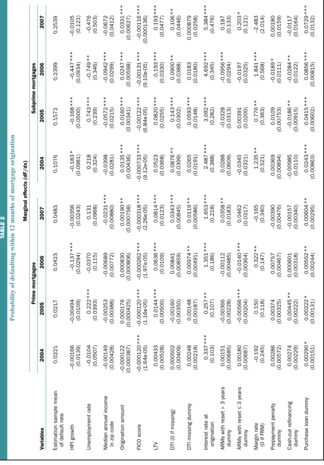
The results of the estimation are summarized in table 2. The first four columns of data depict estimates for prime loans originated in each of the four sample
years, and the next four columns contain the estimates for subprime loans. The juxtaposition of the data for the two market segments allows us to easily compare the importance of certain factors. The table presents estimates of the marginal effects of the explanatory variables, rather than the coefficients themselves. The marginal effects tell us how a one-unit change in each explanatory variable changes the probability that a loan defaults in its first 12 months, holding fixed the impact of the other explanatory variables. For dummy variables, the marginal effects show the change in the probability of default when the variable in question goes from zero to one.
The defaults of both prime and subprime loans are strongly associated with a number of key loan and borrower characteristics. These include the FICO score, the LTV, and the interest rate at origination. These vari-ables are strongly statistically significant in virtually every estimation year for each loan type. For instance, higher FICO scores are strongly associated with lower default probabilities. For prime loans, an increase of 100 points in the FICO score in 2004 is associated with about a 120-basis-point decrease in default likelihood (the estimated marginal effect of –0.00012, in the first column, sixth row of table 2, multiplied by 100). The same result is obtained for 2005. The point estimates of marginal effects for 2006 and 2007 increase about two-fold for prime loans, but so does the baseline sample default rate. For subprime loans, the estimated marginal effects are a full order of magnitude higher, implying that the same improvement in FICO scores generates a greater decline in subprime defaults, at least in ab-solute terms.
Similarly, higher LTV values have a strong posi-tive association with defaults for both loan types orig-inated in 2005, 2006, and 2007. For subprime loans, a rise in LTV generates a stronger absolute increase in loan defaults. It must be noted that the effect of the leverage on the likelihood of default may be understated by the LTV measure that we have. A better measure of how leveraged a borrower is on a given property would be the combined loan-to-value ratio (CLTV). The CLTV takes into account second-lien loans on the property in computing the ratio of indebtedness to the value of the underlying collateral. This variable is not available in the LPS data, however. If the practice of obtaining such “piggyback loans” is more prevalent in the sub-prime market, then the estimated coefficient for LTV for subprime loans may be biased downward.
At first glance, the interest rate at origination is similar to LTV and FICO score in having a strong sta-tistical and economic effect on both prime and sub-prime loan defaults in each origination year. What
stands out is the sheer magnitude of the estimated effects. However, one must be cautious in interpret-ing hypothetical marginal effects of the interest rate. While LTV and FICO score cover fairly wide ranges for both prime and subprime loans, interest rate values are more tightly distributed.22 For example, the stan-dard deviation of interest rates on prime loans across all years of our sample is 81 basis points: A one stan-dard deviation increase in the interest rate for prime loans would raise the average rate from 6.25 percent to 7.06 percent. The equivalent one standard deviation increase in interest rates for subprime loans would raise the average rate from 7.93 percent to 9.24 percent. If we see two loans with otherwise identical characteristics but one has a higher interest rate, a likely explanation is that the lender has additional information about the credit quality of the borrower and is charging a higher interest rate to take into account additional risk factors, over and above those that are captured by the borrower’s FICO score.
There are also a number of notable differences between the prime and subprime samples. Perhaps the most interesting finding is the different sensitivity of defaults to changes in home prices. For subprime loans, defaults are much lower when home price growth is higher for three out of the four sample years. This re-lationship is particularly striking for 2006 loan origi-nations, many of which experienced home price declines over their first 12 months. For prime loans, 2006 is the only year of origination in which changes in home prices are significantly correlated with loan defaults. These results suggest that, relative to subprime defaults, prime defaults have a weaker relationship with home prices, once key borrower and loan characteristics (LTV, FICO score, and so on) are taken into account.
The contrast between prime and subprime loans is even sharper for the debt-to-income ratio and loan margin rate. The DTI is widely considered to be one of the main determinants of loan affordability, since it relates household monthly income to debt service flows. The DTI for prime loans is not significantly correlated with defaults, except for loans originated in 2007, but it matters consistently for subprime loans. The absence of any measurable effects of DTI even on defaults of prime loans originated in 2006 can be interpreted as a sign of the resilience of prime borrowers who experi-enced significant changes in the prices of their homes.
The loan margin rate is one of the key terms in an ARM contract. It defines the spread to a reference rate (usually the London interbank offered rate, or Libor). At reset, the ARM’s interest rate goes up to the sum of Libor and the loan margin. The margin is set by the lender, and is often thought to capture additional aspects
of a borrower’s creditworthiness. This is consistent with the fact that the margin rate is, on average, sub-stantially higher for subprime borrowers (see table 1, p. 23). We find that this variable has no association with defaults among prime loans, with the exception of loans originated in 2006. In contrast, defaults on subprime loans originated in every year except 2007 are significantly higher for loans with higher margin rates, all else being equal. This suggests that, for the subprime borrower, the margin rate contains addition-al information on borrower quaddition-ality not reflected in FICO scores and other loan characteristics. It is also interesting that ARMs with introductory periods of three years or less—the most common mortgage con-tract in the subprime market—have the same correla-tion with subprime defaults as fixed-rate mortgages do. Put differently, once loan and borrower character-istics are accounted for, the choice of an ARM with a short introductory period is not associated with higher subprime defaults.
Several other results merit comment. For prime loans, being securitized within one month of origination (as opposed to remaining in the lender’s portfolio) is associated with lower defaults for loans made in 2004, 2005, and 2006. This does not necessarily mean that the securitization process has been successful in iden-tifying loans of higher quality. Since nearly all loans in the sample are securitized over the 12-month default horizon (see table 1, p. 23), the difference in defaults probably captures differences between fast-to-securi-tize and slow-to-securifast-to-securi-tize originators, rather than differences between securitized loans and those held on portfolio. We find similar results for securitized subprime loans made in 2005, 2006, and 2007. Sub-prime loans also have extremely high rates of eventual securitization, and the relationship between subprime default and securitization can be interpreted in the same way. This hints at the possibility that originators with business models focused on securitization are better at screening loan quality. These originators would have more to lose if their reputations were damaged by weak ex post performance of the loans they originated.
Finally, we note that purchase loans, as opposed to refinance loans, are consistently associated with higher defaults in nearly all sample years, in both the prime and subprime market segments. This may seem surprising, since borrowers who extract equity from their homes in cash-out refinancings may be particu-larly vulnerable to economic shocks and experience higher defaults as a result. However, not all cash-out refinancing is done by borrowers who need to finance current consumption. Since a prerequisite for any cash-out transaction is the availability of positive home
TABLE 2
Pr
obability of defaulting within 12 months of mortgage origination
Marginal effects (dF/dx) Prime mor tgages Subprime mor tgages Variables 2004 2005 2006 2007 2004 2005 2006 2007
Estimation sample mean
0.0221 0.0217 0.0423 0.0483 0.1076 0.1572 0.2399 0.2539
of default rate HPI growth
–0.00166 –0.00494 –0.137 *** –0.00356 –0.183 * –0.168 *** –0.447 *** –0.0105 (0.0139) (0.0109) (0.0294) (0.0243) (0.0981) (0.0500) (0.0934) (0.121) Unemplo yment rate –0.0104 0.222 *** –0.0370 0.131 0.218 0.743 *** –0.749 ** –0.476 (0.0507) (0.0393) (0.115) (0.0968) (0.324) (0.239) (0.346) (0.503)
Median annual income
–0.00149 –0.00253 –0.00689 –0.0231 *** –0.0398 –0.0572 *** –0.0942 *** –0.0672 in zip code (0.00428) (0.00388) (0.00772) (0.00880) (0.0281) (0.0215) (0.0299) (0.0412) Origination amount –0.000122 0.000176 0.000830 0.00190 ** 0.0135 *** 0.0160 *** 0.0247 *** 0.0331 *** (0.000387) (0.000425) (0.000806) (0.000758) (0.00436) (0.00341) (0.00598) (0.00627) FICO score –0.000120 *** –0.000120 *** –0.000262 *** –0.000318 *** –0.000733 *** –0.00122 *** –0.00131 *** –0.00116 *** (1.64e-05) (1.16e-05) (1.97e-05) (2.26e-05) (9.12e-05) (6.84e-05) (9.10e-05) (0.000136) LTV 0.00433 0.0144 *** 0.0636 *** 0.0814 *** 0.0523 0.0820 *** 0.193 *** 0.193 *** (0.00528) (0.00500) (0.0109) (0.0123) (0.0368) (0.0255) (0.0330) (0.0477) DTI (0 if missing) 0.000502 –0.00160 0.00841 0.0343 *** 0.0876 ** 0.143 *** 0.0900 ** 0.106 ** (0.00409) (0.00350) (0.00859) (0.00845) (0.0399) (0.0302) (0.0388) (0.0446)
DTI missing dumm
y 0.00248 0.00148 0.00974 ** 0.0119 ** 0.0265 0.0593 *** 0.0183 0.000879 (0.00218) (0.00187) (0.00491) (0.00586) (0.0191) (0.0148) (0.0180) (0.0258) Interest rate at 0.337 *** 0.257 ** 1.351 *** 1.653 *** 2.487 *** 3.092 *** 4.692 *** 5.384 *** origination (0.103) (0.107) (0.186) (0.218) (0.388) (0.282) (0.345) (0.476)
ARMs with reset > 3 year
s 0.00151 –0.00366 –0.00112 0.0358 ** 0.0288 –0.0328 –0.0956 *** 0.187 dumm y (0.00685) (0.00228) (0.00485) (0.0183) (0.0609) (0.0313) (0.0294) (0.133)
ARMs with reset
≤ 3 year s 0.00180 –0.00566 *** –0.0140 *** 0.0462 –0.0345 0.00391 –0.0197 0.203 * dumm y (0.00687) (0.00204) (0.00364) (0.0317) (0.0321) (0.0200) (0.0325) (0.121) Margin rate –0.192 0.150 0.322 ** –0.165 1.235 ** 0.776 ** 1.841 *** –2.483 (0 if FRM) (0.245) (0.118) (0.147) (0.340) (0.521) (0.363) (0.568) (2.014) Prepa yment penalty 0.00286 0.00374 0.00757 –0.00390 0.00369 0.0109 –0.0189 * 0.00180 dumm y (0.00572) (0.00325) (0.00467) (0.00476) (0.00894) (0.00753) (0.0111) (0.0159) Cash-out refinancing 0.00274 0.00445 ** 0.000601 –0.00157 –0.00985 –0.0186 ** –0.0284 ** –0.0117 dumm y (0.00229) (0.00222) (0.00318) (0.00340) (0.0110) (0.00915) (0.0122) (0.0164)
Purchase loan dumm
y 0.00290 * 0.00222 * 0.00552 ** 0.00604 ** 0.0243 *** 0.0415 *** 0.0856 *** 0.0729 *** (0.00151) (0.00131) (0.00244) (0.00295) (0.00863) (0.00602) (0.00815) (0.0132)
TABLE 2
(CONTINUED)
Pr
obability of defaulting within 12 months of mortgage origination
Marginal effects (dF/dx) Prime mor tgages Subprime mor tgages Variables 2004 2005 2006 2007 2004 2005 2006 2007 In vestment proper ty loan –0.000422 0.00468 0.000339 0.00159 –0.00612 –0.00102 –0.00164 0.0446 dumm y (0.00305) (0.00304) (0.00378) (0.00486) (0.0216 ) (0.0143) (0.0163) (0.0301) Confor
ming loan dumm
y –0.00290 –0.00667 *** –4.45e-05 0.00166 0.0154 0.0226 *** 0.0196 * 0.0119 (0.00190) (0.00184) (0.00288) (0.00344) (0.0120) (0.00864) (0.0107) (0.0184) GSE-securitized dumm y –0.0113 *** –0.00623 *** –0.0190 *** –0.00352 0.0255 –0.0312 –0.138 *** –0.00455 (0.00268) (0.00225) (0.00417) (0.00530) (0.0271) (0.0194) (0.0284) (0.0294) Private-label-securitized –0.00578 ** –0.000475 –0.00930 ** –0.000801 0.00680 –0.0860 *** –0.168 *** –0.0619 ** dumm y (0.00269) (0.00207) (0.00424) (0.00635) (0.0183) (0.0148) (0.0228) (0.0241) Obser vations 8,887 15,653 13,941 12,932 5,825 19,356 17,359 8,349 R-squared 0.2587 0.2364 0.1997 0.1962 0.1138 0.0934 0.0926 0.0745
*Significant at the 10 percent le
vel.
**Significant at the 5 percent le
vel.
***Significant at the 1 percent le
vel.
Notes: These are probit regressions with state fixed effects. Standard er
ror
s are in parentheses. The securitization status (GSE or private label) is measured during the fir
st month since origination. F
or definitions
of the variables,
see box 1 on p. 22.
Source: Author
s’ calculations based on data from Lender Processing Ser
vices (LPS) Applied Analytics.
equity, these borrowers, as a group, may have a greater incentive to avoid defaults to maintain this option for the future. In addition, purchase loans include first-time home buyers who, in retrospect, were buy-ing houses at the peak of the market and had little time to build up equity to offset subsequent price declines.
Comparisons across years and across loan types
Since table 2 contains regression estimates from multiple nonoverlapping samples, the comparison of the relative importance of the explanatory variables can be tricky. The distribution of loan characteristics varies from year to year and across prime and subprime loans. In addition, the baseline rates of actual de-faults are quite different across samples. Because of this, one cannot simply com-pare two point estimates and conclude that a bigger one indicates a stronger cor-respondence with defaults.
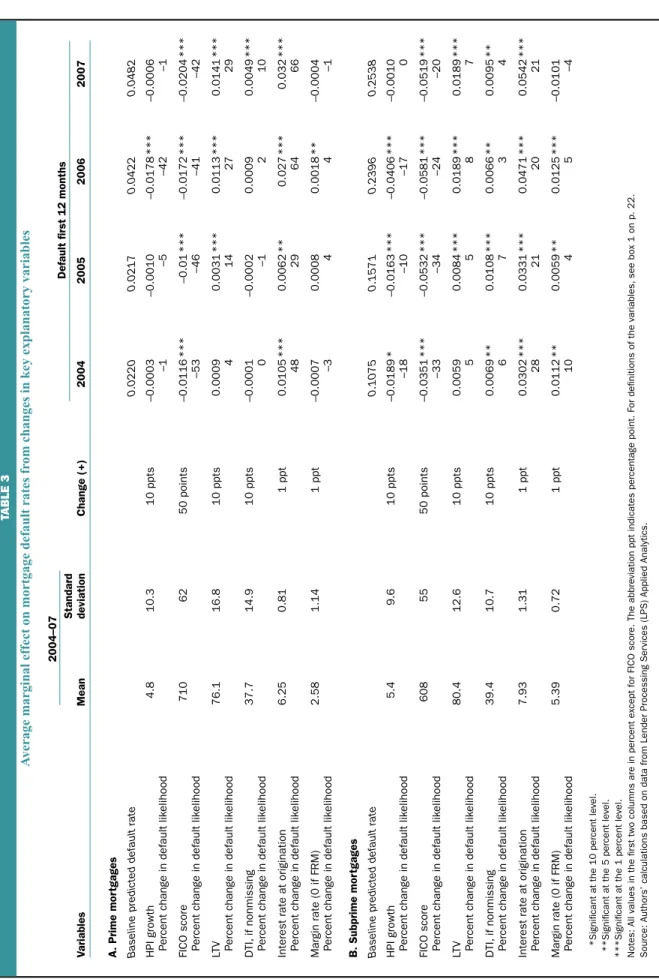
To compare the relative importance of the explanatory variables across the samples, we conduct the following exer-cise. For each independent variable, we change its value for each observation by a specified increment. Then, we compute the predicted sample default rate using estimated coefficients for each year of origination and loan type. We compare the new predicted default to the original one. The difference between the original pre-diction and the new one tells us the mar-ginal contribution of that variable to the overall default rate.23 We compare these figures across years and across prime loans (table 3, panel A) and subprime loans (table 3, panel B). For example, for 2004 prime loans we increase all FICO scores by 50 points, predict a new default rate, and compare it to the original default rate. The difference is –1.16 percentage points, or a 53 percent decrease in the likelihood of default for loans originated in 2004 (fourth column, second full row of table 3, panel A). For brevity, we look at just six key explanatory variables: HPI growth, FICO score, LTV, DTI, interest rate at
origination, and loan margin rate.24 Table 3
also reports the mean of the relevant vari-able, its standard deviation, and the absolute
change that we impose. We tried to keep the magni-tude of the absolute changes reasonably close to the standard deviations.
An increase of 10 percentage points in home price appreciation (HPI growth) substantially lowers default probabilities (first full row of each panel in table 3). This effect is more consistent for subprime loans origi-nated in various years, where it translates to decreases of between 10 percent and 18 percent relative to the baseline default rate in 2004, 2005, and 2006. For prime loans, the 10-percentage-point increase in the HPI has a big effect only for loans originated in 2006, where the estimates imply that defaults would have been 1.78 percentage points, or 42 percent, lower. The effect of FICO score stands out. A 50-point uniform increase in FICO scores (second full row of each panel) is asso-ciated with a 41 percent to 53 percent decline in pre-dicted default rates relative to the baseline for prime loans, and a 20 percent to 34 percent relative decline for subprime loans. The average marginal effects of the LTV are greater (in a relative sense) for prime loans than for subprime loans.25 Finally, higher interest rates at origination appear to generate incredible increases in defaults for both market segments. For instance, a 1 percentage point increase in interest rates translates into a jump in defaults on 2007 prime loans of more than 3 percentage points—a rise of 66 percent relative to the actual default rate. Increasing everyone’s interest rates by 1 percentage point is equivalent to a substan-tial deterioration in the quality of the borrower pool, and thus translates into much higher predicted defaults. As mentioned earlier, the DTI and the margin rate do not have strong associations with prime mortgage defaults. In contrast, higher values of these variables consis-tently indicate higher default rates for subprime mort-gages. However, the economic magnitude of marginal effects of DTI and the margin rate on defaults (fourth and sixth full rows of each panel) is somewhat muted. What if?
In this section, we use the estimates discussed previously to do two things. First, we examine how much (or how little) of the increase in mortgage de-faults from 2004 through 2007 can be explained by changes in the characteristics of loans and borrowers, as opposed to changes in the responsiveness of de-faults to those characteristics. Next, we examine how forecasts of prime and subprime mortgage defaults vary with different assumptions about the future path of home prices.
Predicted versus actual defaults
The descriptive regressions in the previous section provide insights into the factors that are associated with realized defaults for different types of loans originated in different years. An open question is how useful these relationships could have been in forecasting the defaults of future loans. To address this, we conduct the fol-lowing thought experiment. For each set of estimates, we compute predicted defaults using observed loan, borrower, and economic characteristics from other origination years. For instance, we take the relationship between borrower characteristics and loan character-istics that we estimate using data from prime loans originated in 2004 (the marginal effects reported in the first column of table 2, pp. 28–29) and see what it would imply for defaults for prime loans originated in 2007. In other words, we pick a particular year and
fix the relationship (that is, the estimated coefficients)
between defaults and characteristics, but let the charac-teristics vary as they actually did in the data. This ex-ercise lets us see to what extent higher defaults on loans originated in 2007 can be explained by changes in characteristics alone. We show these results in table 4, where this exercise is carried out separately for prime loans (panels A and B) and subprime loans (panels C and D). Panels A and C of the table show the predicted default rate for loans originated in each of the sample years (rows) using the coefficients estimated with data from each of the sample years (columns). The numbers in bold that run diagonally through the panels are pre-dictions that use characteristics and coefficients from the same year. A useful way to summarize the results is to look at predictions below and above the diagonal bold entries. Those below the diagonal bold entries are forecasts of future defaults using historical models (for example, relationships between characteristics and defaults from 2004 and characteristics from 2007). Those above the diagonal run this exercise in reverse—they ap-ply recent model estimates to loans from earlier years (for example, relationships between characteristics and defaults from 2007 and characteristics from 2004). These two groups of predictions are strikingly differ-ent in terms of their predictions relative to the actual realized default rates.
Perhaps the easiest way to see this is in panels B and D of table 4, which express predicted defaults as a percentage of realized defaults. The diagonal forecasts in those two panels are close to 100 percent. This is a feature of the estimation procedure. However, forward-looking forecasts—those below the diagonal bold entries—are nearly always less than 100 percent for both prime and subprime loans.26 This means that predic-tions based on relapredic-tionships between characteristics
TABLE 3
Average marginal effect on mortgage default rates fr
om changes in key explanatory variables
Standard Variables Mean de viation Change (+) 2004 2005 2006 2007 A. Prime mor tgages
Baseline predicted default rate
0.0220 0.0217 0.0422 0.0482 HPI growth 4.8 10.3 10 ppts –0.0003 –0.0010 –0.0178 *** –0.0006 P
ercent change in default lik
elihood –1 –5 –42 –1 FICO score 710 62 50 points –0.0116 *** –0.01 *** –0.0172 *** –0.0204 *** P
ercent change in default lik
elihood –53 –46 –41 –42 LTV 76.1 16.8 10 ppts 0.0009 0.0031 *** 0.0113 *** 0.0141 *** P
ercent change in default lik
elihood 4 14 27 29 DTI, if nonmissing 37.7 14.9 10 ppts –0.0001 –0.0002 0.0009 0.0049 *** P
ercent change in default lik
elihood 0 –1 2 10
Interest rate at origination
6.25 0.81 1 ppt 0.0105 *** 0.0062 ** 0.027 *** 0.032 *** P
ercent change in default lik
elihood 48 29 64 66 Margin rate (0 if FRM) 2.58 1.14 1 ppt –0.0007 0.0008 0.0018 ** –0.0004 P
ercent change in default lik
elihood –3 4 4 –1 B. Subprime mor tgages
Baseline predicted default rate
0.1075 0.1571 0.2396 0.2538 HPI growth 5.4 9.6 10 ppts –0.0189 * –0.0163 *** –0.0406 *** –0.0010 P
ercent change in default lik
elihood –18 –10 –17 0 FICO score 608 55 50 points –0.0351 *** –0.0532 *** –0.0581 *** –0.0519 *** P
ercent change in default lik
elihood –33 –34 –24 –20 LTV 80.4 12.6 10 ppts 0.0059 0.0084 *** 0.0189 *** 0.0189 *** P
ercent change in default lik
elihood 5 5 8 7 DTI, if nonmissing 39.4 10.7 10 ppts 0.0069 ** 0.0108 *** 0.0066 ** 0.0095 ** P
ercent change in default lik
elihood 6 7 3 4
Interest rate at origination
7.93 1.31 1 ppt 0.0302 *** 0.0331 *** 0.0471 *** 0.0542 *** P
ercent change in default lik
elihood 28 21 20 21 Margin rate (0 if FRM) 5.39 0.72 1 ppt 0.0112 ** 0.0059 ** 0.0125 *** –0.0101 P
ercent change in default lik
elihood 10 4 5 –4
*Significant at the 10 percent le
vel.
**Significant at the 5 percent le
vel.
***Significant at the 1 percent le
vel.
Notes: All values in the fir
st two columns are in percent except for FICO score. The abbre
viation ppt indicates percentage point. F
or definitions of the variables,
see box 1 on p. 22.
Source: Author
s’ calculations based on data from Lender Processing Ser
vices (LPS) Applied Analytics.
Default fir
st 12 months
TABLE 4
Predicted probability of defaulting within 12 months of mortgage origination
Prediction model coefficients from
Mortgages originated in Actual default rate 2004 2005 2006 2007
( - - - percent - - - )
A. Prime mortgages: Predicted default rate
2004 2.21 2.20 2.55 1.47 2.86
2005 2.17 2.04 2.17 1.72 3.77
2006 4.23 3.09 3.08 4.22 5.62
2007 4.83 3.54 3.49 5.82 4.82
B. Prime mortgages: Predicted default rate as percentage of actual default rate
2004 100 99.89 115.63 66.63 129.72
2005 100 93.94 99.77 79.15 173.55
2006 100 72.98 72.68 99.73 132.71
2007 100 73.32 72.11 120.45 99.77
C. Subprime mortgages: Predicted default rate
2004 10.76 10.75 13.72 13.26 16.62
2005 15.72 13.56 15.71 16.78 19.93
2006 23.99 19.92 20.68 23.96 24.95
2007 25.39 22.27 23.06 25.49 25.38
D. Subprime mortgages: Predicted default rate as percentage of actual default rate
2004 100 99.83 127.48 123.21 154.41
2005 100 86.31 99.98 106.80 126.78
2006 100 83.04 86.20 99.89 104.01
2007 100 87.70 90.80 100.40 99.97
Notes: Average predicted default rate for mortgages, using estimated coefficients from different mortgage origination years. Bold numbers are predictions that use characteristics and coefficients from the same year. See the text for further details.
Source: Authors’ calculations based on data from Lender Processing Services (LPS) Applied Analytics.
and defaults from 2004 and 2005 uniformly underpredict defaults in 2006 and 2007. The underprediction is more dramatic for prime loans, where less than 75 percent of the realized defaults in 2006 and 2007 are accounted for by the “old” relationships between characteristics and defaults. Even for subprime loans, the shortfall is substantial, suggesting increased defaults cannot be accounted for by changes in loan characteristics alone. The relationship between observable loan and economic characteristics and defaults appears to have changed for loans originated after 2005. The sharp rise in the default rate cannot be explained just by looser under-writing standards or by changes in the composition of loan contracts.
In contrast, the backward-looking forecasts— those above the diagonal bold entries—are typically greater than 100 percent. This means that the world described by defaults observed in 2006 and 2007 would have resulted in defaults higher than observed in 2004 and 2005. This overprediction holds uniform-ly for subprime mortgages, but not for the predictions based on the 2006 model of prime defaults. More-over, the overprediction is particularly severe for the
2007-based model coefficients, again suggesting a structural difference in the determinants of loan de-faults that occurred after the rapid reversal in home price appreciation.
What role do home prices play?
We turn our attention now to the role of home prices. We know that home prices were increasing very rapidly in 2004 and 2005 and began to fall quite dramatically beginning in 2006. A closer look at the potential impact of this shock may help to illuminate why defaults of both prime and subprime mortgages increased so much. We are also interested in refining the discussion by being very clear about what infor-mation would have been available to analysts at dif-ferent points in time. This will allow us to gauge the extent to which market participants were “surprised” by the performance of prime and subprime loans originated in 2006 and 2007.
The results in table 4 give the impression that an analyst would be able to predict 2006 loan defaults, using 2005 model estimates. In reality, this would not have been possible because the model of 2005 defaults
TABLE 5
Mortgage default rate forecasts under different assumptions for the future path of home prices
Predictions
for mortgages Actual
Model year coefficients originated in default rate Scenario I Scenario II Scenario III
( - - - percent - - - )
A. Default rate forecasts for prime mortgages
2004 2006 4.23 3.09 3.03 3.07
2005 2007 4.83 3.49 3.39 3.43
B. Default rate forecasts for subprime mortgages
2004 2006 23.99 19.92 17.47 20.32
2005 2007 25.39 23.06 21.51 22.18
Prime mortgages Subprime mortgages All mortgages Mortgages originated in Scenario I Scenario II Scenario I Scenario II Scenario III
( - - - percent - - - )
C. Average HPI growth rates assumed in each scenario
2004 13.44 10.63 13.99 12.89 0.00
2005 9.10 14.30 9.70 15.00 0.00
2006 1.94 9.57 1.52 9.87 0.00
2007 –4.19 2.65 –3.94 3.29 0.00
Notes: The forecast horizon is 12 months since mortgage origination. HPI means House Price Index from the Federal Housing Finance Agency. Scenario I is perfect foresight; it uses actual realized HPI growth. Scenario II is a simple extrapolation; it uses the HPI growth rate from the preceding 12 months. Scenario III assumes zero HPI growth for the forecasting period. See the text for further details.
Source: Authors’ calculations based on data from Lender Processing Services (LPS) Applied Analytics.
could only be estimated in full in December 2006 when loans made in December 2005 had been ob-served for a full 12 months. Moreover, some of the key variables—notably, future growth in the HPI—are not of course available at the time a loan is made. To create estimates of default predictions that take into account only the available information, we conduct a series of experiments that are reported in table 5.
In panels A and B of table 5, the first row presents predicted defaults for 2006, using coefficients from estimates of default for loans made in 2004. The in-formation necessary to do this exercise would not have been available at the beginning of 2006. In panels A and B of table 5, the second row does the same for 2007 defaults, using coefficients from estimates of default for loans made in 2005. Each of the scenarios uses the same coefficients (2004 or 2005), but differs in assump-tions about HPI growth. Scenario I assumes that the analyst can perfectly predict future home prices (this simply restates the appropriate value from table 4). Scenario II assumes that an analyst forecasts that the MSA-specific HPI growth in a given year will change by exactly as much as it did in the most recent observ-able 12-month period. In other words, for a particular MSA, HPI growth in 2006 will look just like it did in
2005, and this growth in 2007 will look just like it did in 2006. In scenario III, the hypothetical analyst becomes very pessimistic and assumes that house prices in 2006 and 2007 will not grow at all. Panel C of table 5 sum-marizes the average MSA-level HPI growth rates as-sumed in each scenario for prime and subprime loans.
The results for prime loans (table 5, panel A) suggest that varying assumptions about HPI growth has little effect on predicted default rates. Whether one uses past experience to extrapolate future home price growth or arbitrarily sets the growth rate to zero, the model substantially underpredicts the actual default rate. The historical experience in the prime market for loans originated in 2004 and 2005 suggested that there was essentially no relationship between home price appre-ciation and loan defaults. Using the experience of mort-gages originated during this period together with any assumption about HPI growth would not have helped analysts forecast the spike in prime loan defaults. What would have been helpful would have been if an analyst could have foreseen that prime mortgages might respond to home prices the way subprime mortgages did.
Even when home price appreciation was relatively high during 2004 and 2005, default rates among sub-prime borrowers were quite sensitive to home prices.
Indeed, the results for the subprime loans, shown in table 5, panel B, suggest that assuming zero price growth would have gone a long way in closing the gap be-tween forecasts based on simple extrapolation of past growth and actual defaults. This is especially true for loans originated during 2006, which proved to be the pivotal year for home prices and loan performance. For those loans, extrapolation of past trends using coeffi-cients from estimates of default for loans made in 2004 predicted default rates of 17.5 percent. With the assump-tion of zero growth, the same model produced default rates of 20.3 percent, much closer to the actual rate of 24 percent. Even relying on the somewhat stale coef-ficient estimates, it appears to have been possible to forecast a sharp deterioration in default rates on sub-prime loans with fairly mild HPI growth assumptions. However, the same cannot be said for prime loans. Conclusion
We have analyzed the default experience of prime and subprime loans originated over the period 2004–07. Similar to other studies, we document some decline in underwriting standards during this period for both prime and subprime loans. We also find that character-istics such as the loan-to-value ratio, FICO score, and interest rate at origination are important predictors of defaults for both prime and subprime loans. However,
changes in loan and borrower characteristics are not enough to have predicted the incredible increase we have seen in prime and subprime mortgage defaults. While changes in borrower and loan characteristics can get us closer to observed default rates for sub-prime loans than they can for sub-prime loans, for both market segments there were other factors at work.
Home prices play a very important role in deter-mining mortgage outcomes; this became particularly evident for subprime loans by the end of 2005. For prime loans, it is only when we analyze data through the end of 2007 (that is, evaluate the performance of loans originated in 2006) that we are able to docu-ment this sensitivity. Even very pessimistic assump-tions about the future path of home prices would not have been enough to substantially improve contem-poraneous forecasts of prime mortgage defaults for loans made in 2006 and 2007. In hindsight, of course, it appears self-evident that the relationships between HPI growth and defaults on prime loans might be dif-ferent in periods with declining home prices. However, recognizing this in real time would not have been possible using the available data from the recent past. It could, perhaps, have been done by analyzing data that included earlier episodes of substantial regional home price declines.