Three Essays on Monetary Policy

UC San Diego

UC San Diego Electronic Theses and Dissertations

Title

Three Essays on Monetary Policy

Permalink https://escholarship.org/uc/item/221242ww Author Zhang, Xu Publication Date 2019 Peer reviewed|Thesis/dissertation

UNIVERSITY OF CALIFORNIA SAN DIEGO

Three Essays on Monetary Policy

A dissertation submitted in partial satisfaction of the requirements for the degree

Doctor of Philosophy in Economics by Xu Zhang Committee in charge:

Professor James Hamilton, Chair Professor David Lagakos

Professor Jun Liu

Professor Michael Malvin Professor Tommaso Porzio Professor Rossen Valkanov Professor Johannes Wieland

Copyright Xu Zhang, 2019 All rights reserved.

The Dissertation of Xu Zhang is approved, and it is acceptable in quality and form for publication on microfilm and electronically:

Chair

University of California San Diego 2019

DEDICATION

I dedicate my dissertation work to my family and many friends, whose support and

TABLE OF CONTENTS

Signature Page . . . iii

Dedication . . . iv

Table of Contents . . . v

List of Figures . . . vii

List of Tables . . . ix

Acknowledgements . . . x

Vita . . . xi

Abstract of the Dissertation . . . xii

Chapter 1 Disentangling the Information Effects in the Federal Reserve’s Monetary Policy Announcements . . . 1

1.1 Introduction . . . 1

1.2 Existing approaches and the problem . . . 4

1.3 Construction of the new measure . . . 11

1.4 Effects of the monetary policy surprise . . . 13

1.4.1 Response of private sector forecast . . . 13

1.4.2 Comovement of stock price and monetary policy surprise . . . 13

1.4.3 Application in a proxy SVAR framework . . . 14

1.5 Conclusion . . . 15

Chapter 2 Evaluating the Effects of Forward Guidance and Large-scale Asset Purchases 21 2.1 Introduction . . . 21

2.2 A Structural Model . . . 27

2.2.1 Households . . . 28

2.2.2 Banks . . . 31

2.2.3 Central bank’s asset purchases . . . 33

2.2.4 Aggregation . . . 33

2.2.5 The Production Sector . . . 34

2.2.6 Monetary Policy . . . 37

2.2.7 Government, Resource Constraint and Equilibrium . . . 39

2.3 Calibration and Simulation of the Structural Model . . . 39

2.3.1 Calibration . . . 39

2.3.2 Solution Method . . . 42

2.3.3 Crisis Experiment . . . 42

2.4 Yield Curve Interpolation . . . 44

2.4.2 Yield curve interpolation at the lower bound . . . 46

2.4.3 Calibration for the yield curve interpolation . . . 46

2.5 Decomposition of the Federal Reserve’s announcement . . . 48

2.5.1 Information and monetary policy components of the announcement . . . . 48

2.5.2 Decomposition of monetary policy component into forward guidance and LSAP . . . 49

2.5.3 Data . . . 50

2.5.4 Estimated size of forward guidance and LSAP . . . 51

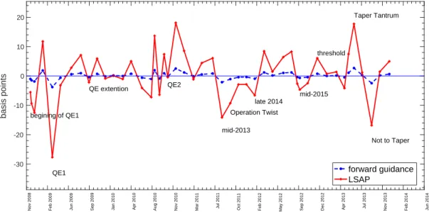
2.5.5 Estimated contribution of forward guidance and LSAP to the interest rates 51 2.5.6 Estimated contribution of forward guidance and LSAP to the real activities 51 2.6 Unconventional Monetary Policy on Several Key FOMC Announcement Days . 52 2.6.1 QE I phase (November 2008 to March 2010) . . . 52

2.6.2 QE II phase (November 2010 to June 2011) . . . 54

2.6.3 Mid-2013 phase (November 2010 to June 2011) . . . 54

2.6.4 “Operation Twist” (September 2011 to August 2012) . . . 55

2.6.5 QE III phase (September 2012 to May 2013) . . . 55

2.6.6 Tapering (June 2013 to October 2014) . . . 56

2.7 Discussion . . . 57

2.7.1 The importance of isolating the monetary policy component . . . 57

2.7.2 Robustness check . . . 57

2.8 Conclusion . . . 58

Chapter 3 Monetary Policy and Household Balance Sheet Heterogeneity . . . 86

3.1 Introduction . . . 86

3.2 Data . . . 89

3.2.1 Household balance sheet . . . 90

3.2.2 Household labor market outcome . . . 91

3.2.3 Household expenditure . . . 92

3.2.4 Monetary policy surprises . . . 92

3.3 Empirical methodology . . . 92

3.3.1 Baseline specification . . . 92

3.3.2 Specification I: age . . . 94

3.3.3 Specification II: homeownership . . . 94

3.3.4 Specification III: “wealthy” hand-to-mouth . . . 95

3.3.5 Specification IV: home equity . . . 96

3.3.6 Specification V: Loan to Value ratio . . . 97

3.3.7 Specification VI: home equity and Loan to Value ratio . . . 97

3.4 Conclusion . . . 97

LIST OF FIGURES

Figure 1.1. 12-month Backward Rolling Window of Cumulative Monetary Shocks . . . 16

Figure 1.2. Impulse Responses Using the New Measure, PC1 and Romer-Romer . . . . 17

Figure 2.1. Estimated Size of Each Shock Type . . . 60

Figure 2.2. Crisis Experiment . . . 61

Figure 2.3. Effects of Forward Guidance and LSAP Shocks . . . 62

Figure 2.4. Difference Between Fitted Yield Curves . . . 63

Figure 2.5. Estimated Effects on 10-year Treasury Yield . . . 64

Figure 2.6. Estimated Effects on 10-year Treasury Yield . . . 65

Figure 2.7. Estimated Effects on 11/25/2008 . . . 66

Figure 2.8. Estimated Effects on 12/16/2008 . . . 67

Figure 2.9. Estimated Effects on 01/28/2009 . . . 68

Figure 2.10. Estimated Effects on 08/09/2011 . . . 69

Figure 2.11. Estimated Effects on 09/21/2011 . . . 70

Figure 2.12. Estimated Effects on 06/19/2013 . . . 71

Figure 2.13. Estimated Effects on 12/18/2013 . . . 72

Figure 2.14. Difference Between Fitted Yield Curves When Initial Condition Varies . . . 73

Figure 2.15. Difference Between Fitted Yield Curves When the Definition of One Unit Shock Varies . . . 74

Figure 2.16. Estimated Effects on 10-year Treasury Yield When the Definition of One Unit Shock Varies . . . 75

Figure 2.17. Difference Between Fitted Yield Curves When Forward Guidance Persis-tence Varies . . . 76

Figure 2.18. Difference Between Fitted Yield Curves When Forward Guidance Horizon Varies . . . 77

Figure 3.2. Ratio of Mortgage Holder in the Population . . . 100

Figure 3.3. Ratio of Renter in the Population . . . 101

Figure 3.4. Unemployment Ratio in the Population . . . 102

Figure 3.5. Labor Force Participation Ratio in the Population . . . 103

Figure 3.6. Cumulative Monetary Policy Shock . . . 104

Figure 3.7. 25th Quantile Asset Composition Over Time by Housing Status . . . 105

Figure 3.8. Median Quantile Asset Composition Over Time by Housing Status . . . 106

Figure 3.9. 75th Quantile Asset Composition Over Time by Housing Status . . . 107

LIST OF TABLES

Table 1.1. Regression on NBER Recession Indicator . . . 18

Table 1.2. Regressions Estimating Private Forecast Responses to Various Measures of Contractionary Monetary Policy Shocks . . . 19

Table 1.3. % of Days Where S&P 500 Moves in the Opposite Direction with Monetary Policy Shocks . . . 20

Table 2.1. Parameter Values . . . 78

Table 2.2. Data and Model mplied yield curve, in annualized percentage points . . . 81

Table 2.3. Unconventional Monetary Policy on Several Key FOMC Announcement Days . . . 82

Table 3.1. Household Balance Sheet . . . 109

Table 3.2. Summary Statistics for SIPP Cross-sectional Homeowner with Debt . . . 110

Table 3.3. Summary Statistics for SIPP Cross-sectional Homeowner without Debt . . . 111

Table 3.4. Summary Statistics for SIPP Cross-sectional Private Renter . . . 112

Table 3.5. Baseline Specification . . . 113

Table 3.6. Specification I, Age . . . 114

Table 3.7. Specification II, Homeownership . . . 115

Table 3.8. Specification III(i), Hand to Mouth Household . . . 116

Table 3.9. Specification III(ii), “Wealthy” Hand to Mouth Household . . . 117

Table 3.10. Specification IV, Home Equity . . . 118

Table 3.11. Specification V, Loan to Value Ratio . . . 119

ACKNOWLEDGEMENTS

I would like to acknowledge Professor James Hamilton for his support as the chair of my committee. Through multiple drafts, his guidance has proved to be invaluable.

Many additional thanks to Johannes Wieland, David Lagakos, Tommaso Porzio and participants in the UCSD macroeconomics seminar. Your time, thoughts, and feedback helped me immensely throughout this process.

VITA

2011 Bachelor of Arts, Central University of Finance and Economics

2013 Master of Arts, Peking University

ABSTRACT OF THE DISSERTATION

Three Essays on Monetary Policy

by

Xu Zhang

Doctor of Philosophy in Economics

University of California San Diego, 2019

Professor James Hamilton, Chair

This dissertation studies the identification of monetary policy and the effects of monetary policy on the macroeconomy.

Chapter 1 provides a new methodology to identify monetary policy shock. Federal Reserve announcements contain information about both economic fundamentals and monetary policy. My paper proposes to disentangle the information effects using Federal Reserve’s forecasts about the macroeconomy and constructs a new measure of monetary policy shocks. The new shock series is consistent with the traditional view.

Chapter 2 investigates the effects of unconventional monetary policy when the nominal interest rate reaches the zero lower bound. There are two types of monetary policy, i.e. forward

guidance and large-scale asset purchases. I identify the separate contributions of each monetary policy shock to the effects on yield curve and macroeconomy.

Chapter 3 studies the effects of monetary policy on the household behavior. I look at how households with heterogeneous balance sheet composition would make their decisions in response to monetary policy interventions, and to what extent and this could affect the aggregate economy. I provide empirical analysis using household-level data, and document empirical stylized facts that can be used to evaluate different theoretical transmission channels of monetary policy.

Chapter 1

Disentangling the Information Effects in

the Federal Reserve’s Monetary Policy

Announcements

Abstract

Federal Reserve announcements affect private sector beliefs in two different ways, reveal-ing information about both economic fundamentals and monetary policy. This paper separates the information revelation from the effect of policy by combining the high-frequency multidimen-sional approach of G¨urkaynak et al. (2005) with Greenbook measures of the Fed’s information as in Romer and Romer (2004). The new shock series is consistent with the traditional view. In contrast to existing measures, a contractionary shock causes an upward revision in private forecasts of unemployment, a downward revision in private forecasts of inflation, and a decline in stock price.

1.1

Introduction

A number of approaches have been suggested for measuring a monetary policy shock. Kuttner (2001) use the daily change in the current month federal funds futures contract on the day of a Federal Open Market Committee (FOMC) meeting. Gertler and Karadi (2015) use the change in the 3-month-ahead federal funds futures contract. G¨urkaynak et al. (2005) calculated principal components of the current and 3-month-ahead federal funds future along with 6-month,

9-month, and 1-year ahead Eurodollar futures. Romer and Romer (2004) use the change in the Fed’s intended target that could not be predicted on the basis of the Fed’s Greenbook forecasts of inflation, GDP, and unemployment. Miranda-Agrippino and Ricco (2018) use the component of the change in the 3-month-ahead fed funds futures in a 30-minute window around FOMC announcements that could not be predicted using Greenbook forecasts.

In this paper I present evidence that none of these measures completely corrects for the Fed information effect. The first four measures are all statistically significantly negative on average during NBER recessions. The Fed was surprising the market by lowering rates at these times in response to weak economic fundamentals that the Fed recognized but the market did not. This means that existing measures are conflating the effects of monetary policy, the effects of information revelation, and the effects of the recession itself. I extend the analysis of Campbell et al. (2012) and Nakamura and Steinsson (2018) to find that revisions to the Blue Chip consensus forecasts of unemployment typically fall after a contractionary monetary policy shock according to all of the measures except for Romer and Romer, the opposite response from that predicted for a true contractionary monetary shock, and a response suggesting that revelation of the Fed’s information about economic fundamentals is likely an important component of what is treated as a shock to monetary policy. I extend the analysis of Cieslak and Schrimpf (2018) and Jaroci´nski and Karadi (2018), finding that about half the time, stock prices rise at the time of a contractionary monetary policy shock according to the Kutter, Gertler-Karadi, or Romer-Romer measures. Finally, the federal funds rate, current month feral funds futures rate and the 3-month-ahead fed funds futures rate exhibited essentially no variation over 2009 to 2014, meaning that the Kuttner, Gertler-Karadi, Romer-Romer, and Miranda-Agrippino-Ricco measures do not exist for this important subsample. It will create bias when calculating the principal components in the extended sample.

I develop a new measure that solves all of these problems, combining the multidimen-sional aspect of monetary policy information noted by G¨urkaynak et al. (2005) with the use of Greenbook forecasts by Romer and Romer (2004) and Miranda-Agrippino and Ricco (2018)

and exploiting the basic insight of using high-frequency observations for identification that is common to all of the above measures. I use separate regressions to isolate the component of the change on the day of an FOMC announcement of each of the five different fed funds and Eurodollar futures that could not have been predicted on the basis of Greenbook forecasts. I next calculate the principal component of this vector using an unbalanced panel approach that takes into account the lack of variability of the shorter horizon contracts during 2009-2014. In contrast to the other five measures, this measure is actually slightly positive on average (though far from statistically significant) during NBER recessions. It is the only measure for which revisions to the Blue Chip forecasts of both inflation and unemployment tend to change in the direction predicted for a monetary expansion or contraction. And about 2/3 of the time, stock and bond prices move together in the way predicted by theory. I use the new measure to revisit the structural vector autoregression of Gertler and Karadi (2015) and find that the new measure eliminates both the “price puzzle” and the “output puzzle” (responses to a monetary shock of the opposite sign predicted by theory) that is sometimes found using other measures. Given the 5-year delay in releasing Greenbook forecasts, the most recent value for the new measure is 2013:m12, though this still extends the usable sample by at least 4 years beyond that available for the Kuttner, Gertler-Karadi, Romer-Romer, or Miranda-Agrippino-Ricco measures.

This paper contributes to several important literatures. First, it adds to the monetary policy identification literature. This includes the VAR studies such as Christiano et al. (1999) and also the work of Romer and Romer (2004). More recent studies provide lots of evidence that monetary policy news is multi-dimensional. For example, G¨urkaynak et al. (2005) construct a “current federal funds rate target” factor and a “future path of policy” factor. Campbell et al. (2012) distinguish between Delphic and Odyssean monetary policy, where the Delphic type publicly states central banks’ macroeconomic performance forecast whereas the Odyssean type publicly commits the policymaker’s future action. To separate the non-information movement, Campbell et al. (2012) estimate a monetary policy rule with anticipated shocks. Nakamura and Steinsson (2018) model Fed’s information as beliefs about the path of the “natural rate of interest”

and estimate the structural model using real rates. To disentangle the two components, I provide a method that combines the high-frequency approach of G¨urkaynak et al. (2005) and Romer and Romer (2004)’s narrative approach. It is easy to implement and survives the prevailing tests in the literature.

My paper also contributes to the literature regarding the assessment of the effects of the unconventional monetary policies. Many of the world’s largest economies have experienced the zero short-term nominal interest rate over the last decade. It’s hard to find a measure for monetary policy surprises during this period. In addition, as Hamilton (2018) documents, like conventional monetary policy announcement, the Fed’s unconventional monetary policy announcements also contain Fed’s assessment of economic fundamentals. Since I use longer term federal funds futures to construct the measure, it survives the zero lower bound period.

The remainder of the paper proceeds as follows. I review the literature on the monetary policy identification in Section 1.2. In section 1.3, I describe the procedure to construct the monetary policy shock. Section 1.4 describes the effects of monetary policy using the new measure and applies the new measure to previous studies. Section 3.4 concludes.

1.2

Existing approaches and the problem

A number of studies have proposed alternative methods to measure a monetary policy shock. In this section I will review the five existing approaches and evaluate their performance.

Surprise in the federal funds rate target (MP1). The high-frequency identification approach was pioneered by Kuttner (2001). Under the identifying assumption that no other shocks affect the expectation for federal funds rate around the 30-minute window of FOMC announcement, the surprise in the target rate is measured as the daily change in the spot-month federal funds future rate (FF1), scaled up to reflect the number of days affected by the change. This monetary policy shock is called MP1 in the literature.

(and will do the same for all the other measures presented below) such that its effect on the daily

two-year nominal Treasury yield is equal to 100 basis points.1

To convert the shock series into monthly frequency, I assign each shock to the month in which the corresponding FOMC announcements are made. If there are two meetings in a month, I sum the shocks. If there are no meetings in a month, I record the shock as zero for that month. Monetary surprises are supposed to capture only unanticipated movements in interest rates. However, the mean of the MP1 series is nonzero, and it is serially correlated. After 2008, the MP1 didn’t vary much and was almost zero between 2009 and 2014. For this reason, I restrict the sample period of MP1 to be between 1990:1m and 2008:12m.

In the upper left panel of Figure 1.1, I plot the cumulative change in MP1 over a 12-month period using just the days of FOMC announcements. The shaded areas represent NBER-defined recessions for the U.S. economy. The Fed was surprising the market with lower interest rates during the recessions, and it was doing this because it saw the economy as weaker than many private analysts recognized at the time. To quantify this observation, I regress the monetary policy surprises on the NBER recession indicator and look at the regression coefficient. The regression equation is

MPSt =βRecessiont+εt (1.1)

where MPSt is the monetary policy surprise in montht. In the case of Kuttner (2001),

it is represented by the MP1t. Recessiont is a binary variable equal to 1 if the the montht is a

NBER recession month and equal to zero otherwise.

As shown in Table 1.1, the estimatedβ is -2.66 and is statistically significant at the

1% level. If one uses the MP1 to study the correlation between monetary shock and economic variables of interest, it will in part reflect the effect of the recession, not the effect of actions by

1_{The daily zero-coupon nominal Treasury yields are obtained from G¨urkaynak et al. (2007) dataset. Swanson}

and Williams (2014) provide evidence that the zero lower bound was not a constraint on the Federal Reserve’s ability to manipulate the two-year Treasury yield.

the Fed.

Next I look at whether the measure of MP1 includes an information effect. I follow Campbell et al. (2012) and estimate the responses of revisions of inflation and unemployment rate forecasts to the proposed monetary policy measure. The regression equation is

4yh_t+1=βhMPSt+εt+1 (1.2)

where4yh_t+1is the revision of the h-quarter-ahead Blue Chip consensus forecast of inflation and unemployment rate at the beginning of montht+1, andh=0,1,2,3,4.

Table 1.2 presents the regression result.2 In theory, a true contractionary monetary policy

shock should increase unemployment rate expectation and decrease the inflation expectation. However, most coefficients in column 1 show the opposite direction. The interpretation is that part of what happens is the Fed raises the interest rate because it sees fundamentals as stronger, and the private forecasts respond to the signal by being more optimistic about the the fundamentals.

Cieslak and Schrimpf (2018) and Jaroci´nski and Karadi (2018) look at the problem from the perspective of the comovement of S&P 500 with bond yields. Again, a true contractionary monetary policy shock should raise interest rates and depress output, both of which should lower stock prices. A contractionary monetary policy shock again seems to be interpreted by private forecasters as expansionary. However, as Table 3 shows, on 51% of all the announcement days do MP1 and the intraday change in S&P 500 co-move in the “correct” direction. This number decreases to 45% if we use the daily change in S&P 500.

Change in 3-month ahead Federal funds futures (4FF4). Gertler and Karadi (2015)

use the three month ahead funds rate future surprise (4FF4) around the 30-minute of Fed’s

2_{Blue Chip Economic Indicator survey is conducted between the 2nd and the 7th day of each month. The}

monetary surprise data I use for this regression is restricted to include only the announcements made after the first week of the calendar month. The result is robust if I use the observations where the entire month’s announcements are made after the first week of the calendar month.

announcement to identify monetary policy shock.

I plot the 12-month backward-rolling window cumulative change in the first row second

column of Figure 1.1. 4FF4 didn’t vary considerably and was almost zero between 2009 and

2013, which will make it impossible to use as an instrument during the Great Recession period. The sample period is 1990:1m-2008:12m.

From the figure as well as Table 1.1, we see that4FF4 is more likely to be negative

during the NEBR recession months. Column 2 of Table 1.2 presents the regression result of

equation 1.2 with the monetary policy surprise MPS measured by4FF4. Still, the contractionary

monetary policy looks like expansionary one. Table 1.3 shows that MP1 and the intraday change in S&P 500 move together as predicted on only 52% of announcement days. This number falls to 48% if we use the daily change in S&P 500.

Instrument set of futures (MP1, MP2, 4ED2, 4ED3, 4ED4). G¨urkaynak et al.

(2005) find that the FOMC statements affect the financial market through current policy action along with influence on the market expectations of future policy actions. They suggest to use mixed horizons of futures data to measure the response of market expectations. I follow the literature and use the following instrument set: the surprises in the current month’s fed funds futures with a scale factor to account for the timing of FOMC meetings within the month (MP1), in the three-month ahead monthly fed funds futures (also scaled, known as MP2), and in the six-month, nine-month and year ahead futures on three month Eurodollar deposits (ED2, ED3, ED4) on the days of FOMC announcement.

The sample period in G¨urkaynak et al. (2005) is from 1990:1m to 2004:12m, and Nakamura and Steinsson (2018) use the sample period 1995:1m - 2014:3m. I use the extended sample period 1990:1m -2018:12m, take the first principal component of the balanced panel, and rescale it such that the effect on the two-year nominal Treasury yield is equal to 100 basis points. This shock is called PC1.

One problem of applying G¨urkaynak et al. (2005)’s principal components idea to longer samples is that short term federal funds futures, and thus the MP1 and MP2 were unresponsive

during the Great Recession. Taking the principal component of the balanced sample will generate bias, especially for the recession period. In middle panel of Figure 1.1, I compare the PC1 with a modified PC1 which is calculated using the expectation maximum (EM) algorithm developed in Stock and Watson (2002) where MP1 and MP2 are treated as missing during the recession.

Let’s take look at the performance of the PC1. Again, the coefficient in Table 1.1 indicates the PC1 is more likely to be negative during the recession. And if I use the modified PC1, the result still holds. The coefficients in Column 3 of Table 1.2 are usually the opposite of what they should be. Table 1.3 shows PC1 and the intraday change in S&P 500 move together as predicted on 71% of announcement days. The results won’t change much if using the modified PC1 because these analysis is conducted for the sample period 1990:m1 - 2007:m12.

The Romer-Romer (RR) shock. The seminal empirical paper on Fed information is Romer and Romer (2004). They construct their monetary policy shocks by combining the

narrative approach with the Greenbook forecasts.3 They derive the intended federal funds rate

changes during FOMC meetings using narrative methods. In order to separate the endogenous response of policy to information about the economy from the exogenous policy deviation, they then regress the intended funds rate change on the current rate and on the Greenbook forecasts of output growth and inflation over the next two quarters. The specific equation they estimate in the second step is as follows.4

4fftm=β0fft levelm−+ 2

∑

∑

∑

∑

βRealGDP_j RealGDPGB_m,q+j+βUNEMPUNEMPm,q

+constant+εm

3_{Wieland and Yang (2016) extend their shock series to the end of 2007.}

where4fftmdenotes the change in the federal funds target on the FOMC meetingm, and

fft level_m− is the level of the federal funds rate before any changes associated with the meeting,

which is included to capture any tendency toward mean reversion in FOMC behavior. Letq

be the quarter where the meetingmtakes place. INFLGB_m,q+j, RealGDP_mGB_,q+j and RealGDPGB_m,q+j

denote the Greenbook forecasts for inflation, real GDP and unemployment rate for quarterq+j

made at meetingm, j=-1,0,1, 2, respectively. 4INFLGB_m,q+j and4RealGDPGB_m,q+jis the revised forecast for inflation and real GDP growth between two consecutive meetings. In computing the forecast innovations, the forecast horizons for meetings m and m-1 are adjusted so that the forecasts refer to the same quarter.

The Romer-Romer shock starts from 1969 and ends on 2007 due to the zero lower bound. Their meeting dates are very different from G¨urkaynak et al. (2005), especially for the pre-1994 period. The FOMC did not explicitly announce changes in its target for the federal funds rate, but such changes were implicitly communicated to financial markets through the size and type of the following open market operation, which is used as announcement dates in G¨urkaynak et al. (2005).

Table 1.2 column 4 shows the responses of Blue Chip forecast revisions for inflation and unemployment rate to Romer-Romer shock. In some cases, contractionary monetary policy seems to increase the inflation expectation, which is not true according to theory. The stock price co-movements analysis in Table 1.3 shows Romer-Romer shock and the intraday change in S&P 500 move together as predicted on only 46% of announcement days.

The MAR shock.Miranda-Agrippino and Ricco (2018) regress the 30-minute window surprise in FF4 onto the Greenbook forecasts and uses the residual to construct the monetary policy shock. First they estimate the following regression.

4FF4d= 2

∑

∑

∑

∑

βRealGDP_j RealGDPGB_d,q+j+βUNEMPUNEMPGB_d,q

+constant+εd

Next they construct a monthly instrument by summing the regression residuals within each month. Then they regress the non-zero monthly aggregation onto its 12 lags, and the residual is the MAR monetary policy shock.

The three-month ahed federal funds futures is only available after 1990 and is not responsive during the zero lower bound. Therefore the MAR series is begins 1991:m1 and ends 2009:m12.

The coefficient in Table 1.1 indicates the MAR shock is more likely to be negative during the recession, though insignificant. Table 1.2 column 5 presents the responses of Blue chip ex-pectation revisions for unemployment rate and inflation to contractionary MAR monetary policy

shock.5 Almost all the coefficients are insignificant from zero, and all the unemployment rate

revision responses go into the opposite direction as predicted by theory. Table 1.3 shows MAR shock and the intraday change in S&P 500 move together as predicted on 64% of announcement days.

In summary, all the measures of monetary policy shocks mentioned above still seem to have an important signaling component. They tend on average to be pro-cyclical, as if the fed was lowering rates during recessions for some reason other than a response to perceived economic conditions.

1.3

Construction of the new measure

There are two components of the responses of interest rates to the FOMC announcement. One relates to the FOMC’s monetary policy actions based on the policymaker’s potentially supe-rior information about economic fundamentals. Another one is the policymaker’s commitment

to the current and future monetary policy.6 In the rest of this section, I lay out a new procedure

to construct monetary policy shocks that isolates the second component from the information effects. I proceed in the following five steps.

Step 1, following Kuttner (2001) and G¨urkaynak et al. (2005), I build the unanticipated

change over the 30-minute windows in the following five interest rates7: the current month’s fed

funds target rate (MP1)8, the three month ahead monthly fed funds futures (FF4), and the six

month, nine month and year ahead futures on three month Eurodollar deposits (ED2, ED3, ED4). Since there’s little variation for the shorter horizon interest rate futures in the zero lower bound period, the sample length for these data is reduced. For MP1 and FF4, the sample period is 1990:m1- 2008:m12. However, the longer horizon futures, like ED2, ED3 and ED4, still respond to the monetary announcement. The sample periods are 2012:m12, 1988:m1-2012:m12, 1988:m1- 2013:m12, respectively.

Step 2, I regress these surprises, MP1,4FF4,4ED2,4ED3,4ED4 onto (i) the level of the futures’s interest rate one day before to capture mean reversion in FOMC behavior, (ii) two lags in previous meetings, to control for the autocorrelation, (iii) Greenbook forecasts and

6_{Campbell et al. (2012) defines the former one as Delphic monetary policy and the latter one as Odyssean}

monetary policy.

7_{The intraday data for the futures and the meeting dates is obtained from the Federal Reserve Board.}

8_{Different from the original construction method in Kuttner (2001), when the FOMC meeting occurs on a day}

when there are 7 days or less remaining in a month, I instead use the change in the price of next month’s fed funds futures contract. This avoids multiplying the change by a very large factor. Let FF1 be the interest rate of the current month fed funds futures and FF2 be the interest rate of the next month fed funds futures. The announcement is

made on dayd, which is thetthof the month, and the calendar month hasT days in total. The surprise in the federal

funds rate target MP1 is defined as

MP1d=    FF2d−FF1d−1 if t=1 (FF1_d−FF1_d−1)TT−t if 1<t<T−7 FF2d−FF2d−1 if t>=T−7

forecast revisions for real output growth, inflation and the unemployment rate, as in Romer and Romer (2004), to control for the central bank’s private information. The specific equation I estimate is: MPSd=β0MPS leveld−+β1MPSd−1+β2MPSd−2 + s

∑

∑

∑

∑

∑

where MPS_d denotes the market-based monetary policy surprise that on the FOMC

announcements dayd.qis the quarter where the announcement takes place. The jsubscripts

refer to the horizon of the real GDP and inflation forecast: -1 is the previous quarter; 0 is the current quarter; and 1, 2, 3, ..., s are one, two, three, ..., s quarters ahead, respectively. Because these interest rate futures represent expectation of future federal funds rate for different

horizon, I use different forecast horizon sas well. In particular, up to 2 quarters ahead, i.e.

s=2, for MP1,4FF4 and4ED2, up to 3 quarters ahead for4ED3, up to 4 quarters ahead for

4ED4. Following Romer and Romer (2004), because of the strong Okun’s Law relationship

between output growth and unemployment only the contemporaneous unemployment forecast is

controlled for MP1,4FF4 and4ED2, up to 1 quarter ahead for4ED3, and up to 2 quarters

ahead for4ED4.

Step 3, I normalize the residuals of each regression to have zero mean and unit variance, similar to the procedure in G¨urkaynak et al. (2005).

The different sample periods for the interest rate futures result in different sample periods for the different residuals. I therefore use the expectation maximum (EM) algorithm developed in Stock and Watson (2002) to calculate the principal components of the unbalanced panel of residuals. The first principal component which explains 77.5% of the variation.

Step 4, I rescale the first principal component such that the effect on the daily two-year nominal Treasury yield is equal to 100 basis points. This is the the new monetary policy shock series at the announcement frequency.

Step 5, to obtain monthly frequency, I assign each shock to the month in which the corresponding FOMC announcement occurred. If there are two announcement days in a month, I sum the shocks. If there are no meetings in a month, I record the shock as zero for that month. The last figure in Figure 1.1 plots the 12-month cumulative new measure. The use of the longer horizon eurodollar futures allows the new measure to spans from 1988:m1 to 2013:12m. The NBER recession regression coefficient is 0.15 and insignificant shown in Table 1.1.

1.4

Effects of the monetary policy surprise

In this section, I use the new measure to estimate the effects of the monetary policy on the macroeconomic variables and their forecasts.

1.4.1

Response of private sector forecast

Table 1.2 columns 6 and 7 show the estimated private forecast responses to the new measure. Following a contractionary monetary policy news shock, the current and expected unemployment rate tend to increase, and the current and expected inflation rate tend to fall. Thus, the contractionary monetary policy shock behaves as predicted.

1.4.2

Comovement of stock price and monetary policy surprise

As shown in Table 1.3, 69% of all the announcement days the new measure and the intraday change in S&P 500 co-moves in the opposite direction, and this number becomes 60% if we use the daily change in S&P 500.

1.4.3

Application in a proxy SVAR framework

In this section, I apply the new measure of monetary policy surprises to the proxy structural VAR specification of Gertler and Karadi (2015). It is a 12-lag monthly VAR using the monetary policy surprises as external instrument. Miranda-Agrippino and Ricco (2018) extend the framework to six variables: the log of industrial production, the unemployment rate, the log of the CPI, the log of a commodity price index, excess bond premium, and one-year government bond yield. The sample period starts from 1979:m1 and ends on 2016:m8 due to the availability of excess bond premium data.

Before the estimation, I test the relevance condition required for identification using the F-statistic provided by Montiel Olea et al. (2018). It provides an indication of possible weak-instrument concerns for inference, with the 5% critical value of 3.84. The F-statistics are 3.93, 5.49, 4.08, 1.54, 3.68 and 2.89 when we instrument the monetary policy shock using the

new measure, PC1, Romer-Romer, MP1,4FF4 and MAR, respectively. Thus we conclude that

the new measure, PC1, and Romer-Romer are relevant instruments, but do not reject the null

hypothesis of instrument irrelevance for MP1,4FF4 and MAR.

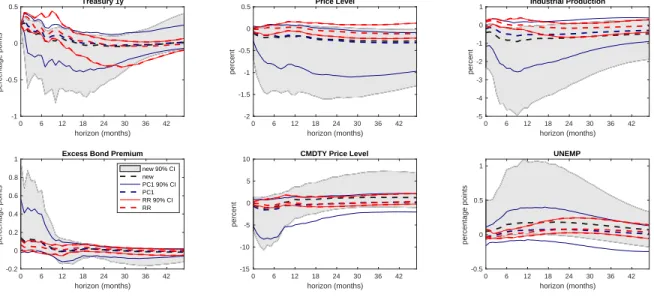
Figure 1.2 plots the impulse responses a monetary policy shock that on impact raises the one-year government bond yield by 25 basis points using the new measure, PC1 and Romer-Romer(RR) shock. The 90% confidence interval is constructed using the inference approach in Montiel Olea et al. (2018) for weak instrument.

Using the new measure, the estimates imply that a shock that raises the bond yield is contractionary: price level, commodity price level, industrial production drop immediately, excess bond premium and the unemployment rate increase. However, if we use the PC1, the effects on industrial production and unemployment rate never become significant, and the initial response of unemployment rate goes in the wrong direction; if we use Romer-Romer shock, the initial responses of both industrial production and the unemployment rate are inconsistent with the theory.

1.5

Conclusion

Evaluating the effects of monetary policy is important for both policy makers and researchers. In this paper, I provide a new method of constructing monetary policy shocks that can be used for monetary policy evaluation and compare it with the existing approaches. The new measure successfully isolates the non-information movement of the Federal Reserve’s announcement, whereas the previous methods are incapable to achieve. The new measure is consistent with the standard theory’s prediction: monetary policy shock is independent of recession period; a pure monetary policy tightening lowers private investors’ expectations about inflation and output growth; the majority of the comovement between S&P 500 futures and monetary policy shocks is negative. Furthermore, the new measure can be used as a relevant instrument for IV-SVAR analysis. “Price puzzle” and “Output puzzle” disappear in the analysis.

198801 199101 199401 199701 200001 200301 200601 200901 201201 201501 -1 -0.5 0 0.5 MP1 198801 199101 199401 199701 200001 200301 200601 200901 201201 201501 -1 -0.5 0 0.5 FF4 198801 199101 199401 199701 200001 200301 200601 200901 201201 201501-1 -0.5 0 0.5 PC1 198801 199101 199401 199701 200001 200301 200601 200901 201201 201501-2 -1 0 1 2 RR 198801 199101 199401 199701 200001 200301 200601 200901 201201 201501 -1 -0.5 0 0.5 MAR 198801 199101 199401 199701 200001 200301 200601 200901 201201 201501 -1 -0.5 0 0.5 NEW

Treasury 1y 0 6 12 18 24 30 36 42 horizon (months) -1 -0.5 0 0.5 percentage points Price Level 0 6 12 18 24 30 36 42 horizon (months) -2 -1.5 -1 -0.5 0 0.5 percent Industrial Production 0 6 12 18 24 30 36 42 horizon (months) -5 -4 -3 -2 -1 0 1 percent

Excess Bond Premium

0 6 12 18 24 30 36 42 horizon (months) -0.2 0 0.2 0.4 0.6 0.8 1 percentage points new 90% CI new PC1 90% CI PC1 RR 90% CI RR

CMDTY Price Level

0 6 12 18 24 30 36 42 horizon (months) -15 -10 -5 0 5 10 percent UNEMP 0 6 12 18 24 30 36 42 horizon (months) -0.5 0 0.5 1 percentage points

T able 1.1. Re gression on NBER Recession Indicator MP1 FF4 PC1 RR MAR NEW β -2.66*** -2.18*** -1.63** -0.18** -0.41 0.15 (0.85) (0.75) (0.67) (0.09) (1.02) (0.90) 1990:m1-2008:m12 1990:m1-2008:m12 1990:m1-2018:m12 1969:m3-2007:m12 1991:m1-2009:m12 1988:m1-2013:m12 NO TES: Rob ust standard errors are in parentheses, *, ** and *** denote statistical significance at 10 percent, 5 percent and 1 percent le v els, respecti v ely .

T able 1.2. Re gressions Estimating Pri v ate F orecast Responses to V arious Measures of Contractionary Moneta ry Polic y Shocks MP1 4 FF4 PC1 R R MAR NEW NEW (full sample) Inflation Current quarter 0.17 0.17 0.14 0.07 0.08 -0.03 0.06 (0.41) (0.32) (0.29) (0.07) (0.31) (0.32) (0.28) Ne xt quarter 0.10 0.11 -0.00 0.01 -0.09 -0.14 -0.06 (0.30) (0.22) (0.20) (0.05) (0.19) (0.18) (0.19) 2-quarter ahead -0.16 -0.15 -0.23 0.00 -0.37** -0.41** -0.21 (0.20) (0.15) (0.16) (0.05) (0.17) (0.19) (0.17) 3-quarter ahead 0.10 0.05 -0.06 -0.03 -0.18 -0.18 -0.13 (0.25) (0.18) (0.16) (0.04) (0.17) (0.17) (0.15) 4-quarter ahead -0.12 -0.09 -0.17 -0.00 -0.17 -0.24 -0.10 (0.22) (0.15) (0.15) (0.04) (0.16) (0.17) (0.15) Unemployment rate Current quarter -0.19 -0.15 -0.24** 0.02 -0.16 -0.08 0.04 (0.18) (0.13) (0.12) (0.04) (0.14) (0.13) (0.15) Ne xt quarter -0.18 -0.23 -0.21 0.02 -0.07 0.02 0.12 (0.23) (0.16) (0.14) (0.06) (0.16) (0.17) (0.20) 2-quarter ahead -0.31 -0.38** -0.29** 0.05 -0.16 -0.02 0.02 (0.28) (0.17) (0.14) (0.06) (0.17) (0.18) (0.23) 3-quarter ahead -0.31 -0.30* -0.24* 0.06 -0.06 0.05 0.14 (0.24) (0.16) (0.14) (0.05) (0.15) (0.16) (0.24) 4-quarter ahead -0.10 -0.16 -0.10 0.02 -0.01 0.05 0.36 (0.19) (0.14) (0.11) (0.06) (0.14) (0.15) (0.25)

Table 1.3.% of Days Where S&P 500 Moves in the Opposite Direction with Monetary Policy Shocks

Stock Market Index MP1 4FF4 PC1 RR MAR New New (full sample)

S&P 500 30-minute 51% 52% 71% 46% 64% 69% 68%

S&P 500 daily 45% 48% 57% 51% 56% 60% 58%

NOTES: This table displays % of days where S&P 500 moves in the opposite direction with non-zero monetary policy shocks. The sample period for the first six columns is from 1990:m1 to 2007:m12. The last column is from 1988:m1 to 2013:m12.

Chapter 2

Evaluating the Effects of Forward

Guid-ance and Large-scale Asset Purchases

Abstract

This paper evaluates the effects of forward guidance and large-scale asset purchases (LSAP) when the nominal interest rate reaches the zero lower bound. I investigate the effects of the two policies in a dynamic new Keynesian model with financial frictions adapted from Gertler and Karadi (2011, 2013), with changes implemented so that the framework delivers realistic predictions for the effects of each policy on the entire yield curve. I then match the change that the model predicts would arise from a linear combination of the two shocks with the observed change in the yield curve in a high-frequency window around Federal Reserve announcements, allowing me to identify the separate contributions of each shock to the effects of the announcement. My estimates correspond closely to narrative elements of the FOMC announcements. My estimates imply that forward guidance was more important in influencing inflation, while LSAP was more important in influencing output.

2.1

Introduction

Between December 2008 and December 2015, the federal funds rate - that is, the conventional monetary policy instrument of the Federal Reserve, or the Fed - consistently hovered near the zero lower bound (ZLB). To provide a much-needed stimulus to the economy,

the Federal Open Market Committee (FOMC) resorted to two unconventional monetary policies

at once: forward guidance and large-scale asset purchases (LSAP).1In this paper, I propose

a new method of separating the components of forward guidance and LSAP for each FOMC announcement, reconciling the various interest rates’ responses predicted from a structural model with observed high frequency yield curve data. In a follow-up step, I aggregate the effects from each type of monetary policy and provide quantitative estimates of the influence of each FOMC announcement on the financial market and the real economy.

The top reason for separating forward guidance from LSAP is that they affect the financial market and macroeconomy via different channels. When the Fed provides forward guidance - that is, communicating to the public about the likely future course of monetary policy - individuals

and businesses will use this information in making decisions about spending and investments.2

When the Fed purchases longer-term securities issued by the U.S. government and longer-term securities issued or guaranteed by government-sponsored agencies, long-term interest rates decline as risk premiums drop, which ultimately reduces the cost of borrowing for the private

sector.3 To better understand the efficacy of the policies and accurately estimate their effects,

however, we first need to quantify the importance of each type of monetary policy.

In this paper, I contribute to monetary policy evaluation literature in three ways: (i) by providing a micro-foundation of how various interest rates respond to different unconventional monetary policies, (ii) by quantifying the responses of financial markets and the real economy,

1_{For example, on December 16, 2008, the FOMC lowered the target for the federal funds rate to a range from 0}

to 1/4 percent and indicated that it expected the target to remain there “for some time”. In the same announcement,

the Fed announced that it would continue to consider ways of using its balance sheet to further support credit markets and economic activity.

2_{Eggertsson et al. (2003) show that lowering the expected path of policy rates can be highly effective in increasing}

economic activity and inflation for an economy at the zero lower bound. There is a rapidly growing literature on assessing the effect of forward guidance that has been used during the Great Recession. Important contributions include Campbell et al. (2012), Swanson and Williams (2014), Gertler and Karadi (2015), Del Negro et al. (2015), Keen et al. (2016) and Swanson (2017).

3_{Chen et al. (2012) augment a standard DSGE model with segmented bond markets, and Gertler and Karadi}

(2011, 2013) provide a framework where limits to arbitrage exist. Most empirical research has focused on analyzing the effects of LSAP on interest rates, output, inflation, term and risk in financial markets, and spillover effects in other countries. For example, Gagnon et al. (2011), Krishnamurthy et al. (2011), Gilchrist and Zakrajˇsek (2013), Bauer and Rudebusch (2014). Studies using a variety of methodologies generally agree that LSAP has been effective at lowering long-term interest rates and stimulating economic growth.

and (iii) by examining which type of unconventional monetary policy can more thoroughly explain those responses. To those ends, I develop a model that accounts for different channels of transmitting unconventional monetary policies and perform an empirical analysis using high-frequency interest rate data.

I begin by building a New Keynesian dynamic stochastic general equilibrium (DSGE) model based on the work of Gertler and Karadi (2011, 2013). I introduce a nominal short-term shadow interest rate that I assume follows a Taylor rule, as well as a forward guidance shock is the form of an announcement of future shocks to the interest rate rule, following the modeling device for generating innovations in expected future interest rates proposed by Las´een and Svensson (2011). I allow a ZLB where a one-period nominal interest rate endogenously remains when the economy enters a recession. Also following Gertler and Karadi (2011, 2013), I model LSAP as the central bank’s purchase of a perpetuity, which affects the economy to the extent that limits to arbitrage in private intermediation exist.

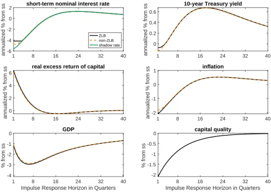
Next, I perform some model simulations in which the economy endogenously remains at the ZLB for a few periods as a result of a negative shock. I also suppose that either a forward guidance policy or an LSAP program involving the purchase of long-term securities is initiated in the wake of the shock. I obtain the different impulse responses of short-term shadow and perpetuity interest rates to each type of monetary policy.

The mechanisms by which the forward guidance and LSAP affect the shadow rate and the perpetuity rate differently are as follows. I assume that the central bank has limited commitment power and influences people’s expectations up to a finite horizon. That assumption is realistic insofar as the central bank wants to be flexible and adjust its monetary policy as economic conditions change. Instead of setting up an infinite horizon interest rate path now and changing it later, which will hurt its credibility, the central bank provides guidance for a short period. As a result, when the Fed exercises the forward guidance policy, the shadow interest drops below the perpetuity interest rate. When the Fed makes asset purchases, on the one hand it will increase the demand for the perpetuity interest rate and lower the long-term interest rate; on the other, it

will increase people’s expectations for short-term output and inflation, which will increase the shadow interest rate by way of the interest rate rule.

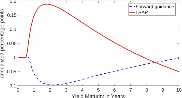
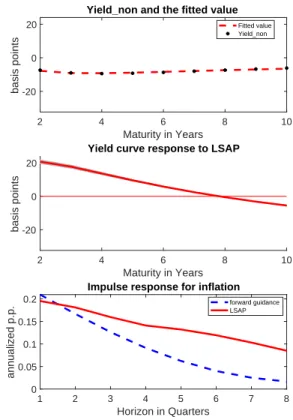
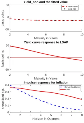
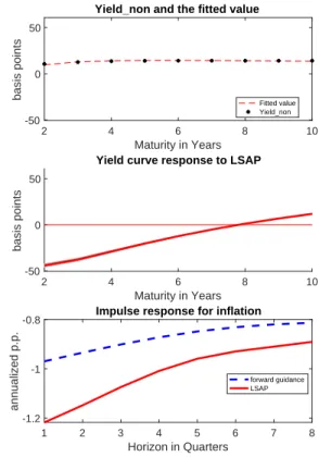
However, the daily change in the shadow rate cannot be observed in the data. To compare the model’s prediction with interest rate data, I thus interpolate the entire yield curve by using a two-factor yield curve interpolation method adapted from Wu and Xia (2016). As a result, forward guidance affects Treasury yields at all maturities, with a peak effect at a maturity of about 20 months. By contrast, the effects of LSAP increase along with maturity, meaning that LSAP exerts its peak effect on the longest-term maturities but increases short-term maturities.

One of the implications of using a formal model of LSAP such as the one developed here is that expansionary LSAP, by lowering long-term rates, stimulates the economy and helps achieve higher inflation and output at the intermediate run horizon. If the Fed in the future were to respond to the higher inflation and output with its usual Taylor rule, the result would be sooner lift-off from the zero lower bound and a higher path for short-term interest rates. The model predicts that LSAP would lower long-term interest rates but raise intermediate-term interest rates. If the Fed does not want to have this effect, it should always use expansionary forward guidance as a complementary tool in conjunction with LSAP. Our empirical estimates imply that this is typically what the Fed in fact did.

Next I combine the theoretical result with data to identify the sizes of forward guidance and LSAP for each Fed’s announcement. The data I use is the movements of Treasury yields at various horizons in a daily window that brackets the Fed’s announcement. Three forces drive those movements: the Fed’s superior information about economic conditions, the unexpected forward guidance policy, and the unexpected asset purchases policy. To isolate the latter two from the Fed’s information, I use Zhang (2018)’s method and regress the observed changes of yields at each maturity on the Green Book forecasts. The residuals are orthogonal to the Fed’s information and represent the monetary policy component of the Fed’s announcements. Then I match the change that the structural model predicts from a linear combination of the two types of shocks with this monetary policy component. Figure 2.1 shows the estimated size of each

type of monetary policy on each of the Fed’s announcement days.

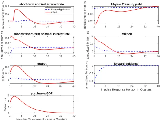
With the size of the policy shock at each date identified, I use the structural model to make inferences about the other variables of interest. Overall, my estimates indicate that the QE I program (i.e., from November 2008 to March 2010) increased two quarters ahead of real GDP by 1.11% and two quarters ahead of expected inflation by 0.81 annualized percentage points. Forward guidance thus exerts a greater influence on inflation expectations (0.60 vs. 0.21 annualized percentage points), whereas LSAP is more important in influencing output (0.39 vs. 0.72 percent).

This paper contributes to four major strands of literature on monetary policy evaluation. First, among economists who have increasingly emphasized the multidimensionality of monetary policy, Campbell et al. (2012) and Nakamura and Steinsson (2018) have found that the Fed’s announcements contain information about economic conditions. However, to the best of my knowledge, only Swanson (2017), who mobilized principal component representations of various interest rates, has separated the effects of forward guidance and LSAP for each of the Fed’s announcements. My paper differs from Swanson’s (2017) work in three aspects. (i) I decompose the movement in various interest rates into information effects and monetary policy effects, the latter of which I decompose into forward guidance and LSAP. Crucially, that separation directs my estimates to show that much of the movement in interest rates results from the Fed’s information; without that distinction, by contrast, the overall effects on real GDP are three times larger. (ii) My paper provides a micro-foundation of the different effects of forward guidance and LSAP on the yield curve. (iii) My method can allow practitioners and researchers to forecast the long-term effects on real activity by using a structural model; otherwise, by using time series approach, such forecasting is quite difficult to achieve, because the sample period for ZLB only lasted for 7 years.

The second strand of literature to which my paper contributes is the use of event studies such as Gagnon et al. (2011), Krishnamurthy et al. (2011), for instance - to assess the effects of

four unconventional monetary policies on interest rates.4 Instead of using text analysis to discern changes in words and sentences in current FOMC statements compared to previous statements or whether the event date belongs to a certain period of policy implementation, I allow the data indicate the direction and size of monetary policy. Using this approach can capture anything the Fed does or fails to do that affects the market. For example, if the Fed chose not to take some

action or not to make a change in wording that the market anticipated5, that absence of action

can also be interpreted as revealing new information about monetary policy to the market. Third, my paper provides a micro-foundation for identifying assumptions made in empirical studies. Gertler and Karadi (2015), for instance, have used external instruments in a vector autoregression (VAR) to identify monetary policy shocks and 1- and 2-year Treasury bond yields as conceptually preferred policy indicators to study the mechanism of the transmission of forward guidance. Earlier, Chung et al. (2012) estimated a structural model that assumes that the term premium of long-term Treasury bonds is inversely proportional to the Fed’s holdings of long-term securities. The following year, Baumeister and Benati (2013) employed a time-varying parameter structural VAR model under the assumption that LSAP lowers the long-term yield spread while short-term interest rates remain unchanged.

Fourth and last, my paper draws from empirical studies on channels used to signal the Fed’s bond purchases. Previously, scholars such as Bauer and Rudebusch (2014) found that such purchases have important signaling effects that lower expected future short-term interest rates by

using an event study. My paper provides a theoretical explanation for their finding6: a LSAP

announcement that causes output and inflation to rise today implies higher interest rates today,

4_{Wright (2012) uses a structural VAR to identify the effects of monetary policy shocks on various long-term}

interest rates. The VAR is identified using the assumption that monetary policy shocks are heteroskedastic: monetary policy shocks have higher variance on days of FOMC meetings and certain speeches than the other days.

5_{For example, on January 28, 2009, the FOMC statement was interpreted by some market participants as}

disappointing because of its lack of concrete language regarding the possibility and timing of purchases of longer-term Treasuries in the secondary market contrary to the other announcements Gilchrist and Zakrajˇsek (2013); Bauer and Rudebusch (2014). As another example, on September 18, 2013, the FOMC was widely expected to begin tapering its asset purchase while it turned out not to do so.

6_{Bhattarai et al. (2015) build a signaling theory where QE is effective because it generates a credible signal of}

particularly via the endogenous component in the central bank’s policy rule. Therefore, to keep short-term rates at a low level, an additional expansionary policy should be implemented.

The remainder of the paper proceeds as follows. In Section 2.2, I begin by describing the model, which I calibrate in Section 2.3 to match the key features of the data, as well as calculate the state-dependent impulse responses in different scenarios. In Section 2.4, I describe the shadow interest rate framework used, after which I describe the regression methodology and results in Section 2.5. In Section 2.6, I discusses the key announcement days, and I explain the robustness of my methodology in Section 2.7. Last, I close the paper in Section 3.4 by summarizing the findings.

2.2

A Structural Model

My framework is based on the model of Gertler and Karadi (2011, 2013). They modify a reasonably standard New Keynesian model to explicitly include financial market structure and financial balance sheets. The model makes three primary assumptions. Banks finance risky, long-term assets with riskless, short-term debt. The existence of an agency problem between households and banks constrains the borrowing ability of the latter and generates excess return between long- and short-term debts. The central bank provides mediation for long-term asset purchases during economic crises and boosts the economy by reducing the credit costs of the banking sector.

I add the following features to their model. First, I introduce a nominal short-term shadow interest rate that I assume follows a Taylor rule subject to the ZLB. The shadow interest rate is the short-term rate when the ZLB is not binding. The shadow rate is negative when the ZLB is binding. A larger negative value implies a longer period of time before the shadow rate becomes positive and there is a lift-off from the ZLB. Downward shocks to the shadow rate can thus be used as a way to represent forward guidance in the ZLB. Instead of assuming that the one-period nominal interest rate is pegged for a certain length of time as in Gertler and Karadi, in my model

the length of time that the economy stays at the ZLB is an endogenous response to the interaction between forward guidance and other shocks.

In the following part of this section, I characterize the distinctive elements of the model, including the behavior of households, banks, producers, and the central bank. See Online

Appendix7for thorough expositions of the model.

2.2.1

Households

The economy is populated by a continuum of households of measure unity. Within

each household there are two types of members: workers and bankers. A fraction 1−f of

the household members are workers, and a fraction f are bankers. Workers provide labor and

earn wages. Each banker manages a financial intermediary and returns the profit back to the household. Within the family there is perfect consumption insurance.

A banker this period remains a banker next period with probability θ, implying the

average survival time for a banker in any given period is 1/(1−θ). After the bankers exit, their

retained earnings return to their respective household in the form of dividends. The bankers who exit become workers and are replaced by a similar number of workers randomly; thus the relative

proportion of each type is fixed. New bankers will get startup funds equal toX_t provided by the

household.

Letc_t be consumption andl_tlabor supply. Then the household’s discounted utilityu_t is

given by: ut=Et ∞

∑

where β ∈(0,1) denotes the household’s subjective discount factor, h∈ (0,1) governs the

strength of habits, andχ,φ >0. The household’s inter-temporal elasticity of substitution is unity,

and its Frisch elasticity of labor supply is 1/φ.

7_{The Online Appendix can be found at http://acsweb.ucsd.edu/}∼_{xuz039/pdfs/JobMarketPaperAppendix}

There are three types of assets that the household can hold. Households can borrow and

lend in a default-free one-period nominal bond market at the nominal interest rateit. Subject to

some transaction costs, they can also make private loans to non-financial firms to finance capital

to earn the real rate of returnR_kt and hold a nominal long-term government bond to earn the real

rate of returnR_bt.

LetS_ht be the amount of private securities that households have. The transaction cost is

equal to the percentage 1₂κs(Sht−Sh)2/Sht of the value of the securities in its respective portfolio

forS_ht >S_h. Similarly, for government bonds there is a holding cost equal to the percentage

1

2κb(Bht−Bh) 2_/B

ht of the total value of government bonds held forBht >Bh, whereBht is the

amount of long-term government bond that households have.

I defineP_t as the price level of the consumption good. Q_t is the real price of the private securities at timet, andq_tbe the real price of the government bond at timet.

Accordingly, at timetthe household faces a flow budget constraint in nominal term:

P_tc_t+P_tD_ht+P_tQ_t[S_ht+1 2κs(Sht−Sh) 2_{] +P} tqt[Bht+ 1 2κb(Bht−Bh) 2_{] +P} tTt+PtXt =PtWtlt+PtΠt+ (1+it−1)Pt−1Dht−1+Pt−1RktQt−1Sht−1+Pt−1Rbtqt−1Bht−1. (2.2)

where D_ht is the quantity of one-period nominal bond held by household at timet, Tt is the

lump-sum taxes in real term,Xt is the total transfer the household gives to its members that enter

banking att,Wt is the real wage, and Πt are the payouts to the household from ownership of

both non-financial and financial firms in real term.

to (2.2). The first-order conditions are: ∂ut ∂ct W_t = χl_tφ EtΛt,t+1Rt = 1 S_ht−S_h = 1 κs EtΛt,t+1(Rkt+1−Rt) B_ht−B_h = 1 κ_bEtΛt,t+1(Rbt+1−Rt)

where the household’s stochastic discount factor isΛt,t+1≡β ∂ut/∂ct

∂ut/∂ct+1.

Letπt≡ _PtP₋t₁−1 be the inflation rate, then the link between nominal interest rateit and

real interest rateRt is given by the Fisher equation:

1+i_t=R_t(1+Etπt+1)

Following Woodford (2001) and other authors (e.g Arellano and Ramanarayanan (2012), Chen et al. (2012)), I model the nominal long-term government bond as a depreciating nominal perpetuity that pays a geometrically declining coupon ofϑndollars in each periodn=1,2, . . .

after issuance. Letq_tn≡P_tq_t be the nominal price of the nominal bond. Then the ex-coupon real

rate of return on the nominal bondR_bt is given by

R_bt = 1/Pt+ϑqt

q_t−1 =

1+ϑqn_t

qn_t−1(1+πt)

where the size of the next coupon payment is normalized to one dollar. The very simple recursive structure above makes this type of long-term bond extremely convenient to work

with. By choosing ϑ appropriately, we match the perpetuity’s Macauley duration with the

2.2.2

Banks

Banks lend funds obtained from households to non-financial firms and to the government. In addition to acting as specialists that assist in channeling funds from savers to investors, they engage in maturity transformation. They hold long-term assets and fund these assets with short-term liabilities (beyond their own equity capital). Financial intermediaries in this model are meant to capture the entire banking sector, i.e., investment banks as well as commercial banks. Letn_t be the amount of net worth that a banker/intermediary has at the end of periodt,d_t

the deposits the intermediary obtains from households,s_pt the quantity of financial claims on

non-financial firms that the intermediary holds, andb_t the quantity of long-term government

bonds. The intermediary balance sheet is then given by:

Qtspt+qtnbpt =nt+dt (2.3)

Net worth is accumulated through retained earnings. It is thus the difference between the gross return on assets and the cost of liabilities:

nt=RktQt−1spt−1+Rbtqtn−1bpt−1−Rt−1dt (2.4)

The banker’s objective is to maximize the discounted stream of payouts back to the household, where the relevant discount rate is the household’s inter-temporal marginal rate of substitution. The terminal wealth is given by:

Vt =Et

∞

∑

i=1

(1−θ)θi−1Λt,t+int+i (2.5)

To motivate a limit on the bank’s ability to obtain deposits, Gertler and Karadi (2011) introduce a moral hazard/costly enforcement problem. At the beginning of the period, the banker can choose to divert funds from the assets he holds and transfer the proceeds to the household of

which he is a member. The cost to the banker is that the depositors can force the intermediary into bankruptcy and recover the remaining fraction of assets. However, it is too costly for the depositors to recover the funds that the banker diverted. It is assumed that it is easier for the bank to divert funds from its holdings of private loans than from its holding of government bonds: it can divert the fractionλ of its private loan portfolio and the fractionλ4with 0<4<1 from

its government bond portfolio. Therefore, for depositors to be willing to supply funds to the banker, the following incentive constraint must be satisfied:

Vt ≥λQtspt+λ4qn_tbpt (2.6)

The left side is what the banker would lose by diverting a fraction of assets. The right side is the gain from doing so. The banker’s maximization problem is to chooses_t,b_t, andd_t to

maximize (2.5) subject to (2.3), (2.4), and (2.6). LetΓt be the Lagrange multiplier associated

with the incentive constraint. The first order conditions are:

EtΛe_t,t+1(R_kt+1−R_t) = Γt 1+Γt λ EtΛe_t,t+1(Rbt+1−Rt) =4 Γt 1+Γt λ with e Λt,t+1 ≡ Λt,t+1Ωt+1 Ωt = 1−θ+θ ∂Vt ∂nt ∂Vt ∂nt = Λe_t−1,t[(Rkt−Rt−1)φt+Rt−1]

The constraints are: Q_ts_pt+4qn_tb_t =φtnt if Γt >0 <φtnt if Γt =0 where φt = EtΛe_t,t+1R_t λ−EtΛe_t,t+1(R_kt+1−R_t)

2.2.3

Central bank’s asset purchases

The central bank is allowed to purchase quantities of private loansS_gt and long-term

government bondsB_gt. To finance these purchases, it issues risk-free short-term debtD_gt that

pays the safe market interest ratei_t. In particular, the central bank’s balance sheet is given by

QtSgt+qtBgt=Dgt.

When limits to arbitrage in the private market are operative, the central bank’s acquisition of securities will have the effect of bidding up the prices on each of these instruments and down the excess returns.

2.2.4

Aggregation

LetS_pt be the total quantity of loans that banks intermediate, B_pt the total number of

government bonds they hold, and N_t their total net worth. Since neither component of the

maximum adjusted leverage ratio depends on bank-specific factors, we can simply sum across the portfolio restriction on each individual bank to obtain

Total net worth evolves as the sum of the retained earnings by the fractionθ of surviving

bankers and the transfers that new bankers receive, X, as follows:

Nt =θ[(Rkt−Rt−1)

Q_t−1S_pt−1

N_t−1 + (Rbt−Rt−1)

qn_t−1B_pt−1

N_t−1 +Rt−1]Nt−1+Xt

Let S_t and B_t be the total supplies of private loans and long-term government bonds,

respectively. Then by definition,

St = Spt+Sht+Sgt

B_t = B_pt+B_ht+B_gt

We combine these identities with the balance constraint on the banks to obtain the following relation for the total value of private securities intermediated:

Q_t(S_t−S_ht−S_gt)≤φtNt− 4qtn[Bt−(Bgt+Bht)] (2.7)

2.2.5

The Production Sector

Intermediate goods firms

The economy also contains a continuum of infintely-lived monopolistically competitive firms, each producing a single differentiated good. Each operates a constant returns to scale technology with capital and labor inputs and have identical Cobb-Douglas production functions:

Y_t=A_t(ξtKt−1)αlt1−α

whereξt is a random disturbance that we refer to as a “capital quality” shock. The capital quality

shock as a simple way to introduce an exogenous source of variation in the return to capital. It is best thought of as capturing some form of economic obsolescence, as opposed to physical depreciation.