Financial Globalization, Financial Crises and Contagion

(1)

NBER WORKING PAPER SERIES

FINANCIAL GLOBALIZATION, FINANCIAL CRISES AND CONTAGION

Enrique G. Mendoza

Vincenzo Quadrini

Working Paper 15432

http://www.nber.org/papers/w15432

NATIONAL BUREAU OF ECONOMIC RESEARCH

1050 Massachusetts Avenue

Cambridge, MA 02138

October 2009

This paper was prepared for the Carnegie-Rochester Conference on Public Policy held April 17-18,

2009 at the University of Rochester. We would like to thank Gian Luca Clementi for discussing the

paper and providing us with insightful comments. We also thank conference participants, as well as

Frank Warnock and Luis Cespedes, for their comments and suggestions. Financial support from the

National Science Foundation is gratefully acknowledged. The views expressed herein are those of

the author(s) and do not necessarily reflect the views of the National Bureau of Economic Research.

NBER working papers are circulated for discussion and comment purposes. They have not been

peer-reviewed or been subject to the review by the NBER Board of Directors that accompanies official

NBER publications.

© 2009 by Enrique G. Mendoza and Vincenzo Quadrini. All rights reserved. Short sections of text,

not to exceed two paragraphs, may be quoted without explicit permission provided that full credit,

(2)

Financial Globalization, Financial Crises and Contagion

Enrique G. Mendoza and Vincenzo Quadrini

NBER Working Paper No. 15432

October 2009

JEL No. E44,F36,F41

ABSTRACT

Two observations suggest that financial globalization played an important role in the recent financial

crisis. First, more than half of the rise in net borrowing of the U.S. nonfinancial sectors since the mid

1980s has been financed by foreign lending. Second, the collapse of the U.S. housing and

mortgage-backed-securities

markets had worldwide effects on financial institutions and asset markets. Using an

open-economy

model where financial intermediaries play a central role, we show that financial

integration

leads to

a sharp rise in net credit in the most financially developed country and leads to large asset price

spillovers

of country-specific shocks to bank capital. The impact of these shocks on asset prices are

amplified

by bank capital requirements based on mark-to-market.

Enrique G. Mendoza

Department of Economics

University of Maryland

College Park, MD 20742

and NBER

[email protected]

Vincenzo Quadrini

Department of Finance and Business Economics

Marshall School of Business

University of Southern California

701 Exposition Boulevard

Los Angeles, CA 90089

and NBER

(3)

1 Introduction

The global financial crisis that started with the meltdown of the U.S.

sub-prime mortgage market in 2007 was preceded by a twenty-year period of

substantial growth in debt and leverages, in an environment of increasing

world financial integration, low real interest rates and growing U.S. external

deficits. During this period of widening “global imbalances” we also observed

several financial crises in emerging economies with cross-country contagion

that in some cases did not appear driven by fundamentals. Some of these

crises affected the capital markets of the industrial world (particularly the

LTCM crisis in the aftermath of the 1998 Russian crash).

These events have generated a large body of research with well-established

contributions. Until now, however, the study of global imbalances and the

study of financial crises and contagion have remained somewhat separate

sub-jects. In contrast, this paper addresses the question of whether the ongoing

global financial crisis and the process of financial globalization are related. In

particular, we study two issues. First, whether financial globalization

con-tributed to the buildup of high leverages in some industrialized countries,

especially the U.S. Second, whether credit frictions amplify the effects of

shocks to the balance sheet of banks and how these effects are transmitted

across countries.

The motivation for this paper derives from the evidence provided in Figure

1 according to which the U.S. credit boom was largely fueled by foreign

lending.

1. The first panel of Figure 1 shows that the net debt-income ratio of the

U.S. nonfinancial sectors doubled between 1982 and 2008 (net credit

market assets as a ratio of GDP of these sectors fell from -1 to about

-2). A surge in net debt of this magnitude, which affected all three

nonfinancial sectors (households, nonfinancial businesses, and the

gov-ernment), is unprecedented in the data available since 1946.

1

2. Starting in the mid 1980s, the integration of world capital markets that

resulted from the removal of capital controls and innovations in

finan-cial markets produced significant changes in gross and net foreign asset

1_{Data is from the Flow of Funds of the Federal Reserve Board. Net credit is defined}

as credit market assets minus credit market liabilities. Credit market assets and liabilities exclude all non-debt financial instruments, particularly equity holdings.

(4)

Figure 1: Net credit before and after financial integration.

1.0 1.5 2.0 2.5

U.S. Net Credit Market Assets as a Share of GDP Domestic nonfinancial sector

Financial sector Rest of the world

‐2.0 ‐1.5 ‐1.0 ‐0.5 0.0 0.5 1946 1951 1956 1961 1966 1971 1976 1981 1986 1991 1996 2001 2006

Foreign credit market borrowing and lending

(fraction of GDP) 0.5 0.6 Foreign borrowing Foreign lending 0.4 0.3 0.2 0.1 0 1960 1965 1970 1975 1980 1985 1990 1995 2000 2005 0.6

Ratio of Net U.S. Assets Held by Rest of the World to Net U.S. Assets of the Domestic Nonfinancial Sector net credit market debt

0.5

net credit market debt net total financial assets U.S. Treasuries 0.3 0.4 0.2 0.1 ‐0.1 0.0 1946 1951 1956 1961 1966 1971 1976 1981 1986 1991 1996 2001 2006

(5)

positions worldwide (see Lane & Milesi-Ferretti (2006)). In the United

States, both gross and net foreign borrowing rose sharply. Regarding

net foreign credit, about half of the increase in the net debt-income

ratio of the nonfinancial sectors mentioned above was financed by a

rise in net credit assets held by the rest of the world (see again the top

panel of Figure 1), and this was also an unprecedented phenomenon

in the post-war period. Before the mid 1980s, the U.S. fitted well the

definition of financial autarky: The net debt of the domestic

nonfinan-cial sectors was almost identical to the net credit assets of the finannonfinan-cial

sector, with a zero net credit position for the rest of the world.

2

_In

terms of gross positions, the second panel of Figure 1 shows that the

foreign credit claims on U.S. nonfinancial sectors grew sharply since

1985, while U.S. lending to foreigners (i.e. claims of the U.S.

nonfinan-cial sectors on foreign agents) experienced a relatively modest increase.

As a result, net credit assets held by the rest of the world vis-a-vis the

United States grew by 50 percentage points of U.S. GDP since 1982.

3. The above trends identified in net credit assets are even more

pro-nounced for net total financial assets and net Treasury securities, as

shown in the bottom panel of Figure 1. The plot shows the net asset

positions of the U.S. vis-a-vis the rest of the world as a ratio of the

corresponding net asset positions held by the domestic nonfinancial

sectors for three asset categories: credit market assets (as in the top

two panels), total financial assets (which include non-credit assets like

equity), and U.S. Treasury bills. The ratios for credit assets and total

financial assets hover near zero before the mid 1980s, reflecting again

the fact that before financial globalization the U.S. was effectively in

financial autarky. By the end of 2008, however, net credit assets held

by the rest of the world amounted to 1/5 of U.S. net credit liabilities

of the nonfinancial sectors, and for total financial assets the ratio was

even higher at about 1/3. For T-bills, the rest of the world increased

its positive net position sharply with the collapse of the Bretton Woods

system in the early 1970s, but even that increase dwarfs in comparison

2_{Note that the data for financial sectors combines domestic and international}

compo-nents, and hence it is not accurate to associate the financial sectors data with domestic financial sectors. Before financial integration, the international components were negligi-ble, so the association was valid. After the mid 1980s, however, part of the rise in net credit of financial sectors reflects also the effects of financial globalization.

(6)

with the surge observed since the mid 1980s. By 2008, the rest of the

world was a net holder of about one in every two T-bills held outside

of the U.S. financial sectors.

The fact that a large fraction of the credit expansion experienced by the

U.S. economy was financed by foreign borrowing raises several questions.

First, was the surge in debt in the United States a consequence of financial

globalization? Second, if globalization led to higher U.S. leverages, did the

higher leverages make the current crisis worse for asset prices? Third, did

globalization strengthen the spillover effects of the crisis to other countries?

In order to address these issues, we start with a model that can

ratio-nalize both the expansion in domestic credit within the United States and

the growth of its liabilities, vis-a-vis the rest of the world, following

finan-cial integration. The model extends the framework of Mendoza, Quadrini,

& R´ıos-Rull (2009) which has proven useful for explaining these two features

of the data. This new setup, however, differs in two important dimensions.

The first difference is that the model features three sets of economic agents

within each country: savers (or wage earners), producers (or capital owners),

and financial intermediaries. In Mendoza et al. (2009) savers and producers

were merged in a single agent and financial intermediaries were not explicitly

modeled. As we will see, the intermediation sector plays a central role in

the analysis of the current paper. The second difference is that the analysis

conducted in Mendoza et al. (2009) is limited to steady states and

transi-tions from a steady state with financial autarky to one with full financial

integration. In this paper, instead, we focus on the effects of unanticipated

(and hence non-diversifiable) shocks that hit the net worth of financial

inter-mediaries.

In our model, savers receive endowment incomes that are subject to

id-iosyncratic shocks. They can trade state-contingent claims with financial

intermediaries but there are constraints to the set of feasible claims. These

constraints derive from incentive-compatibility conditions imposed by limited

enforceability of financial contracts, which differs across countries. Countries

with higher enforcement systems allow for better insurance of the

idiosyn-cratic risks and lower propensity to save. As a result, these countries tend

to accumulate negative net foreign asset positions.

Producers do not face idiosyncratic uncertainty, so effectively we assume

a representative producer.

They also trade with financial intermediaries

(7)

and face limited enforcement of contracts, which takes the form of a

collat-eral constraint. Financial intermediaries raise funds from savers with

state-contingent deposits and make loans to producers. They own a fixed amount

of physical capital and face a capital requirement that affects their ability

to intermediate funds from savers to producers. The capital requirement

is linked to the equity of the intermediaries valued at market prices (as in

mark-to-market accounting). The structure of the intermediation sector has

some similarities with Van-denHeuvel (2008).

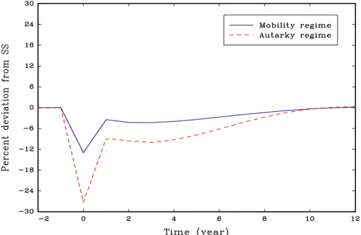
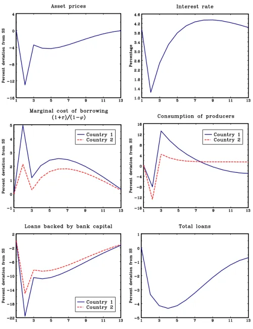
The main simulation exercise we conduct in the paper consists in a ‘small’

unanticipated shock that reduces the value of banks’ equity (by about 0.5

percent the value of world wide loans). This unanticipated shock induces a

large reduction in asset prices (almost 13 percent on impact). Moreover, it

takes a long period of time for asset prices to fully recover (about 12 years).

Since in a financially integrated economy asset prices are global, this price

decline is the vehicle for international contagion of the financial crisis. Asset

price declines are smaller than they would be in the presence of the same

shock under financial autarky. This is precisely because the shock affects the

asset prices worldwide, and not just the country where the shock originated.

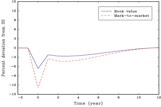
We then examine the quantitative effects of shifting from a capital

require-ment based on mark-to-market to a system based on historical prices. The

role played by mark-to-market accounting in the recent financial crisis has

been widely debated. Because of this accounting principle, the recent asset

price drop has caused a large decline in the equity value of banks, impairing

their ability to make loans. This has led many academics and practitioners to

propose the suspension or adjustment of this principle given the widespread

financial difficulties (see, for example, the interviews with Robert Shiller and

James Chanos in the March 30, 2009 Wall Street Journal). Our results

in-dicate that, if the mark-to-market accounting was replaced with a system

based on historical prices, the response of asset prices to shocks affecting the

balance sheet of banks would be significantly smaller.

The financial mechanisms at work in our model are related to several

mechanisms studied in the literature on ‘credit channels’ and ‘financial

ac-celerators’. Classic references include Fisher (1933), Bernanke & Gertler

(1989) and Kiyotaki & Moore (1997). Meh & Moran (2008) extended this

class of models to an environment where bank capital plays a central role

in the transmission of monetary shocks. Gertler & Karadi (2009)

exam-ined the effects of government credit provision to distressed banks. Aguiar

& Drumond (2007), Drumond & Jorge (2008), Van-denHeuvel (2008) and

(8)

Zhu (2007) also use models where the behavior of financial intermediaries

is important for macroeconomic fluctuations. Similar mechanisms, although

without an explicit modeling of the banking sector, have been used to study

Sudden Stops and financial contagion in emerging economies during the 1990s

(see, for example, Caballero & Krishnamurthy (2001), Calvo (1998), Cook &

Devereux (2006), Gertler, Gilchrist, & Natalucci (2007), Mendoza & Smith

(2006), Mendoza (2008) and Paasche (2001)). Our work is also related to

the recent studies examining the implications of financial integration among

countries that are heterogenous in the degree of domestic financial

develop-ment (see Aoki, Benigno, & Kiyotaki (2007), Caballero, Farhi, & Gourinchas

(2008), Mendoza, Quadrini, & R´ıos-Rull (2008), Mendoza et al. (2009) and

Prades & Rabitsch (2007)).

The rest of the paper is organized as follows. Section 2 describes the

struc-ture of the model. Section 3 explores the properties of the model numerically.

Section 4 examines the implications of changing the mark-to-market rule and

Section 5 conducts a sensitivity analysis. The final Section 6 concludes.

2 Analytical Framework

We extend the model studied in Mendoza et al. (2009) by adding a more

structured financial intermediation sector. The goal is to study how the

behavior of financial intermediaries in response to shocks to their balance

sheet propagate these shocks to the rest of the economy.

There are two countries, indexed by

i

∈ {

1 ,

2 }

, each inhabited by a

con-tinuum of agents of total mass

µ

i

. Agents are of two types: producers and

savers, each of mass

µ

i

/

2. They all have the same preferences and maximize

the lifetime utility

E

P∞

t=0

β

t

U

(

c

t

), where

c

t

is consumption at time

t

and

β

is

the intertemporal discount factor. The utility function is strictly increasing

and concave with

U

(0) =

−∞

and

U

000

(

c

)

>

0. Each country is endowed with a fixed per-capita supply ¯

k

of a

non-reproducible, internationally immobile asset, traded at price

P

_ti

. This asset is

used in production as specified below. We now describe the specific aspects

of the two types of agents.

2.1 Savers

Savers are very similar to the agents described in Mendoza et al. (2009)

ex-cept that they do not have the managerial ability to generate income through

(9)

the use of the productive asset. They receive income in the form of an

id-iosyncratic

stochastic endowment

w

t

, with a Markov conditional probability

distribution denoted by

g

(

w

t

, w

t+1

). We also assume that the savers are

the shareholders of the financial intermediaries from which they receive

non-negative dividends

d

t

.

Savers can buy contingent claims,

b

(

w

t+1

), that depend on the next

pe-riod’s realizations of the endowment. In absence of aggregate uncertainty,

the price of one unit of consumption goods contingent on the realization of

w

t+1

is

q

ti

(

w

t

, w

t+1

) =

g

(

w

t

, w

t+1

)

/

(1 +

r

ti

), where

r

it

is the equilibrium interest

rate.

3

_{The budget constraint for an individual saver is:}

d

t

+

w

t

+

b

(

w

t

) =

c

t

+

X

wt+1

b

(

w

t+1

)

q

ti

(

w

t

, w

t+1

)

.

(1)

Market incompleteness on the side of savers is modeled by assuming

lim-ited enforcement. Contracts are not perfectly enforceable due to the limlim-ited

(legal) verifiability of shocks. Because of this, savers can divert part of their

endowment but they lose a fraction

φ

i

of the diverted income. The parameter

φ

i

_{characterizes the degree of enforcement of financial contracts in country}

i

. Appendix A shows that, under the assumptions that agents cannot be

excluded from financial markets and there is limited liability, incentive

com-patibility imposes the following two constraints:

b

(

w

1

)

−

b

(

w

j

)

≤

φ

i

· w

j

−

w

1

(2)

w

j

+

b

(

w

j

)

≥

0 (3)

for all

j

∈ {

1 , ..., J

}

. Here

J

denotes the number of all possible realizations

of the endowment and

w

1

is the lowest (worst) realization.

The first condition requires that insurance received through contingent

claims,

b

(

w

1

)

−

b

(

w

j

), cannot be bigger than the variation in income, scaled

by

φ

i

_{. When}

_φ

i

_{is sufficiently large, savers are able to get full insurance of}

idiosyncratic risk and maintain constant consumption. When

φ

i

_{= 0, only}

non-state-contingent claims are feasible. A key assumption is that

φ

i

per-tains to the country of residency of the savers. Cross-country differences in

financial development are captured by differences in

φ

i

_{. The second}

con-straint derives from limited liability. The assumption is that a saver can

3_{The contingent claims are sold by competitive intermediaries as described below.}

(10)

always default on a contract at the beginning of next period. At this point

the intermediary can only recover the endowment

w

j

.

Let

{

q

_τi

(

w

τ

, w

τ+1

)

}

∞τ=t

be a (deterministic) sequence of prices in country

i

. The optimization problem of an individual saver can be written as:

V

_ti

(

w, b

) =

max

c, b(w0₎ (

U

(

c

) +

β

X w0

V

_ti₊₁

w

0

, b

(

w

0

)

g

(

w, w

0

)

(4)

subject to

(1)

,

(2) and (3)

The solution to the saver’s problem yields decision rules for consumption,

c

i

t

(

w, b

), and contingent claims,

b

it

(

w, b, w

0

_{). The decision rules determine}

the evolution of the distribution of savers over

w

and

b

. The distribution is

denoted by

M

_ti

(

w, b

).

We show in Appendix B that, by properly redefining the stochastic

pro-cess for the endowments, the problem can be reformulated as if each saver

chooses non-contingent claims, that is,

V

_ti

( ˜

w,

¯

b

) =

max

c,¯b0_≥−_w1_˜ (

U

(

c

) +

β

X w0

V

_ti₊₁

w

˜

0

,

b

¯

0

g

( ˜

w,

w

˜

0

)

(5)

subject to

d

+ ˜

w

+ ¯

b

=

c

+

¯

_b

0

1 +

r

i t

where ˜

w

is a transformation of

w

derived in the appendix and ¯

b

is the expected

value of the contingent claims. The solution can then be characterized by

the first order condition:

U

0

(

c

t

)

≥

β

(1 +

r

ti

)

EU

0

(

c

t+1

)

(6)

which is satisfied with equality if ¯

b

0

>

−

w

˜

1

.

2.2 Producers

Differently from Mendoza et al. (2009), we assume that the owners and

users of the productive asset—the producers—are different from other agents

(11)

(savers). This separation makes the model more tractable when we consider

unanticipated financial shocks.

Producers receive a constant flow of endowment

w

p

and generate income

y

t+1

=

F

(

k

t+1

) =

Ak

tν+1

, where

k

t+1

is the quantity of the productive asset

purchased at time

t

. The parameter

ν

is smaller than 1 because of limited

managerial capital that each producer has. Managerial capital is

interna-tionally mobile. Therefore, with capital mobility producers can choose to

operate at home, buying the domestic productive asset, or abroad, buying

the foreign productive asset. But they cannot do both. To keep the problem

simple we have deliberately assumed that producers do not face idiosyncratic

uncertainty neither in the endowment

w

p

_{nor in production. Therefore, we}

can focus on the representative producer.

As in the case of savers, producers can enter in contractual arrangements

with financial intermediaries. Because producers do not face idiosyncratic

uncertainty, their financial contracts are not state contingent. Denote by

l

t+1

/

(1 +

r

ti

) the loan contracted with a financial intermediary. In addition

to the interest rate, the bank also charges a financial cost

ϕ

i

t

(

l

t+1

) which is

nonnegative, increasing and convex in the loan size. Therefore, the producer

receives the funds [

l

t+1

−

ϕ

it

(

l

t+1

)]

/

(1 +

r

ti

) at time

t

and promises to repay

l

t+1

at

t

+ 1. The precise nature of this cost will be specified later in the

description of the banking sector. We anticipate here that this cost will be

zero at steady state and it plays a role only in equilibria in which the equities

of the financial intermediaries are low.

Limited enforcement constrains the amount that the intermediary is

will-ing to lend as follows:

l

t+1

≤

ψ

i

·

h

k

t+1

P

ti+1

+

F

(

k

t+1

)

i

(7)

This constraint derives from the assumption that the producer can always

default on a contract at the beginning of next period. At this point the

intermediary can only recover a fraction

ψ

i

of the producer’s assets, that is,

the market value of productive capital plus production. The parameter

ψ

i

could differ across countries which justifies the superscript

i

.

4

The producer starts the period with capital

k

t

and liabilities

l

t

and solves

4_{As we will see, the equilibrium interest rate is usually lower than the intertemporal}

discount rate due to the precautionary motive of savers. Because of this, producers have an incentive to borrow as much as possible. The above enforcement constraint makes sure that borrowing is bounded.

(12)

the following problem:

W

_ti

(

k, l

) = max

c,k0_,l0 (

U

(

c

) +

βW

_ti₊₁

k

0

, l

0 )

(8)

subject to

w

p

+

kP

_ti

+

F

(

k

) +

l

0

₋

_ϕ

i t

(

l

0

₎

1 +

r

i t

=

c

+

l

+

k

0

l

0

≤

ψ

ih

k

0

P

_ti₊₁

+

F

(

k

0

)

i

which is subject to the budget and enforcement constraints.

Given a deterministic sequence of prices

{

r

i_τ

, P

_τi

, ϕ

i_τ

(

.

)

}

∞

τ=t

, the solution is

characterized by the following first order conditions:

U

0

(

c

t

) =

h

βU

0

(

c

t+1

) +

µ

t i

1 +

r

i_t

1 −

ϕ

i t,d

(

l

t+1

)

!

(9)

U

0

(

c

t

) =

h

βU

(

c

t+1

) +

µ

t

ψ

i i

P

_ti₊₁

+

F

_k

(

k

_t₊₁

)

P

i t !

(10)

where

µ

t

is the Lagrange multiplier associated with the collateral constraint

(7). The multiplier is positive if the constraint is binding.

Assuming that all producers in each country start with the same initial

states,

k

and

l

, they all choose the same productive asset,

k

0

, and next period

liabilities,

l

0

, and they enter the next period with the same states.

Condi-tions (9) and (10), together with the budget and enforcement constraints,

determine the whole sequence of consumption for a given sequence of prices.

Of course, prices must satisfy the general equilibrium conditions that we will

describe below.

It is interesting to notice that conditions (9) and (10) imply that there

is an equity premium in the accumulation of productive assets. Because the

term

ϕ

i

t,d

(

.

) is nonnegative, the parameter restriction

ψ

i

<

1 implies that the

return from the productive asset is bigger than the interest rate. Thus, asset

prices are lower than in the absence of the enforcement constraint.

5

As we will

see, this feature will play an important role in characterizing the composition

5_{Mendoza (2008) derives a similar result in a small open economy model with a}

(13)

of the net asset positions of different countries when the international capital

markets are liberalized.

2.3 Financial intermediaries

Financial intermediaries are profit maximizing firms owned by savers. They

sign financial contracts with savers and producers. We assume that financial

intermediaries own a fixed quantity ¯

k

f

of the economy’s productive capital.

We think of ¯

k

f

_{as the physical capital that is necessary to run the}

intermedia-tion activity. For simplicity, this capital is assumed to be in the balance sheet

of the intermediary but it does not generate any income directly. What is

important for our analysis is that the balance sheet of financial intermediaries

depends on the market price of the asset.

6

Financial intermediaries start the period with real assets ¯

k

f

, a stock of

loans made in the previous period to producers,

L

t

, and deposits from savers,

B

t

. The deposits are given by the value of all contingent claims purchased

by savers in the previous period, that is,

B

t

=

Z w−1,b−1,w X w

b

i_t₋₁

(

w

−1

, b

−1

, w

)

g

(

w

−1

, w

)

M

t−1

(

w

−1

, b

−1

)

.

where the subscript

−

1 denotes variables known in the previous period. In

writing this expression we are assuming that each intermediary diversifies

perfectly the claims purchased by workers. The beginning-of-period equity

of the financial intermediaries is equal to:

e

t

= ¯

k

f

P

ti

+

L

t

−

B

t

(11)

Given the beginning of period equity, the financial intermediary raises

new deposits, makes new loans and pay dividends to shareholders (savers).

Therefore, the consolidated (per-capita) budget constraint of the

intermedi-ation sector is:

e

t

+

B

t+1

1 +

r

i t

= ¯

k

f

P

_ti

+

L

t+1

1 +

r

i t

+

d

t

(12)

6_{The assumption that financial intermediaries choose to keep the productive asset even}

if it does not generate income is ad hoc. In fact, because the productive asset has a market value, intermediaries would be better off selling them and closing down operations. Of course, there are ways to enrich the model to make the holding of ¯kf _{from intermediaries}

fully rational. However, we decided to impose this by assumption to keep the analysis as simple as possible. All we want to get is that the market price of the productive asset is going to affect the equity of the bank.

(14)

The left-hand-side includes the source of funds, equity plus deposits. The

right-hand-side is the use of funds, productive asset plus loans and dividends.

So far, the description of the intermediation sector is standard, except for

the assumption that intermediaries own ¯

k

f

_{. We now introduce some frictions}

that will make the intermediation sector central to the analysis.

The first assumption is that intermediaries cannot issue new shares. This

simply means that dividends cannot be negative, that is,

d

t

≥

0. The second assumption is that banks can issue two types of loans. The

first type of loans are subject to a capital requirement, that is, they must be

backed by bank equities. The second type of loans are not subject to this

requirement but imply an extra cost.

Denote by ¯

L

t+1

the stock of loans that are subject to the capital

require-ment. On this stock the bank faces the following constraint:

¯

L

t+1

≤

α

(

e

t

−

d

t

)

(13)

where

α >

1. The constraint imposes that this type of loans cannot be bigger

than a multiple of the bank equity after the payment of dividends. Next we

have to specify how ¯

L

t+1

is determined.

Denote by

l

t+1

the total loan made to an individual producer. Part of

this loan, ¯

l

t+1

, is of the first type, and therefore, it is subject to capital

requirement. The remaining part of the loan,

l

t+1

−

¯

l

t+1

, is of the second

type and it is not subject to the capital requirement. However, in order to

exempt the loan from the capital requirement the intermediary has to incur

the cost

κ

(

l

t+1

−

¯

l

t+1

)

2

. This cost can be interpreted as resources used by

the bank to improve the risk standard of the loan (so that it is exempted

from capital requirement) and/or to sell part of the loan directly to savers

through securitization. Notice that the quadratic cost has to be incurrent on

each individual loan.

The banking sector is competitive. Therefore, in a symmetric equilibrium,

each bank offers loans by charging a fee that depends on the size of the loan:

ϕ

t

(

l

t+1

) =

    

κ

(

l

t+1

−

χ

it

)

2

if

l

t+1

≥

χ

it

0 otherwise

Up to

χ

i_t

, the cost of the loan for a producer is the interest rate. Above

χ

i_t

,

the bank also charges a convex cost on top of the interest rate.

(15)

Because of competition, banks minimize the cost charged to each

cos-tumer.

This is obtained by choosing the largest

χ

i_t

compatible with the

owned equity. Compatibility here means that, in equilibrium, the total stock

of loans made by banks subject to the capital requirement does not violate

constraint (13). The largest

χ

i

t

is obtained when banks pay no dividend. In

equilibrium, all banks choose the same

χ

i_t

=

α

(¯

k

f

P

t

+

L

t

−

B

t

) =

αe

t

. In other

words, banks choose the threshold that in equilibrium is equal to the capital

requirement if they pay no dividend. Therefore, if the demand for loans does

not exceed the maximum capacity of the banking sector for capital-backed

loans (that is, the loans that the banking sector can make without incurring

the extra cost when it pays zero dividends), the borrowing cost for producers

is only the interest rate

r

_ti

. However, if the demand exceeds the maximum

loans that can be backed by bank capital, banks will charge the additional

financial cost.

The threshold

χ

i_t

is essentially an equilibrium price which, together with

the interest rate

r

i

t

, define the terms of the loan contract offered to producers

in country

i

. Both

χ

i

t

and

r

it

are determined in equilibrium to clear the

market.

Given symmetry, the total per-capita loans made by banks are

equal to the individual demand, that is,

L

t+1

=

l

t+1

. Furthermore, we have:

    

L

t+1

= ¯

L

t+1

if

l

t+1

≤

χ

it

L

t+1

>

L

¯

t+1

if

l

t+1

> χ

it

Banks take as given the pricing schedule for loans, that is, they take as

given

χ

i_t

and

r

i_t

since they are determined by competitive forces. Because the

net return on loans is simply the interest rate

r

i_t

, the problem solved by the

intermediary can be written as follows:

Υ

i_t

(

B, L

) =

max

d≥0,B0_,L0 (

d

+

1 1 +

r

i t !

Υ

i_t₊₁

B

0

, L

0 )

(14)

subject to

L

−

B

=

L

0

1 +

r

t

−

B

0

1 +

r

t

+

d

where the constraint is obtained by eliminating

e

t

in equation (12) using

(16)

Notice that the cost

ϕ

i

t

(

.

) does not enter the budget constraint because

it is ultimately paid by the borrower. The capital requirement is implicit

in the pricing variable

χ

i_t

. The discount rate for a financial intermediary is

the relevant discount rate for its shareholders, that is, the savers. Under the

assumption that there is no aggregate uncertainty, this is the interest rate.

It is easy to see that the dividend policy of an individual intermediary

is undetermined. Because the discount rate is the interest rate, the

inter-mediary is indifferent at the margin in the use of equity or deposits in the

financing of loans. Given the indeterminacy, we assume that when the

cap-ital requirement is not binding, that is, banks can satisfy the total demand

of loans without paying any financial cost, they distribute with dividends

all the equities in excess of the capital requirement. The relevance of this

assumption will be discussed below.

2.4 Unexpected shock to the balance sheet of banks

Starting from a steady state equilibrium, we consider a one-time,

unantic-ipated shock that reduces the equity of the financial intermediaries. This

could be caused by an unexpected loss in some of the loans made to

produc-ers (because, for instance, some producproduc-ers default on their debt).

Alterna-tively we can think of this shock as an unexpected physical depreciation in

¯

k

f

. It is important to stress that the shock is unanticipated and arises only

once. Thus, the economy will experience transition dynamics that are fully

deterministic and will converge back to the initial steady state. The exact

nature of the experiment will be described in the quantitative section.

The assumed dividend policy of the financial intermediaries plays a crucial

role in characterizing the transition dynamics. Before the arrival of the

unan-ticipated shock, intermediaries have minimized their stock of equity up to the

point in which the capital requirement is satisfied with equality. This has

been imposed by assumption given the indeterminacy of the dividend policy.

Therefore, if the shock is sufficiently large, intermediaries become unable to

fulfil the capital requirement. The inability to issue new shares (non-negative

dividends) implies that banks cannot rebuild their equity quickly by cutting

dividends. Thus, they are forced to lower

χ

i_t

and charge a positive financial

cost

ϕ

i

t

(

.

).

It is helpful to provide a graphical illustration of the market for loans

and how it is affected by this shock. Figure 2 plots the demand for loans

from producers (which is downward sloping in the cost of borrowing) and the

(17)

supply from banks (which is horizontal until the capital requirement binds

given the bank’s equity). The supply is plotted for a given interest rate,

before and after the shock. Before the shock, the economy is at the steady

state, with the equilibrium marginal cost of borrowing equal to the interest

rate because loan demand intersects the supply in the horizontal segment.

-Marginal cost of borrowing 6 L0 Supply of loans before the shock

ri

t+ϕit(L

0₎

Supply of loans after the shock

Demand of loans ri Before ri After ¯ L_Before ¯ L_After

Figure 2: Equilibrium in the market for loans for a given interest rate.

After the shock, the maximum amount of loans that can be backed by

bank equity shrinks to ¯

L

After

.

Even if banks pay zero dividends, this is

the maximum volume of loans that banks can make without incurring a

cost. Anything above is offered at an increasing price. As a result of the

new intersection between loan demand and supply, the equilibrium cost of

borrowing

increases

and the volume of loans declines. Because banks cut

lending, however, they demand less deposits from savers and the interest rate

declines

from

r

i_Before

to

r

i_After

. Thus, the spread between the marginal cost

of borrowing and the interest rate on deposits widens. Even if the interest

rate declines, the marginal cost of borrowing is higher than in the pre-shock

equilibrium. The marginal cost of borrowing is what matters for asset prices

as can be seen from equations (9)-(10). It is the increase in this cost that

generates an asset price crash.

7

The fall in the price of assets generates a further deterioration in the

balance sheet of banks. As a result, in the general equilibrium of the model

7_{In the final equilibrium the demand for loans from producers also shifts, generating a}

(18)

¯

L

After

shifts even further to the left inducing a larger credit contraction and a

larger drop in prices. This is the driving force of the amplification generated

by the banking sector. This mechanism is akin to the Fisherian debt-deflation

mechanism and the financial accelerator emphasized in models without an

explicit financial intermediation sector. With the explicit modeling of the

intermediation sector, the mechanism becomes more powerful because banks

are much more leveraged than non-financial businesses.

2.5 General equilibrium

We have already provided an informal description of the equilibrium. Here we

provide a formal definition. We start with the environment without mobility

of capital (financial autarky). We will then describe how the definition can

be adjusted for the case with capital mobility.

The sufficient aggregate states are given by the distribution of savers,

M

_ti

(

w, b

), the liabilities of producers,

L

i_t

, and the stock of productive capital

owned by producers,

K

i

t

. Knowing the distribution of savers and the loans

made by banks, we can determine the net worth of producers and the equities

of banks (once the equilibrium price of the productive asset is determined).

We have the following definition:

Definition 1 (Financial autarky)

Given the financial development

param-eters,

φ

i

_and

_ψ

i

_{, initial distributions of savers,}

_M

i

t

(

w, b

)

, banks’ loans,

L

it

,

productive capital owned by producers,

K

_ti

, for

i

∈ {

1 ,

2 }

, an equilibrium

without international mobility of capital is defined by sequences of: (i) savers’

policies,

{

b

i

τ

(

w, b, w

0

₎

_}

∞

τ=t

; (ii) producers’ policies,

{

l

τi

(

k, l

)

}

∞

τ=t

and

{

k

τi

(

k, l

)

}

∞

τ=t

(iii) intermediaries’ policies,

{

d

i_τ

(

B, L

)

}

∞

τ=t

,

{

L

iτ

(

B, L

)

}

∞τ=t

and

{

B

τi

(

B, L

)

}

∞τ=t

;

(iv) prices

{

P

i τ

, r

τi

, χ

iτ

, q

τi

(

w, w

0

₎

_}

∞ τ=t

; (v) distributions

{

M

τi

(

w, k, b

)

}

∞ τ=t+1

. Such

that: (i) the policy rules solve problems (4), (8) and (14); (ii) prices are

competitive and satisfy

χ

i_τ

=

α

(¯

k

f

P

_ti

+

L

t

−

B

t

)

and

q

τi

=

g

(

w, w

0

)

/

(1 +

r

ti

)

;

(iii) asset markets clear,

R

w,b,w0

b

i_τ

(

w, b, w

0

)

M

_τi

(

w, b

)

g

(

w, w

0

) =

B

_τi

(

B, L

)

and

k

_τi

(

K, L

)

/

2 = ¯

k

−

k

¯

f

for each

i

∈ {

1 ,

2 }

and

τ

≥

t

; (iv) the sequence of

dis-tributions of savers is consistent with the initial disdis-tributions, the individual

policies and the stochastic processes for the idiosyncratic shocks.

The definition of the equilibrium with globally integrated capital markets

is similar, except for the prices and market clearing conditions (ii) and (iii).

With financial integration there is a global market for assets and asset prices

(19)

are equalized across countries. Therefore, condition (ii) becomes

χ

1

τ

=

χ

2τ

,

q

_τ1

=

g

(

w, w

0

)

/

(1 +

r

_t1

) =

g

(

w, w

0

)

/

(1 +

r

_t2

) =

q

2_τ

and

P

_τ1

=

P

_τ2

.

Further-more, asset markets clear globally instead of country by country. Hence, the

market clearing condition for the productive assets becomes

P2

i=1

k

iτ

µ

i

=

¯

k

−

¯

k

f

_{and the market clearing condition for contingent claims becomes}

P2

i=1

R

w,b,w0

b

i_τ

(

w, b, w

0

)

M

_τi

µ

i

(

w, b

)

g

(

w, w

0

) =

P2_i₌₁

B

_τi

(

B, L

)

µ

i

.

3 Quantitative application

In this section we study the model’s quantitative predictions regarding the

effects of financial integration and shocks to the balance sheet of banks. The

parameter values are set as follows. We interpret the first country as the

United States and the second country as the rest of the world. Therefore,

we calibrate the model so that the economic size of the US is 30 percent the

size of the world economy. This is obtained by assuming that the population

size of the first country is

µ

1

= 0

.

3.

8

Preferences take the logarithmic form

U

(

c

) = log(

c

). The intertemporal

discount rate is set to

β

= 0

.

94. We interpret the endowments as labor income and the returns from

pro-ductive assets as capital income. Based on this interpretation we set average

per-capita endowment, ¯

w

+

w

p

_{, to 0.8 and the income generated with}

produc-tive assets to

y

=

Ak

ν

= 0

.

2. Given the normalization

k

= 1 this is obtained

by setting

A

= 0

.

2. Notice that the capital income is only 20 percent (and

correspondingly the labor income is 80 percent) because this is net of

depre-ciation. The return-to-scale parameter is set to 0.75. The total endowment

is split equally between producers and savers, that is, ¯

w

=

w

p

_{= 0}

_.

_4.

The stochastic endowment of savers takes two values,

w

= ¯

w

(1

±

∆

w

),

with symmetric transition probability matrix. We follow recent estimates

of the U.S. earnings process and set the persistence probability to 0

.

95 and

∆

w

= 0

.

6. Next we choose the parameters of the financial structure. These are the

parameters

φ

1

_,

_φ

2

_,

_ψ

1

_and

_ψ

2

_{, where the superscript denotes the country. For}

the parameters

φ

1

_and

_φ

2

_{, what matters is the difference not the absolute}

8_{There are two ways to impose different economic sizes of the two countries: by}

differ-entiating the population size and/or the per-capita quantities (endowment and productive asset). However, what matters for the quantitative results is the total economic size of the country, not the sources of the size differences. Therefore, to simplify the presentation we have assumed that countries only differ in population size.

(20)

values. Therefore, we set

φ

2

_{= 0. We are then left with three parameters.}

Their values are chosen to replicate the following targets in the steady state

equilibrium with capital mobility:

1. Domestic credit in country 1 (the US) is 195 percent the value of

do-mestic output.

2. Domestic credit in country 2 (the Rest of the World) is 119 percent the

value of domestic output.

3. The net foreign asset position of country 1 (the US) is 30 percent the

value of domestic output.

These numbers come from the 2005 World Development Indicators. The

Rest of the World includes OECD countries (except the US) and emerging

economies.

The parameters that generate these targets are:

φ

1

= 0

.

21,

ψ

1

= 0

.

62 and

ψ

2

= 0

.

45. At this point we are left with the parameters characterizing the

inter-mediation sector. These parameters do not affect the steady state targets

imposed above, and therefore, they can be set independently. The parameter

determining the cost of loans

κ

is not important for the equilibrium outside

the steady state and its value will be specified below. The per-capita

endow-ment of the productive asset is set to ¯

k

= 1

.

05 and the one held by financial

intermediaries is

k

f

= 0

.

05. Therefore, the stock of productive assets owned

by financial intermediaries is only 5 percent of the stock owned by the rest

of the economy. The capital requirement for loans is set to

α

= 10. This

implies that loans must be backed by 10 percent of equity.

9

We should emphasize that the parameters of the intermediation sector

(

κ

, ¯

k

f

_and

_α

_{) are not pinned down using precise calibration targets since}

it is difficult to identify these targets empirically. Therefore, although the

results we show in the next sections provide helpful information about the

quantitative potential of the model, they should be taken with caution.

3.1 Steady state properties and long-term effects of capital

liber-alization

In this section we show that the model generates an increase in leverages in

the most financially developed country (country 1) as a result of financial

9_{For comparison, the Basle II accord sets a risk-weighted capital requirement on}

(21)

liberalization. This provides an answer to the first question asked in the

Introduction: did the globalization of financial markets lead to higher US

borrowing? The key statistics showing the result are reported in Table 1.

Table 1: Statistics for financial variables in steady states with and without

mobility of capital.

Country 1 Country 2

Autarky Mobility Autarky Mobility

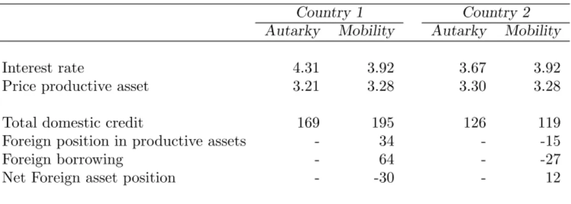
Interest rate 4.31 3.92 3.67 3.92

Price productive asset 3.21 3.28 3.30 3.28

Total domestic credit 169 195 126 119

Foreign position in productive assets - 34 - -15

Foreign borrowing - 64 - -27

Net Foreign asset position - -30 - 12

Note: Financial variables are in percentage of domestic output.

Before looking at the various asset positions with and without financial

integration, let’s look at the equilibrium interest rates. In both countries and

in both financial regimes, the interest rates are smaller than the

intertempo-ral discount rate 1

/β

−

1 ≈

0 .

06. This is the consequence of precautionary

savings from savers who face uninsurable idiosyncratic risks. Because

pro-ducers do not face any uncertainty (absence of precautionary motives), the

low interest rate implies that they will borrow as much as possible. Therefore,

the borrowing limit (7) is binding.

We can now look at the stock positions of the two countries. In the steady

state without capital mobility (autarky), the domestic credit of country 1 is

169 percent the value of domestic output while in the steady state with

financial integration this is 195 percent.

10

_{Therefore, the model predicts}

that capital markets liberalization has contributed to an increase in domestic

credit of 26 percentage points the value of domestic output. In country 2,

instead, capital liberalization has generated a decline in domestic credit of 7

percentage points.

10_{Domestic credit is the sum of loans taken by producers plus the net worth of savers if}

this is negative. Because the value of the contingent claims can be negative, some savers are actually borrowing. However, the debt of savers is small in aggregate.

(22)

Capital liberalization has also induced country 1 to accumulate a

posi-tive net position in the producposi-tive asset of 34 percent the value of domestic

output.This is associated to an increase in foreign borrowing of 64 percent.

11

Therefore, after capital markets liberalization, the net foreign asset position

of country 1 reaches the long-term value of minus 30 percent.

The mechanism leading to these changes can be explained as follows.

As can be seen from Table 1, in the pre-liberalization equilibrium country

1 has a higher interest rate and a lower price of the productive asset than

country 2. Prices equalize after liberalization. Therefore, in country 1 the

interest rate declines and the price of the productive asset increases. This

allows producers in country 1 to increase borrowing since the higher price

of the productive asset increases the value of the collateral. At the same

time, because producers in country 1 face enforcement constraints that are

less tight than in country 2, that is,

ψ

1

_{> ψ}

2

_{, we can see from condition (10)}

that they require a lower return on the productive asset compared with the

return required by producers in country 2. The concavity of the production

function then implies that producers in country 1 operate larger scales. This

contributes to the positive position of country 1 in the productive asset.

To understand the negative net foreign asset position, we have to consider

the role played by savers. Because the interest rate in country 1 declines while

in country 2 increases (compared to the autarky equilibrium), savers decrease

their savings in country 1 and save more in country 2. As a result, a large

fraction of borrowing from producers is financed by foreign savers through

the banking system.

To summarize, the model captures the fact that capital liberalization

has contributed to generating a significant amount of foreign borrowing for

country 1, the US. The increase in borrowing induced by capital markets

liberalization is in the order of 64 percent the value of domestic income.

11_{The net foreign position in the productive asset is the difference between the total}

productive assets owned by domestic producers and the domestic endowment of the asset, ¯

k, multiplied by the market pricePi

t. Foreign borrowing is the difference between domestic

credit, defined in the previous footnote, and the total loans made by domestic banks, that is, loans financed by the ‘positive’ claims of domestic savers and the equities of domestic banks.

(23)

3.2 Shock to bank equity and the short-term effects of capital

liberalization

In this section we address the second and third questions asked in the

In-troduction: Did the higher US leverages induced by globalization make the

current crisis worse? Did globalization allow the crisis to spread to other

countries?

In order to address these two questions we have to specify the driving

force behind the recent crisis. Although the events leading to the crisis are

complex and connecting the causes of these events to only one factor provides

an incomplete picture, there is no doubt that the balance sheet deterioration

of financial intermediaries played an important role. Therefore, we consider

a shock that decreases the equities of banks by a certain percentage of

out-standing loans. This can be interpreted as unexpected losses due to

unre-coverable loans made to producers. The goal of the paper is to understand

the consequences of these losses.

We consider a shock that generates a loss of bank equity in country 1

of 0.5 percent the value of worldwide loans. This is equivalent to about

1.5 percent the value of loans made in country 1. We start by studying

the impulse responses of asset prices which are reported in Figure 3 for the

economies with and without international mobility of capital.

Consider first the regime with capital mobility. As shown by the

continu-ous line, the shock generates an initial drop in the price of assets of about 13

percent. In considering the transition dynamics, the cost of avoiding bank

capital requirement plays an important role. This is captured by the

param-eter

κ

, which in the simulation is set to 0.1. As banks become unable to fulfil

the whole demand of loans without violating the capital requirement, they

start charging the additional financial cost. Higher values of

κ

increase this

cost more rapidly and induce a larger drop in the demand for loans. This,

in turn, generates a larger drop in asset prices.

12

Figure 4 plots the impulse responses for other variables (in levels) but

only in the case with capital mobility. The interest rate drops as banks

demand less deposits from savers in response to the reduction in the demand

of loans. The demand of loans decreases because of the higher marginal cost

of loans for producers, the ratio (1 +

r

i_t

)

/

(1

−

ϕ

i_t,l

(

l

t+1

)). The total volume of

loans made by banks contracts significantly and, as a result, producers cut

12_{As we increase}_κ_{, the response of asset prices becomes larger. However, for very large}

(24)

Figure 3: Impulse response of asset prices to an unanticipated shock to bank

equities. Economy with and without mobility of capital.

their consumption initially.

Next we consider the asset price response to the same shock but in the

regime without mobility of capital. As before, the shock derives from losses

made on country 1 loans. In the environment with mobility of capital it

does not matter whether the losses come from loans made in country 1 or

country 2. With capital mobility, in fact, firms can borrow indistinguishably

from domestic and foreign banks. Therefore, what matters is the worldwide

lending capacity of the whole banking sector. In the regime without capital

mobility, however, whether the losses are in country 1 or 2 matters. Only the

country in which the losses are materialized faces the type of consequences

shown in Figure 3 by the dashed line. Comparing the economies with and

without mobility of capital, we observe that the response of asset prices is

much bigger in the autarky regime.

Why is the asset price drop bigger in the autarky regime? The key to

the answer is the fact that globalization creates larger financial markets.

While in a closed economy borrowing is limited to the funds supplied by

(25)

Figure 4: Impulse response of asset prices to an unanticipated shock to bank

equities. Economy with mobility of capital.

(26)

domestic intermediaries, in a globalized economy producers can also borrow

from foreign intermediaries. As a result, in a globalized world the credit

contraction and the impact on aggregate prices are spread among all countries

that are financially integrated. The effect on country 1 is then smaller.

This finding seems to provide a negative answer to the question of whether

globalization made the crisis worse for the United States. More specifically,

the simulation exercise suggests that the crisis could have been much worse if

the US economy was not financially integrated in the world financial market.

However, this is an incomplete thought because it misses the fact (which is

consistent with the model) that leverage in the U.S. economy rose sharply

because of financial integration. Without financial integration, the economy

would have been less leveraged (as shown in the previous section), and hence

the aggregate volume of loans would have been smaller. Consequently, it

would have been possible that the losses incurred by financial institutions

and/or their likelihood were smaller. If we assume that the losses for the

banking sector are proportional to the stock of loans, then it is true that

the initial losses for banks in country 1 are smaller given the lower leverage.

However, the response of asset prices would still be higher than in the regime

with capital mobility. We will come back to this point in Section 5.

The results shown in Figures 3 and 4 also provide an answer to the

ques-tion of whether globalizaques-tion allowed the crisis to spill over other countries.

Here the model provides a clear answer: Although the impact on the

originat-ing country is smaller (as discussed above), other countries will be affected

by the shock even if the shock originated abroad. Therefore, with globalized

markets, country-specific shocks propagate to other economies inducing a

worldwide drop in asset prices.

4 Mark-to-market accounting

In this Section we explore how changes in the accounting principle used to

value assets in the banks’ balance sheet modifies the response of the model

to the initial financial shock. In the previous simulations we assumed that

the ‘equity’ of financial intermediaries relevant for the capital requirement

was determined by valuing assets at market prices. More specifically, capital

was valued at price

P

t

. Therefore, we assumed a mark-to-market approach.

We now consider an alternative scenario in which the banks’ assets are

valued at historical prices for the purpose of capital requirement, that is, for

the application of the constraint ¯

L

t+1

≤

α

(

e

t

−

d

t

). In our context this means

(27)

that in order to calculate the value of bank equities, the asset ¯

k

f

_continues

to be valued at the steady state price ¯

P

even if the market price changes.

Using (12), the capital requirement can also be expressed as:

¯

L

t+1

≤

α

k

¯

f

P

¯

+

L

t+1

1 +

r

i t

−

B

t+1

1 +

r

i t !