VYSOKÉ UČENÍ TECHNICKÉ V BRNĚ
BRNO UNIVERSITY OF TECHNOLOGYFAKULTA INFORMAČNÍCH TECHNOLOGIÍ
ÚSTAV INFORMAČNÍCH SYSTÉMŮ
FACULTY OF INFORMATION TECHNOLOGY DEPARTMENT OF INFORMATION SYSTEMS
IN-MEMORY DATABASES
DATABÁZY PRACUJÚCE V PAMÄTIBAKALÁŘSKÁ PRÁCE
BACHELOR‘S THESISAUTOR PRÁCE
JAKUB MOŽUCHA
AUTHOR
VEDOUCÍ PRÁCE
Doc. Ing. JAROSLAV ZENDULKA, CSc.
SUPERVISOR
Abstrakt
Táto práca sa zaoberá databázami pracujúcimi v pamäti a tiež konceptmi, ktoré boli vyvinuté na vytvorenie takýchto systémov, pretože dáta sú v týchto databázach uložené v hlavnej pamäti, ktorá je schopná spracovať data niekoľkokrát rýchlejšie, ale je to súčasne nestabilné pamäťové medium.
Na podloženie týchto konceptov je v práci zhrnutý vývoj databázových systémov od počiatku ich vývoja až do súčasnosti. Prvými databázovými typmi boli hierarchické a sieťové databázy, ktoré boli už v 70. rokoch 20. storočia nahradené prvými relačnými databázami ktorých vývoj trvá až do dnes a v súčastnosti sú zastúpené hlavne OLTP a OLAP systémami. Ďalej sú spomenuté objektové, objektovo-relačné a NoSQL databázy a spomenuté je tiež rozširovanie Big Dát a možnosti ich spracovania.
Pre porozumenie uloženia dát v hlavnej pamäti je predstavená pamäťová hierarchia od registrov procesoru, cez cache a hlavnú pamäť až po pevné disky spolu s informáciami o latencii a stabilite týchto pamäťových médií.
Ďalej sú spomenuté možnosti usporiadania dát v pamäti a je vysvetlené riadkové a stĺpcové usporiadanie dát spolu s možnosťami ich využitia pre čo najvyšší výkon pri spracovaní dát. V tejto sekcii sú spomenuté aj kompresné techniky, ktoré slúžia na čo najúspornejšie využitie priestoru hlavnej pamäti.
V nasledujúcej sekcii sú uvedené postupy, ktoré zabezpečujú, že zmeny v týchto databázach sú persistentné aj napriek tomu, že databáza beží na nestabilnom pamäťovom médiu. Popri tradičných technikách zabezpečujúcich trvanlivosť zmien je predstavený koncept diferenciálnej vyrovnávacej pamäte do ktorej sa ukladajú všetky zmeny v a taktiež je popísaný proces spájania dát z tejto vyrovnávacej pamäti a dát z hlavného úložiska.
V ďalšej sekcii práce je prehľad existujúcich databáz, ktoré pracujú v pamäti ako SAP HANA, Times Ten od Oracle ale aj hybridných systémov, ktoré pracujú primárne na disku, ale sú schopné pracovať aj v pamäti. Jedným z takýchto systémov je SQLite. Táto sekcia porovnáva jednotlivé systémy, hodnotí nakoľko využívajú koncepty predstavené v predchádzajúcich kapitolách, a na jej konci je tabuľka kde sú prehľadne zobrazené informácie o týchto systémoch.
Ďalšie časti práce sa týkajú už samotného testovania výkonnosti týchto databáz. Zo začiatku sú popísané testovacie dáta pochádzajúce z DBLP databázy a spôsob ich získania a transformácie do použiteľnej formy pre testovanie. Ďalej je popísaná metodika testovania, ktorá sa deli na dve časti. Prvá časť porovnáva výkon databázy pracujúcej v disku s databázou pracujúcou v pamäti. Pre tento účel bola využitá databáza SQLite a možnosť spustenia databázy v pamäti. Druhá časť testovania sa zaoberá porovnaním výkonu riadkového a stĺpcového usporiadania dát v databáze pracujúcej v pamäti. Na tento účel bola využitá databáza SAP HANA, ktorá umožňuje ukladať dáta v oboch usporiadaniach. Výsledkom práce je analýza výsledkov, ktoré boli získané pomocou týchto testov.
Abstract
This bachelor thesis deals with in-memory databases and concepts that were developed to create such systems. To lay the base ground for in-memory concepts, the thesis summarizes the development of the most used database systems. The data layouts like the column and the row layout are introduced together with the compression and storage techniques used to maintain persistence of the in-memory databases. The other parts contain the overview of the existing in-memory database systems and describe the benchmarks used to test the performance of the in-memory databases. At the end, the thesis analyses the results of benchmarks.
Klíčová slova
Databáza pracujúca v pamäti, databáza, IMDB, pamäťová hierarchia, usporiadanie dát, skladovacie techniky, testovanie výkonu, SQLite, SAP HANA, Python.
Keywords
In-memory database, database, IMDB, memory hierarchy, data layout, storage techniques, benchmarks, SQLite, SAP HANA, Python Language.
Citation
In-Memory Databases
Declaration
I declare, that this thesis is my own work that has been created under the supervision of Doc. Ing. Jaroslav Zendulka, CSc. All sources and literature that I have used during elaboration of the thesis are correctly cited with complete reference to the corresponding sources.
……… Jakub Možucha May 19, 2014
Acknowledgements
I would like to thank Doc. Ing. Jaroslav Zendulka, CSc., for his lead and valuable suggestions.
© Jakub Možucha, 2014.
Tato práce vznikla jako školní dílo na Vysokém učení technickém v Brně, Fakultě informačních technologií. Práce je chráněna autorským zákonem a její užití bez udělení oprávnění autorem je nezákonné, s výjimkou zákonem definovaných případů..
Contents
Contents ... 1
1 Introductions ... 3
2 Disc-Based Databases ... 4
2.1 Stone Age of Databases ... 4
2.2 Relational Databases ... 5
2.2.1 Relational Data Model ... 6
2.2.2 SQL Language ... 6
2.2.3 OLTP Systems ... 7
2.2.4 OLAP Systems and Cube Techniques ... 7
2.3 Object and Object-Relational Databases ... 8
2.4 NoSQL Databases ... 8
2.5 Big Data ... 9
3 Data in In-Memory Databases ... 10
3.1 Memory Media ... 10
3.1.1 Memory Media Types ... 10
3.1.2 Performance, Price and Latency of Memory Media ... 11
3.2 Data Layout in Main Memory ... 12
3.2.1 Row-Based Data Layout ... 12
3.2.2 Column-Based Data Layout ... 13
3.2.3 Compression Techniques ... 14
4 Storage Techniques in In-Memory Databases ... 15
4.1 Insert-Only ... 15
4.1.1 Point Representation ... 15
4.1.2 Interval Representation ... 16
4.2 Differential Buffer ... 16
4.2.1 The Implementation of Differential Buffer... 17
4.2.2 Validity Vector ... 17
4.3 The Merge Process ... 17
4.4 Logging and Recovery ... 18
4.5 On-the-Fly Database Reorganization ... 19
4.5.1 Reorganization in a Row Store ... 19
4.5.2 Reorganization in a Column Store ... 19
5 Existing In-Memory Databases ... 20
5.1 Observed Properties ... 20 5.2 SAP HANA ... 20 5.3 Times Ten ... 20 5.4 Kognitio ... 21 5.5 SQLite ... 21 5.6 An Overview ... 21
6 Performance Testing ... 22
6.1 Test Data ... 22
6.2 Test Queries ... 24
6.2.1 Tests on a Single Table ... 24
6.2.2 Tests on Several Tables ... 25
6.3 Methodic of Testing ... 26
6.3.1 Common Methodic ... 26
6.3.2 SQLite-Part Methodic ... 26
6.3.3 SAP HANA-Part Methodic ... 26
6.4 Test results ... 27
6.4.1 SQLite-Part Results ... 27
6.4.2 SAP HANA-Part Results ... 31
7 Analysis of Results ... 36
7.1 The Comparison of the In-Memory and the Disk Database ... 36
7.2 The Comparison of the Column-Based and the Row-Based Data Layout ... 36
8 Conclusion ... 37
Bibliography ... 38
1
Introductions
The growth of data that is needed to be processed is rising every year. Database systems along with other file storage systems need to be constantly developed and new concepts have to be examined to fulfill current needs for data processing. One of such concepts are in-memory databases, working in the fast main memory. The main goal of this thesis is to introduce the in-memory databases, explain the main features of these systems such as data layout for fast data access, compression techniques and storage techniques, which make the in-memory databases the mature systems ready to be used for enterprise needs. Output of this thesis will be series of tests, which will compare the performance of the in-memory database to the disk database and the performance of the in-memory database using the row-based data layout to the column-based data layout.
The thesis is divided into eight chapters. Chapter 2 will introduce the database systems and briefly summarize the mostly used concepts and systems for better understanding of database technology. Chapter 3 studies the data storages and layouts of stored data in main memory. Chapter 4 studies the techniques used to maintain data persistence in the in-memory database, since all the data in the in-memory databases are stored in the volatile media. Chapter 5 provides the overview of some existing in-memory systems and compares the degree of implemented in-memory technologies, since the in-memory databases are rather recent systems with different maturity. The tests used to compare the database performance are listed in chapter 6 along with description of test data and methodic of testing. Chapter 7 provides analysis of the test results and chapter 8 discusses the achieved results and proposes the further usage of the in-memory systems.
2
Disc-Based Databases
Achievements in database research have played very important role in the history of software development beginning in the 1960s and 1970s. Database system products had major impact on the growth of software industry and provided an efficient way to build communication, transportation, logistics, financial, management and defense systems, which were characterized by four requirements (1):
1. Efficiency in the modification and access to large amounts of data
2. Resilience, the ability to keep data in consistent state after system or software errors
3. Access control, including simultaneous access to data by multiple users and assuring authorized access to the data
4. Persistence, the maintenance of data over long periods of time, independent of the programs accessing the data
Database management systems (DBMS) along with specialized user-oriented query languages are today part of every system environment and provide easy way to organize, create and maintain collections of information important for system development. The following sections will provide the short overview over the most important milestones and trends in DBMS development from 1970s until today.
2.1
Stone Age of Databases
Before 1970, there were two mainly used DBMS:
1. Hierarchical databases where all records were organized into the collections of trees. One of the first hierarchical DBMS was IMS (Information management system) brought by IBM. IMS came with low-level query language by which a programmer could navigate from one root record to another, accessing one record at time.
2. Network databases where all the data were organized as a directed graph. These systems were built on the CODASYL standard brought by Conference on Data Systems Languages. These databases came with another query language that was able to access one record after another.
These approaches caused, that for every database request, there had to be the whole complex program written and the program had to be rewritten with almost every structure change of the database. At the result these databases were very costly to use and maintain (2).
2.2
Relational Databases
Relational databases have replaced the hierarchical and the network databases and are the most widely used DBMS in various forms. The paper written by E.Codd 1970 called “A Relational Model of Data for Large Shared Data Banks” with fundamentally different approach introduced the relational data model. All data are represented by tabular data structures (relations) and are processed by a high-level declarative language, which identifies the desired records. After this publication was published, the intensive investigation of relational DBMS concept began. The result was the great amount of commercial products based on relational concept which appeared in 1980s. In 1985, fifteen years after his first work on relational model, E.F.Codd introduced 12 rules for relational database management systems (RDBMS), which are commonly known as “Codd’s rules” (3):
1. The Information Rule
All information in the relational database is represented only one way - by values in tables.
2. Guaranteed Access Rule
Each and every datum (atomic value) is guaranteed to be logically accessible by resorting to a combination of table name, primary key value, and column name.
3. Systematic Treatment of NULL Values
Null values (distinct from empty character string or a string of blank characters and distinct from zero or any other number) are supported in the fully relational DBMS for representing missing information in a systematic way, independent of data type.
4. Dynamic On-line Catalog Based on the Relational Model
The database description is represented at the logical level in the same way as ordinary data, so authorized users can apply the same relational language to its interrogation as they apply to regular data.
5. Comprehensive Data Sublanguage Rule
A relational system may support several languages and various modes of terminal use. However, there must be at least one language whose statements are expressible, per some well-defined syntax, as character strings and whose ability to support all of the following is comprehensible: data definition, view definition, data manipulation (interactive and by program), integrity constraints, authorization, transaction boundaries (begin, commit, and rollback).
6. View Updating Rule
All views that are theoretically updateable are also updateable by the system
7. High-Level Insert, Update, and Delete
not only to the retrieval of data but also to the insertion, update, and deletion of data.
8. Physical Data Independence
Application programs and terminal activities remain logically unimpaired whenever any changes are made in either storage representation or access methods.
9. Logical Data Independence
Application programs and terminal activities remain logically unimpaired when information preserving changes of any kind that theoretically permit unimpairment are made to the base tables.
10. Integrity Independence
Integrity constraints specific to a particular relational database must be definable in the relational data sublanguage and storable in the catalog, not in the application programs.
11. Distribution Independence
The data manipulation sublanguage of a relational DBMS must enable application programs and terminal activities to remain logically unimpaired whether and whenever data are physically centralized or distributed.
12. Nonsubversion Rule
If a relational system has or supports a low-level (single-record-at-a-time) language, that low-level language cannot be used to subvert or bypass the integrity rules or constraints expressed in the higher-level (multiple-records-at-a-time) relational language.
These rules were a big step in determining, whether the used database system is really relational and provided guidelines and challenges for database system developers, because even until today, there is no RDBMS that would fully conform to these ideal rules.
2.2.1
Relational Data Model
Relational databases are based on relational data model. The data are organized by relations (tables) consisting of tuples (rows, records) with consistent attributes (4). Each record in table is uniquely indentified by a primary key, which is stored as an attribute or a combination of attributes. For example, a person can by identified in a table by his birth number or ID number. The relations between tables are expressed by foreign key, which is stored as an attribute. For example, the attribute ‘birth_town’ in table ‘Persons’ references the specific record from table ‘Towns’ by its value.
2.2.2
SQL Language
The RDBMS act on the data with operations of relational algebra like projections, selections, joins etc. It is highly formal mathematical language, unpractical for everyday use. Therefore RDBMS offer a layer above relational algebra, which is easier to understand and can be mapped to relational operations. Since 1970, there were such languages and the most popular was SEQUEL, later renamed
to SQL and first time standardized in 1986 (5). Nowadays is SQL the most used language for relational database operations with the current standard SQL 20111. SQL can be divided into four parts. The first part is DDL – Data Definition Language used to define data structures using operations like CREATE, ALTER, DROP or TRUNCATE. The second part is DML – Data Manipulation Language used to run operations on data such as INSERT, DELETE, UPDATE and most often used operation – SELECT. The third part is VDL – View Definition Language used to define user views and their mapping to the conceptual schema. The last and the most rarely used part is SDL – Storage Definition Language used to define storage options and local specialties of selected DBMS.
2.2.3
OLTP Systems
The most widespread RDBMS technology classes are OLTP and OLAP systems. Online Transaction Processing (OLTP) systems are able to provide a high number of concurrent online transactions, work with simple queries and are mainly used to store data (6). As part of OLTP systems research was developed the transactional concept which represents the transaction as a sequence of operations that must meet ACID guarantees (7):
1. Atomicity: guarantees that either all the updates of transaction are commited or no updates are commited/executed.
2. Consistency: guarantees that all the data will be consistent and none of the constraints on related data will be violated by transaction
3. Isolation: guarantees that the updates of a transaction cannot be seen by other concurrent transactions until the transaction is commited/executed.
4. Durability: guarantees that the updates of a transaction cannot be lost after the transaction is commited
Another concept used in OLTP systems is database distribution (2) developed in 1980s. This concept expects that data are not integrated in one system but decentralized to the more sites often to the heterogeneous OLTP systems. This approach moves data closer to the end user and also improves the availability of the database during system crashes.
2.2.4
OLAP Systems and Cube Techniques
The need to process and analyze very large amounts of data led to the conclusion, that the OLTP systems are not suitable for large data analytics because of their high complexity and long calculation time (6). The result was the rise of the OLAP (Online Analytical Processing) systems in 1990s. The OLAP systems are not suitable for transactions, data are regularly, but not often changed (once a week, or once a longer time), are separated from OLTP system's data and are used to analyze historical data using complex queries.
Cube techniques are used to analyze data stored in relational databases in different scenarios, from a variety of perspectives to support decision making. Cubes are organized, usually pre-processed, aggregated data structures. They can be created from multiple sources and are defined by dimensions and measures. Because of pre-processing, cubes provide mechanism for quick querying of multidimensional data. The term “cube” does not mean, that these data structures are limited to be only 3D. They can be really multidimensional, for example, the MS Server 2000 allowed 64 dimensions (8). Cubes are created from the set of joined tables called schema. There are two common types of schema – star schema and snowflake schema. Star schema consists of dimension tables joined to one fact table. Snowflake schema is an extension to star schema and same as star schema consists of one fact table and multiple dimension tables. The difference is that dimension tables can join another dimension table. There are also other types of schema, for example galaxy, which consists of two or more fact tables joined to dimensions. Every dimension can include a hierarchy to provide different levels of information. For example the “Date” dimension includes level hierarchy: decade, year, month, week and day. User can query the information for the higher level and then expand the dimension hierarchy to see more details. Cubes are the technology mostly used within Relational and Multidimensional Online Analytical Processing (ROLAP & MOLAP). These systems enable interactive analyses of multidimensional structured data. The drawback of using ROLAP or MOLAP is the need to pre-process the cubes, which requires even more storage capacity and increases data redundancy.
2.3
Object and Object-Relational Databases
In 1990s, the object oriented languages have spread heavily. This caused the need to develop the DBMS to store the objects, their inheritance, hierarchies and ensure their lasting persistence. The RDBMS are eligible to store simple data and an enormous effort has to be taken to decompose the object data to relation data and results in high complexity of source code and magnificent computing power loss. This need resulted in relational-object databases and object databases.
The object-relational databases are the extensions of relational databases with data model adapted to support inheritance and methods with the extended query language to support these types of operations. These extensions were added to the SQL standard in 1999, allowing relational databases to support object concepts (9).
The object databases are based on brand new data model with object concepts such as encapsulation, methods, inheritance, polymorphism and identity of an object. These databases do not share any common query language (10).
2.4
NoSQL Databases
In late 1990s, the first NoSQL databases appeared. NoSQL stands for not only SQL, which means that other data models than relational are available, which is in opposition to the traditional relational systems. The main difference is the ability to store records with different attributes in one table. These
systems are more simple to use and faster than traditional relation systems and are also popular for their usage in cloud. There are many models of NoSQL databases such as Key-value databases,
Document databases, Graph databases, Object databases, etc. The main disadvantage of NoSQL systems is the unability to provide ACID guarantees and the fact, that there is no shared common query language except of the few ones, which support also the SQL (11).
2.5
Big Data
Nowadays, the term ‘Big Data’ is used still more and more. Due to social sites, digitalization and worldwide information overwhelm it is a new challenge for companies, to be able to process data so huge, that the size itself becomes a part of research problem. Just for example, the IBM statistics show, that daily amount of generated data in 2012 was nearly 2.5 exabytes and this amount is growing 60% annually2. The main characteristics of Big Data are:
1. Volume – each day Google has to process 20PB, Facebook and Twitter together generate more than 17TB of data
2. Velocity – most of the data have to be processed and accesible in real-time (GPS data)
3. Variety – data are stored in unstructured format – text, audio, video (100 hours of video is uploaded on Youtube every minute3)
For processing such data were developed many strategies. First and most widespread is to improve hardware performance and capacity. This contains development of faster machines, using multi-core technologies, new and cheaper storage and faster throughput. Second widely used strategy is the support of maximum parallel processing (12).
Almost the synonym for processing of big unstructured data is Hadoop. Companies like Facebook, Yahoo!, Twitter use this system to store and process their data. Hadoop is based on MapReduce framework created by Google in 2004 and its main purpose was to store and process a huge amount of unstructured data. However, the latest versions of Hadoop are also improving in processing of structured data, this system is not really a database system, rather the file system. Data are multiple stored in HDFS (Hadoop File Systems), which create clusters and even collections of clusters to enable the most important characteristic of Hadoop – massive parallelism. To access data, first step, the map function maps all the data by chosen key through the data clusters. The second step is the
reduce function to reduce all duplicate values found by map function (13).
The last versions of Hadoop provide also support for analysis of structured data (SQL queries). However the best results give in processing of unstructured data and therefore is very often used as preprocessor, which provides structured data databases.
2
http://www.marketingtechblog.com/ibm-big-data-marketing/#gsc.tab=0 3 http://www.youtube.com/yt/press/statistics.html
3
Data in In-Memory Databases
The in-memory databases (IMDB) are the answer to the latest requirements for the enterprise computing but also a result of many years of research, which builds on the results of previous DBMS and moves them from disc to main memory. One of the greatest requirements was the need for real-time processing of Big Data. The second requirement was to create the single source of data for modern enterprise applications instead of having OLTP and OLAP – the two separated systems. Modern application has to process data from multiple sources and the division to two separated systems has the following drawbacks (14):
The OLAP systems do not have the latest data.
For better performance work the OLAP systems with predefined materialized aggregates (cubes), which limits the user query possibilities.
Data redundancy is high due to similar information stored in both systems.
The schemas for the OLTP and OLAP systems are different, which creates complexity to use them and to synchronize data between them.
One of the first studies on in-memory databases was published in 1992 by H.Garcia-Molina and K.Salem in their paper „Main memory database systems: An Overview“, where they introduced in-memory concept along with issues that has to be solved to be able to construct such systems (15). Following sections will deal with fundamentals of in-memory technology and issues the researchers had to solve to create such systems.
3.1
Memory Media
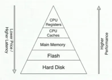
To better understand, how the data are stored and how it influences the speed of data processing in databases, it is important to take look at the memory hierarchy of computers. Computers consist of more than just one type of memory mediums which are ordered as the layers from the CPU to the last memory level – the hard drive.
Very important monitored measure in memory data access is latency. Latency is the time delay, that it takes the system to load the data from the storage medium to make it available for the CPU. This delay increases with the distance of data from the CPU.
3.1.1
Memory Media Types
The first level are the registers inside the CPU. These registers store the inputs and outputs of instructions processed by CPU. Every processor has a small amount of registers, which can store integer and floating point values, nowadays with size of 32 or 64 bits (depending on architecture) and can be accessed really fast. All the data processors work with has to be first loaded and stored in registers from other types of memory to be accessible for the CPU.
The second level of computer memory are the caches. Each CPU core has its own L1 and L2 cache and one bigger L3 cache, which are able to store from kilobytes to megabytes of data. Caches are built out of SRAM (Static Random Access Memory) cells which usually consist from 6 transistors. This technology is very fast but requires a lot of space. The data in caches are organized in cache lines, which are the smallest addressable units with size of 64 bytes. If the requested data cannot be found in cache, they are loaded from the main memory, which is another layer in memory hierarchy. The modern processors also try to guess, which data will be used next and load these data to reduce the access latency since the latency of L1 and L2 caches can be measured in nanoseconds, which is many times less than the latency of other memory media (16).
Main memory is the third level of memory hierarchy and is built out of DRAM (Dynamic Random Access Memory) cells. These cells are simpler and more economical than SRAM cells and consist from only one transistor used to guard the access to the capacitor, where is stored the state of memory cell. However, there is complication with capacitor discharging over the time. Therefore, the system has to refresh DRAM chips every 64 ms and after every read to recharge the capacitor. During the refresh, the state of cell is not accessible and causes the limited speed of DRAM chips. The latency of the main memory can be measured in hundreds of nanoseconds (17).
The CPU registers, caches and main memory are all volatile media. This means, that they can store information until they are plugged to the power source. When they are unplugged, the all data they have held disappear. The opposite are the non-volatile technologies like flash and hard disks, which are used as permanent storages for data.
3.1.2
Performance, Price and Latency of Memory Media
The memory hierarchy can be viewed as a pyramid on Fig. 3-1. The higher is the memory type in the pyramid, the better performance in data processing it achieves and the lower is the latency.
On the other hand, the lower is the memory media type in the pyramid, the cheaper it gets and therefore is suitable to store bigger amounts of data. In latest years, the price of main memory decreased rapidly and this trend made it possible to even think about databases stored fully in main memory because it is now more affordable.
3.2
Data Layout in Main Memory
Relational database tables have two-dimensional structure and the question is, how to store the data in one-dimensional main memory storage to achieve the best performance in both analytical and transaction queries. There are two ways of representing a table in memory called row and columnar layout. To illustrate these two approaches I will use a simple example in Table 3-1 with all values stored as strings directly in memory.
Id
Name
Country
1
Peter Parker
USA
2
John Smith
Ireland
3
Paul Heinz
Germany
Table 3-1 Example table
3.2.1
Row-Based Data Layout
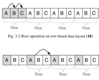
Row layout has been used in almost every disc-based relational database. To store data in row layout means, that the table is stored in memory row by row. Considering the example above, the data would be stored as follows: “1,Peter Parker,USA;2,John Smith,Ireland;3.Paul Heinz”
The data access on row-based data layout for row operation is illustrated on Fig. 3-2 and for column operation on Fig. 3-3.
Fig. 3-2 Row operation on row-based data layout (18)
It is clearly visible, that row layout offers effective data access for operations working with single row such as insert, delete or update – the transactional operations. This is the reason, why was using this layout in OLTP systems the best practice. On the other hand, it is not as effective for read operations which access only a limited set of columns since the data cannot be processed sequentially. The other disadvantage of read operations performed in row-based layout is the size of the data that is needed to be cached. For example, the “ID’ attribute from the table above can have the size of 11 bytes. However, when reading it, the smallest amount of data that can be cached is 64 bytes which results in 53 bytes of unused data cached for every row in table.
3.2.2
Column-Based Data Layout
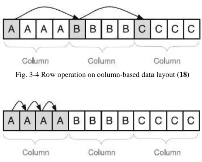
Column-based layout is concept where all data are stored attribute-wise, the values of one column are stored together column by column. Considering the example above, the data would be stored in following order: „1,2,3;Peter Parker,John Smith,Paul Heinz;USA,Ireland,Germany“.
The data access on column-based data layout for row operation is illustrated on Fig. 3-4 and for column operation on Fig. 3-5.
Fig. 3-4 Row operation on column-based data layout (18)
Fig. 3-5 Column operation on column-based layout (18)
It is clear, that the columnar layout is very effective for read operations where the values of one column can be read sequentially and no unnecessary data are cached. Another benefit of using columnar layout is the possibility to apply the efficient compression techniques described in following section. Third benefit is, that the sequentially read of values enables on the fly calculation of aggregates so storing of pre-calculated aggregates in the database can be avoided (14). This results in minimizing redundancy and complexity of database. Columnar approach on the other hand is not so efficient for transactional operations. However it can still achieve very good results caused by the
fact, that all data are stored in main memory and workloads of enterprise databases are more read-oriented.
3.2.3
Compression Techniques
In large companies, the size of data set can easily reach several terabytes. The prices of main memory are falling down, but it is still expensive to process huge sets of data fully in memory. Therefore there are multiple compress techniques (18) applicable mostly with columnar layout to decrease the memory requirements. Another impact is, that compression techniques also decrease the amount of data needed to be transferred between main memory and CPU registers, which increases the query performance.
Fig. 3-6 Dictionary encoding (18)
The first compression technique is called Dictionary encoding, which is also a basis for other compression techniques. This encoding works column-wise and is suitable for columns with high rate of same values. The concept of this encoding is very simple. Every distinct value in a column is replaced by a distinct integer value ID and the two or more records are created, one in dictionary table with value of column and value ID representing this value and a record or more records in attribute vector with value ID and all positions of the representing value in the table. The concept is illustrated on Fig. 3-6. Dictionary encoding is the only compression applicable also for row-based layout.
Another compression method is called Prefix Encoding which is the optimization of dictionary encoding. This encoding finds the most redundant value ID in attribute vector and creates the new prefix vector which contains the most redundant value ID, number of its occurrences and the rest if ID values with their positions.
Run-Length encoding is the compression which works only on column with few distinct value IDs. In Run-Length encoding the records in attribute vectors are replaced with records consisting of value ID and number of its occurrences or its starting offset in the column.
Delta encoding is the compression technique to reduce size of alpha-numerically sorted dictionary unlike the other ones used to compress the attribute vector. This encoding stores the common prefixes of the values in dictionary.
4
Storage Techniques in In-Memory
Databases
One of the transactions properties is durability. Durability means, that after the transaction is committed, any of the modifications cannot be lost. Technically it means, the changes have to be written on a durable, non-volatile medium (19). Since in-memory databases store all data in main memory, which is volatile, the researchers had to come with new storage techniques to ensure, that changes in in-memory databases are durable and database is able to recover after crashes.
4.1
Insert-Only
Data in enterprise databases change and these changes should be traceable to fulfill the law and financial analytics demands. There are many complicated technologies used to store historical data. Insert-only approach simplifies this task rapidly. Insert-only approach (18) means that tuples are not physically deleted or update but invalidated. Invalidation can be done by adding an additional attribute which indicates the tuple has been changed. This makes the accessing of historical data very simple, just by using the revision attribute value for the desired version. This approach also simplifies work with column dictionaries, since no dictionary cleaning is needed. There are two ways to differentiate between actual and outdated tuples.
4.1.1
Point Representation
To determine the validity of the tuple, the “valid from“ date attribute is stored with every tuple in database table, when using point representation. The field contains the date, when the tuple was created. Advantage of this method is the fast write of new tuples and the other tuples do not have to be changed. For example, to do the update on existing tuple, the user or application query looks like in Algorithm 4-1.
The update statement is automatically translated and Algorithm 4-2 statement is executed.
UPDATE world_poplation SET city = ‘Hamburg’
WHERE id = 1
Algorithm 4-1 Point representation user query
INSERT INTO world_population
VALUES (1, ‘Name‘ , ‘Surname‘ , ‘Hamburg’ , ‘Germany’ , ’10-5-2014’)
Disadvantage of this method is low efficiency of read operations. Each time when the search for a tuple is performed, the other tuples of that entry has to be checked to find the most recent one. All these tupples need to be fetched and sorted by “valid from” attribute. Point representation is efficient for OLTP operations, where the write operations are usually performed more than the read operations.
4.1.2
Interval Representation
When using interval representation, “valid from” and “valid to” attributes are stored with every tuple in the database table. These attributes represent the date of creation and invalidation of tuple. At updating of a record, the new tuple is stored with “valid from” attribute and “valid to” attribute changes in the old tuple. The interval representation is not as efficient for writes operation because two operations has to be done in this case (Algorithm 4-3 and Algorithm 4-4).
On the other hand, this method is suitable for read operations. There is no need to fetch and sort all the tuples of desired record but only the tuples with appropriate key and empty “valid to” date have to be selected. This is the reason, why this approach is more efficient for OLAP operations, where read operations are required more often than write operations.
4.2
Differential Buffer
In dictionary compressed table an insert of a single tuple can lead to restructuring of the whole table which also includes the reorganization of the dictionary and attribute vector. The solution to this problem is the concept, which divides the database into main store and differential buffer (18). Data in main store are stable and all modifications happen in differential buffer only while the state of data is calculated as the conjunction of the differential buffer and the main store. This means that every read operation has to be performed on the main store but also the differential buffer. However, the size of differential buffer is much smaller than the main store, this has only a small impact on read performance. The query is logically split into a query on the compressed main memory and the differential buffer and the final result has to be combined the results of both subsets.
UPDATE world_population
SET validTo = ’10-05-2014’
WHERE id = 1 and validTo is NULL
Algorithm 4-3 Interval representation user update query
INSERT INTO world_population
VALUES (1 , ‘Name’ , ‘Surname’ , ‘Hamburg’ ‘Germany’ , ’10-05-2014’ , NULL)
4.2.1
The Implementation of Differential Buffer
The concept of a column-based layout and the dictionary compressing is used also in differential buffer. Due to better write performance the dictionary is not sorted and the values are stored as inserted and to speed up the read accesses the values are organized in trees.
4.2.2
Validity Vector
To distinguish, which tuple in the main store and differential buffer is no longer valid, the system validity vector is added to the table. This validity vector stores a single bit for every tuple which indicates, if the tuple at this position is valid or not. In the query execution is query firstly executed without the validity vector interfering in the main store and in parallel in the differential buffer. After the result is compressed, the result positions are verified with the validity vector to remove all invalid results.
4.3
The Merge Process
The merge (20) is the cyclical process, when are the data from differential buffer combined with compressed main partition. Merging the data of the differential buffer into the compressed main store decreases the memory consumption due to better compression but also improves the performance due to the sorting of the dictionary of the main store. However, there are also requirements of the merge process:
1. Can by executed asynchronously
2. Has very little impact on all other operations 3. Does not block any OLTP and OLAP transactions
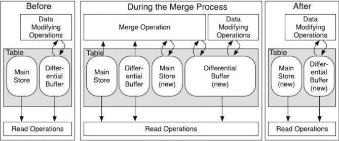
To achieve these requirements, the merge process creates a new empty differential buffer and the copy of actual main store to avoid interrupting during the merge. In this concept the old main store with old differential buffer and new differential buffer are available for reads and new data modifications are passed to the new differential buffer. Just to remind, all the updates and deletes are performed as technical inserts while validity vector ensures consistency. The read performance of differential buffer is decreased depending on the number of tuples in it especially the JOIN operations, which have to be materialized. The merge process has to be executed if the performance impact becomes too large and can be triggered by these events:
1. The number of tuples in differential buffer exceeds a defined threshold. 2. The memory consumption of the differential buffer exceeds a specified limit. 3. The differential buffer log exceeds the defined limit.
One of the requirements on the merge is that it should run asynchronously. This means that merge should not block any modifying operations. This is achieved by creating a new differential buffer during the merge process. Fig. 4-1 illustrates the concept of merge.
Fig. 4-1 The Merge Process (18)
The only locks that are required are at the beginning and the end of the process of switching the store and applying data modifications which have occurred during merge process. The changes of open transactions are copied from the old differential buffer to the new one and therefore are not affected be by the merge and can be run in parallel to the merge process. At the end of the merge process, the old main store is replaced with the new one. When all this is done, a snapshot of a database is taken and stored to the non-volatile medium. This step creates a new starting point for logging in case of failures. More on the logging is described in next sections.
4.4
Logging and Recovery
Logging is the standard procedure to enable durable recovery from the last consistent state before the failure. It means to check point the system and write all the modifications into the log files, which are stored on non-volatile media. This concept is applied in almost every database. However it had to be changed slightly for in-memory database requirements.
Check pointing is used to create a periodically snapshots (21) of the database to the persistence medium which are the direct copies of the main store. The purpose of periodically snapshots is to speed up the recovery since only log entries after the snapshot has to be replayed and the main store can be loaded directly to memory. After these processes are done, the database is back in consistent state.
4.5
On-the-Fly Database Reorganization
Database schema has to be changed time to time due to software changes or workload changes and the option for database reorganization such as adding an attribute to a table or changing attribute properties is required. The reorganization is very different comparing row-based and column-based layout in databases (18).
4.5.1
Reorganization in a Row Store
In row-based databases is the reorganization time-consuming and DBMS usually do not allow these changes while the database is online. This is caused by the fact, that data in row-based database are stored in the memory block sequentially row by row and each block contains multiple rows. If additional attribute is added or the size of attribute is changed, it requires the reorganization of the storage for the whole table.
To enable dynamically change of data layout, a logical schema has to be created on top of the physical data layout. This method decreases the performance because of the need to process data in logical tables which requires more computing than accessing the data directly.
4.5.2
Reorganization in a Column Store
In column-based layout, each column of the table is stored independently from the other columns in a separate block. New attribute is therefore added very easily, because it will be created in new memory area without the need to any reorganization.
5
Existing In-Memory Databases
This chapter will provide the description of the few chosen and most widespread in-memory database systems and the wider overview of existing in-memory database systems. The previous chapters provided an overview of characteristics of in-memory databases which are more or less adapted to the existing solutions.
5.1
Observed Properties
Writing about in-memory databases, the most important characteristic of a database is the data layout and the ratio of data in-memory to the data on the disk. There are databases that are fully in memory and the others which can be called hybrid databases allowing both ways of storing data. Some databases have also the main memory size limitations. Another important characteristic is the ability to provide parallel processing on single query since any conventional computer has more than one core nowadays.
Ability for vertical and horizontal scaling is another important characteristic. Vertical scaling (Scale-up) refers to adding more processors or main memory for the server. On the other hand, the horizontal scaling (Scale-out) refers to adding more servers, in other words building the clusters.
5.2
SAP HANA
SAP HANA (22) (High-Performance Analytic Appliance) is one of the most advanced in-memory databases available. Data in this database system are fully in-memory and the system provides both row-based and column-based data layout and also support for compression techniques based on columnar layout. Making most of the in-memory techniques, SAP HANA claims to be both OLAP and OLTP system. To run SAP HANA, it is recommended to have at least 64GBs of main memory, because only the system files that are also stored in memory have more than 12GBs, while there is theoretically no upper limit. However, there is no bigger main memory storage yet, than was built by IBM4 in 2012 and SAP HANA did run on 100TB main memory. Also, the support for scale-up and scale-out is provided and a query can be executed in parallel.
5.3
Times Ten
Times Ten database (23) is the OLTP in-memory system from Oracle. This system is fully in memory and can be used as standalone database but also as the cache system for other database system running on disk. However, this approach is not as efficient because of data redundancy. Main memory size is theoretically unlimited and there is also no minimal limit, practically there has to be enough memory to store and process data. Data layout is row-based and dictionary compression is
supported. Times Ten is able to scale-up, but scale-out is limited to 2TBs and parallelism of query is supported.
5.4
Kognitio
Kognitio (24) is the OLAP in-memory system working fully in memory. Data layout is row based and no compression techniques are recommended to use in this system. There is no main memory limit as well as no limit for scale-up and scale-out and supported parallel processing.
5.5
SQLite
SQLite is not primarily the in-memory database. However the temporary database can be created in memory mode having no durability guarantee in case of failures or even when the database is stopped without saving. SQLite is a lightweight database system which stores the whole database in the single database file. Data layout is row-based and the memory database is limited to 1TB. SQLite is independent from system scale-up, but there is no support for cluster creation since all data are stored in a single database file (25).
5.6
An Overview
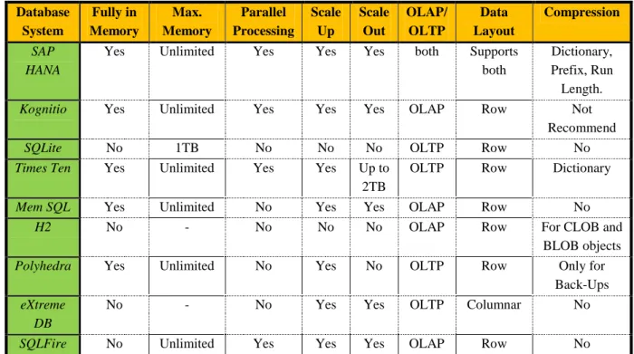
The following Table 5-1 provides the overview of the chosen and some extra in-memory systems and their characteristics. Database System Fully in Memory Max. Memory Parallel Processing Scale Up Scale Out OLAP/ OLTP Data Layout Compression SAP HANA
Yes Unlimited Yes Yes Yes both Supports
both
Dictionary, Prefix, Run Length.
Kognitio Yes Unlimited Yes Yes Yes OLAP Row Not Recommend
SQLite No 1TB No No No OLTP Row No
Times Ten Yes Unlimited Yes Yes Up to 2TB
OLTP Row Dictionary
Mem SQL Yes Unlimited No Yes Yes OLAP Row No
H2 No - No No No OLAP Row For CLOB and
BLOB objects
Polyhedra Yes Unlimited No Yes No OLTP Row Only for Back-Ups
eXtreme DB
No - No Yes Yes OLTP Columnar No
SQLFire No Unlimited Yes Yes Yes OLAP Row No Table 5-1 In-Memory Databases Overview
6
Performance Testing
Performance testing is divided into two parts. The first part of the testing is focused to compare the performance of database stored on disk to the performance of the database stored in main memory. For these tests is used SQLite database with its in-memory mode. The second part deals with performance of row-based layout data compared to the performance of the column-based layout and for these tests was used SAP HANA database running in a cloud as a Cloudshare5 service. The performance was tested by the set of ad-hoc queries.
6.1
Test Data
The first task was to retrieve the data for testing. The data come from The DBLP – Computer Science Bibliography Database, where are stored more than two millions of science bibliography records. However, this database is stored as a XML file, so the couple of steps had to be done to build test database.
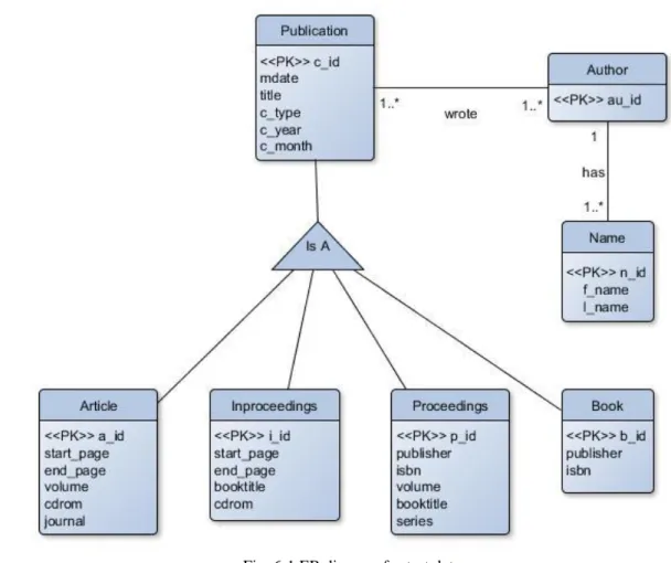
Fig. 6-1 ER diagram for test data
The first step was to create an ER diagram (Fig. 6-1) for the desired test database. The DBLP XML file contains the publication records of the following types: ‘article’, ‘proceedings’, ‘inproceedings’, ‘book’, ‘www’, ‘phdthesis’ and ‘mastersthesis’. The ‘phdthesis’ and ‘mastersthesis’ records are not included to the final test database, because of their very low frequency. The ‘www’ records can be also a home page records for the publication authors and all of their name synonyms are included in this record. To create the most possible complex system for the testing purposes, the central entity ‘Publication’ is created. This entity has the attributes that are common for all the publication types. For further attributes of publications, the other entities were created.
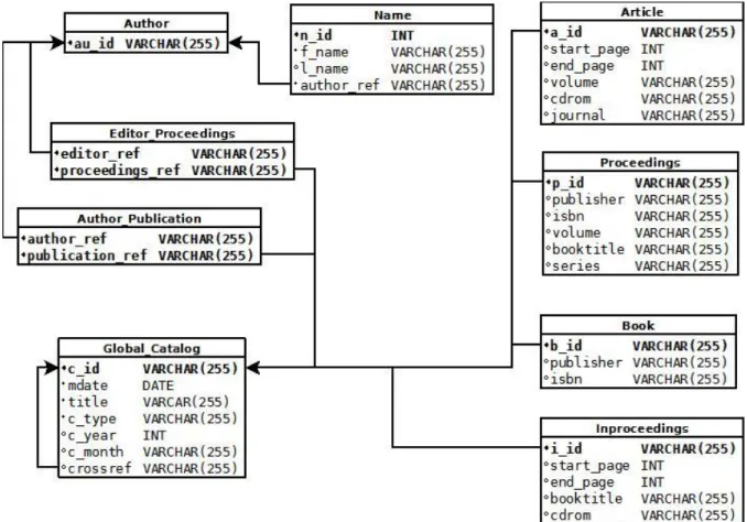
The second step was to create database schema that is illustrated in the Fig. 6-2. The ‘Publication’
entity was mapped to ‘Global_Catalog’ table for better understanding of the schema. The ‘crossref’ attribute are the values from ‘inproceedings’, which reference the ‘proceedings’ where they were published.
Fig. 6-2 Test Database Schema
The last step was to create the SQL file containing table definitions and CSV files containing data for tables for better import performance. To do this, I had to write a parser in Python 3, which parses the XML file and creates the CSV files with the data using the XML SAX parser library6. The source
code of this parser can be found in the appendix. However, the parser was not enough to create all the data. In the XML file, all the publication authors were written not as the author IDs, but as the names. This caused the complicated creation of ‘Author_Publication’ and ‘Editor_Proceedings’ tables, where all the records have to be in form of author and publication IDs. This issue was solved by loading all the data with publications, names and authors and combining them in SQLite database. In the result I got the database with size of 1.3GBs and more than 14 million rows together.
6.2
Test Queries
This section provides the overview of the ad-hoc queries used to test the read database performance. These tests are inspired by business question queries by TPC DS (26) benchmarks. The queries are divided into two main groups. In the first group are the queries working on one table and are divided into several groups according to their complexity. In the second groups are the queries working on several tables using joins or unions. Again, this group divided into two subgroups according to their complexity. In total, 23tests have been designed. The following section will provide the overview of the test on one table and their SQL representation. The tests on more tables that are listed in the next section have quite long and complex SQL code which can be found in the appendix. The results of the test are referred to as SQLite Test 1, SQLite Test 23 and SAP HANA Test 1, SAP HANA Test 21.
6.2.1
Tests on a Single Table
In this section are listed relatively simple ad-hoc queries working with one table with their SQL code. A. Queries with functions
1. Count how many publications are in database
SELECT count(*) FROM Global_Catalog
2. Compute the average year of creation of all publications
SELECT avg(c_year) FROM Global_Catalog
B. Queries with where clause
3. Count all titles of publications which have in their title 'database'
SELECT count(*) FROM Global_Catalog
WHERE title like '%database%'
4. Write titles of publications written in the latest year
SELECT title,c_year FROM Global_Catalog
WHERE c_year=(SELECT max(c_year) FROM global_catalog)
C. Queries with order clause 5. Order publication by year
6. Order publications by year and then date of database import
SELECT title FROM global_catalog ORDER BY c_year,mdate
7. Order names by last name
SELECT concat(f_name,concat(“ ”,l_name)) FROM Name
ORDER BY l_name
8. Write all ordered first names
SELECT distinct f_name FROM name ORDER BY f_name
D. Queries with aggregation
9. Write how many publication was written by years
SELECT c_year,count(*) FROM global_catalog GROUP BY c_year
10. Write how many publication was written by months and years
SELECT c_year,c_month,count(*) FROM global_catalog
GROUP BY c_year,c_month
11. Write which first names are the most used
SELECT f_name,count(*) FROM name
GROUP BY f_name
ORDER BY count(f_name) DESC
6.2.2
Tests on Several Tables
These are more complex queries using joins and unions on more tables. The SQL queries are rather complex and can be found in the appendix.
E. Queries with simple joins and unions
12. Write titles of proceedings and their inproceedings 13. Count all rows in database
14. Count all books and proceedings from publisher 'Springer' in specified 2005 F. Queries using joins and unions with order or aggregation clauses
15. Order author IDs by number of their synonyms 16. Order publications by length
17. Order authors by number of publication they wrote and edited 18. Order publishers by the amount of published publications
19. Find authors who wrote more than 2, but less than 5 publications 20. Find author, who have written the most articles in year 2005 21. Find authors, who wrote more inproceedings than articles 22. Count authors who have wrote only in year 2006.
23. Report all authors, number of his creations, number of editored proceedings,year when he wrote most, number of his synonyms
6.3
Methodic of Testing
In previous sections were presented the queries used for database performance testing in both test parts. Following subsections will show the methodic of testing and the steps that I had to take to run the tests and in the next section are the results of the tests.
6.3.1
Common Methodic
For performance testing, I have chosen to compare the time of execution, since it can be measured very simply. To get the most objective results from tests, I executed the whole set of queries ten times. I have chosen this approach instead of running one by one every test query ten times to overcome the use of cached data from previous execution of the query in repeated executions. After the results were given, the maximum and minimum times were removed and the average time of execution was computed from the rest of results.
6.3.2
SQLite-Part Methodic
To test the SQLite database in disk and memory mode I wrote a script in Python 3 using the SQLite3 library. At first, the script executes the queries on disk, stores the measured time of execution, computes the average time and creates a benchmark log file with the results. Afterwards, it closes the disk database, opens the in-memory database, loads data in the in-memory database, repeats the tests and writes the measured values to the log file. The illustration of the work with in-memory database in SQLite in Python 3 is in Algorithm 6-1. The whole script can be found in the attachments.
6.3.3
SAP HANA-Part Methodic
To compare the performance of the row-based and column-based data layout I used the almost same script as the one for SQLite-part testing. To connect to SAP HANA I used the dbapi library. At first,
import
sqlite3, time
memcon = sqlite3.
connect
(“
:memory:
”)
tempfile =
open
('backup.sql')
memcon.
cursor
().
executescript
(tempfile.
read
())
run_tests
(memcon,test_array,log)
memcon.
close
()
the script was executed on column-based tables. Then I changed the type of tables from column-based to row-based dynamically, which is very useful functionality in SAP HANA, and executed the tests again. The illustration of the work with dbapi library in Python 3 is in Algorithm 6-2. The whole script can be found in the attachments.
6.4
Test results
6.4.1
SQLite-Part Results
This section will provide the overview of the first-part test results on SQLite on the graphs referenced from SQLite Test 1 to SQLite Test 23 . The tests were run on the computer with the configuration listed in the Table 6-1.
Processor
Intel Pentium P6100 @2GHz Dual-Core
Main Memory
4GB DDR3 (1066 Mhz)
Operation System
Windows 7 Home Premium 64b
Python 3
3.2.5
SQLite 3
3.8.4.3
Table 6-1 SQLite test computer configuration
SQLite Test 1 [s] SQLite Test 2 [s]
Disk Memory 0 0,05 0,1 0,15 0,2 0,25 0,3 0,35 0,4 0,45 Disk Memory 0 0,2 0,4 0,6 0,8 1 1,2 1,4 1,6 1,8
import
dbapi
conn = dbapi.
connect
('
hanacloud
',30015,'
SYSTEM
','
manager
')
cur = conn.
cursor
()
start_time = time.
clock
()
cur.
execute
(test[
i
])
end_time = time.
clock
()
result_time = end_time - start_time
SQLite Test 3 [s] SQLite Test 4 [s]
SQLite Test 5 [s] SQLite Test 6 [s]
SQLite Test 7 [s] SQLite Test 8 [s]
Disk Memory 0 0,5 1 1,5 2 2,5 3 3,5 Disk Memory 0 0,5 1 1,5 2 Disk Memory 10,5 10,55 10,6 10,65 10,7 10,75 10,8 Disk Memory 12,75 12,8 12,85 12,9 12,95 13 13,05 13,1 13,15 13,2 Disk Memory 5,65 5,7 5,75 5,8 5,85 5,9 5,95 6 6,05 6,1 Disk Memory 3,2 3,4 3,6 3,8 4 4,2 4,4
SQLite Test 9 [s] SQLite Test 10 [s]
SQLite Test 11 [s] SQLite Test 12 [s]
SQLite Test 13 [s] SQLite Test 14 [s]
Disk Memory 5,4 5,5 5,6 5,7 5,8 5,9 6 6,1 6,2 Disk Memory 6,3 6,4 6,5 6,6 6,7 6,8 6,9 7 7,1 Disk Memory 4,8 5 5,2 5,4 5,6 5,8 6 6,2 Disk Memory 0 0,5 1 1,5 2 2,5 Disk Memory 0 5 10 15 20 25 30 35 40 Disk Memory 0 0,02 0,04 0,06 0,08 0,1 0,12 0,14
SQLite Test 15 [s] SQLite Test 16 [s]
SQLite Test 17 [s] SQLite Test 18 [s]
SQLite Test 19 [s] SQLite Test 20 [s]
Disk Memory 12,2 12,25 12,3 12,35 12,4 12,45 12,5 12,55 Disk Memory 16 17 18 19 20 21 22 Disk Memory 0 50 100 150 200 250 Disk Memory 0,092 0,094 0,096 0,098 0,1 0,102 0,104 0,106 Disk Memory 56,5 57 57,5 58 58,5 59 Disk Memory 0 20 40 60 80 100 120 140 160
SQLite Test 21 [s] SQLite Test 22 [s]
SQLite Test 23 [s]
6.4.2
SAP HANA-Part Results
This section provides the overview of the second-part test results on SAP HANA that compares performance of column and row-based layout. To run SAP HANA I used the free time-trial of SAP HANA provided by SAP and hosted on the Cloudshare services. The server instance was running on 4 core architecture with 20GB of main memory. This configuration proved, that the recommendation to have at least 64GB of main memory to run database is valid. I was not able to run the test 17 and 21 on the row-based data layout because I ran out of memory. This also proved, that the column store compression techniques are really working, since I had no problem running these tests on column-based data layout. The results are on the graphs from SAP HANA Test 1 to SAP HANA Test 21.
Disk Memory 0 50 100 150 200 250 300 350 Disk Memory 0 0,002 0,004 0,006 0,008 0,01 0,012 0,014 0,016 0,018 Disk Memory 0 50 100 150 200 250
SAP HANA Test 1 [s] SAP HANA Test 2 [s]
SAP HANA Test 3 [s] SAP HANA Test 4 [s]
SAP HANA Test 5 [s] SAP HANA Test 6 [s]
0 0,002 0,004 0,006 0,008 0,01 0,012 0,014 Column Row 0 0,1 0,2 0,3 0,4 0,5 0,6 Column Row 0 0,2 0,4 0,6 0,8 1 1,2 Column Row 0 0,05 0,1 0,15 0,2 0,25 Column Row 0 0,2 0,4 0,6 0,8 1 1,2 1,4 1,6 Column Row 0 0,5 1 1,5 2 2,5 3 3,5 4 4,5 Column Row
SAP HANA Test 7 [s] SAP HANA Test 8 [s]
SAP HANA Test 9 [s] SAP HANA Test 10 [s]
SAP HANA Test 11 [s] SAP HANA Test 12 [s]
2,5 2,6 2,7 2,8 2,9 3 3,1 3,2 3,3 3,4 Column Row 0 0,1 0,2 0,3 0,4 0,5 0,6 0,7 0,8 0,9 1 Column Row 0 0,1 0,2 0,3 0,4 0,5 0,6 0,7 0,8 Column Row 0 0,2 0,4 0,6 0,8 1 1,2 1,4 Column Row 0 0,1 0,2 0,3 0,4 0,5 0,6 0,7 0,8 0,9 Column Row 0 0,05 0,1 0,15 0,2 0,25 0,3 0,35 0,4 0,45 Column Row
SAP HANA Test 13 [s] SAP HANA Test 14 [s]
SAP HANA Test 15 [s] SAP HANA Test 16 [s]
SAP HANA Test 17 (18)[s]
SAP HANA Test 18 (19)[s]
0 0,05 0,1 0,15 0,2 0,25 Column Row 0 0,005 0,01 0,015 0,02 0,025 0,03 0,035 0,04 0,045 Column Row 0 0,5 1 1,5 2 2,5 3 3,5 4 Column Row 0 0,2 0,4 0,6 0,8 1 1,2 1,4 1,6 1,8 2 Column Row 0 0,005 0,01 0,015 0,02 0,025 0,03 Column Row 0 1 2 3 4 5 6 7 8 Column Row
SAP HANA Test 19 (20)[s] SAP HANA Test 20 (22)[s]
SAP HANA Test 21 (23)[s]
0 5 10 15 20 25 Column Row 0 5 10 15 20 25 30 35 40 45 Column Row 0 2 4 6 8 10 12 14 16 18 Column Row
7
Analysis of Results
7.1
The Comparison of the In-Memory and the
Disk Database
The results of tests (SQLite Test 1, SQLite Test 23) that compare the in-memory and the disk database show, which operations profit from in-memory layout the most. However, the results also show that the performance of a few operations have surprisingly lower performance on in-memory databases.
It is clear from the results of tests performed on a single table, that COUNT operation is much times faster in in-memory database. Better performance in the in-memory database showed also the AVERAGE operation, which was almost two times faster than on the disk database. The operation LIKE was still faster on the in-memory database. However the surprising results come with ORDER BY and GROUP BY operations performed on single table. The results of these tests show that the performance of the aggregation and sorting functions was even slightly better on the disk database than on the in-memory database.
The results of tests performed on several tables show, what is the main strength of in-memory databases. The JOIN and UNION operations show overall better performance on the in-memory database. The only exception is the result of the Test 18, where is used one JOIN and one GROUP BY operation, which again reaches better performance on disk database. However, the higher number of JOIN or UNION operation is performed, the better results the in-memory database has. For example the test to count all the records from the database uses the UNION operation eight times and the result is almost ten times better on the memory database. This is the clear proof, that in-memory database is very suitable for complicated analytic queries that join many tables.
7.2
The Comparison of the Column-Based and
the Row-Based Data Layout
It is clear from the results of tests that compare the data layouts (SAP HANA Test 1, SAP HANA Test 21) that column-based layout has the overall better read performance. However, there are also some exceptions where row-based layout gives the better results. One of these exceptions is the test with the ORDER operation ordering the result by two columns. Other exceptions occurred in the test with one JOIN clause and the test eight UNIONS which was surprising. The most similarly results give the tests with ORDER BY operation and the tests with COUNT, AVG and LIKE operations. On the other hand, the best results for column-based layout give the tests with GROUP BY operation. From these results can be summarized, that the JOIN and UNION operations profit rather by row-based data layout, but in combination with GROUP BY operation is this profit obscure, because GROUP BY operation is very powerful in columnar data layout.
8
Conclusion
The goal of this thesis was to introduce in-memory databases, techniques that make the in-memory databases the full-featured systems suitable to use in the enterprise environment. I summarized the main types and concepts of database systems to provide the base ground to study the in-memory databases. I described the memory hierarchy for better understanding of how the data are stored in the in-memory databases and how the speed of data processing is dependent by their location in the hierarchy. I provided the basic description of the row-based and the column-based data layouts and the operations suitable each of these layouts together with the description of compression techniques applicable mostly on column-based data layout. In the next chapter I described how the in-memory databases deal with the data persistence and data updates. I provided the overview of the in-memory databases and summarized their level of maturity as the in-memory databases.
In the following chapters I described the in-memory database testing. I have summarized the process of retrieving data and the methodic of testing and also intro