f
c World Scientific Publishing Company
SCHEDULING ALGORITHMS FOR DATA REDISTRIBUTION AND LOAD-BALANCING ON MASTER-SLAVE PLATFORMS
LORIS MARCHAL, VERONIKA REHN, YVES ROBERT, FR ´ED ´ERIC VIVIEN LIP, ENS Lyon, 46 all´ee d’ Italie
69364 Lyon, Cedex 07, France∗
Received September 2006 Revised January 2007 Communicated by Guest Editors
ABSTRACT
In this work we are interested in the problem of scheduling and redistributing data on master-slave platforms. We consider the case were the workers possess initial loads, some of which having to be redistributed in order to balance their completion times. We assume that the data consists of independent and identical tasks. We prove the NP completeness of the problem for fully heterogeneous platforms. Also, we present opti-mal polynomial algorithms for special important topologies: a simple greedy algorithm for homogeneous star-networks, and a more complicated algorithm for platforms with homogeneous communication links and heterogeneous workers.
Keywords: Master-slave platform, scheduling, data redistribution, one-port model, in-dependent tasks, divisible load theory.
1. Introduction
In this work we consider the problem of scheduling and redistributing data on master-slave architectures in star topologies. Because of variations in the resource performance (CPU speed or communication bandwidth), or because of unbalanced amounts of current load on the workers, data must be redistributed between the participating processors, so that the updated load is better balanced in terms that the overall processing finishes earlier.
We adopt the following abstract view of our problem. There are m+ 1 par-ticipating processors P0, P1, . . . , Pm, where P0 is the master. Each processor Pk, 1≤k≤m initially holdsLk data items. During our scheduling process we try to determine which processorPishould send some data to another workerPj to equili-brate their finishing times. The goal is to minimize the global makespan, that is the time until each processor has finished to process its data. Furthermore we suppose that each communication link is fully bidirectional, with the same bandwidth for receptions and sendings. This assumption is quite realistic in practice, and does not change the complexity of the scheduling problem, which we prove NP-complete in the strong sense.
We assume that data items consist in independent and uniform (same-size) tasks. There are many practical applications who use fixed identical and inde-pendent tasks. A famous example is BOINC [1], the Berkeley Open Infrastructure for Network Computing, an open-source software platform for volunteer comput-ing. It works as a centralized scheduler that distributes tasks for participating applications. These projects consists in the treatment of computation extensive and expensive scientific problems of multiple domains, such as biology, chemistry or mathematics. SETI@home [2] for example uses the accumulated computation power for the search of extraterrestrial intelligence. In the astrophysical domain, Einstein@home [3] searches for spinning neutron stars using data from the LIGO and GEO gravitational wave detectors. To get an idea of the task dimensions, in this project a task is about 12 MB and requires between 5 and 24 hours of dedi-cated computation. Also, from a theoretical viewpoint, the scheduling problem is obviously NP complete when tasks have different sizes (trivial reduction from 2-PARTITION [4], which provides yet another reason to restrict to same-size tasks). As already mentioned, we suppose that all data are initially situated on the workers, which leads us to a kind of redistribution problem. Existing redistribu-tion algorithms have a different objective. Neither do they care how the degree of imbalance is determined, nor do they include the computation phase in their opti-mizations. They expect that a load-balancing algorithm has already taken place. After the load-balancing phase, a redistribution algorithm determines the required communications and organizes them in minimal time. We could use such an ap-proach: redistribute the data first, and then enter a purely computational phase. But our problem is more complicated as we suppose that communication and com-putation can overlap, i.e., every worker can start computing its initial data while the redistribution process takes place.
To summarize our problem: as the participating workers are not equally charged and/or because of different resource performance, they might not finish their com-putation processes at the same time. We are looking for algorithms to redistribute the loads in order to finish the whole computation process in minimal time. We enforce the hypothesis that charged workers can compute at the same time as they communicate.
The rest of this paper is organized as follows. The problem framework is de-tailed in Section 2. In Section 3 we discuss the case of general platforms. We are able to prove the NP-completeness for the general case of the problem, and the polynomiality of a restricted instance. The following sections consider some partic-ular platforms: an optimal algorithm for homogeneous star networks is presented in Section 4. An optimal algorithm for platforms with homogenous communication links and heterogeneous workers is detailed in Section 5. Section 6 briefly presents some related work. Finally, we give some conclusions in Section 7.
2. Framework
We consider astar networkS=P0, P1, . . . , Pmshown in Figure 1. The processor
P0 is the master and themremaining processors Pi, 1≤i≤m, are workers. The initial data are distributed on the workers, so every workerPipossesses a numberLi of initial tasks. All tasks are independent and identical. As we assume a linear cost
model, each workerPihas a (relative) computing power wi for the computation of one task: it takesX.witime units to executeX tasks on the workerPi. The master
P0 can communicate with each worker Pi via a communication link. A worker Pi can send some tasks via the master to another workerPj to decrement its execution time. It takesX.ci time units to sendX units of load fromPi toP0 andX.cj time units to send these X units fromP0 to a workerPj. Without loss of generality we assume that the master is not computing, and only communicating.
P1 P0 Pi P2 Pm w1 wm cm c1 wi ci c2 w2
Fig. 1. Example of a star network.
The platforms discussed in sections 4 and 5 are a special cases of star networks: all communication links have the same characteristics, i.e.,ci=cfor each processor
Pi, 1 ≤ i ≤ k. Such a platform is called a bus network as it has homogeneous communication links.
We use the bidirectional one-port model for communication. This means that the master can only send data to, and receive data from, a single worker at a given time-step. But it can simultaneously receive data and send one. A given worker cannot start an execution before it has terminated the reception of the message from the master; similarly, it cannot start sending the results back to the master before finishing the computation.
The objective function is to minimize the makespan, that is the time at which all loads have been processed.
Worker c w load
P1 1 1 13
P2 8 1 13
P3 1 9 0
P4 1 10 0
Table 1. Platform parameters.
P4
t= 0 t=M
P2
P3 P1
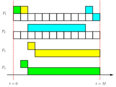
Fig. 2. Example of an optimal schedule on a heterogeneous platform, where a sending worker also receives a task.
3. General platforms
3.1. NP-completeness
workers into disjoint sets of senders and receivers. There exist situations where, to minimize the global makespan, it is useful that sending workers also receive tasks. Consider the following example. We have four workers (see Table 1 for their parameters). An optimal solution is shown in Figure 2, with a makespanM = 12: Workers P3 andP4 do not own any task, and they are computing very slowly. So each of them can compute exactly one task. WorkerP1, which is a fast processor and communicator, sends them their tasks and receives later another task from worker
P2 that it can compute just in time. Note that worker P1 is both sending and receiving tasks. Trying to solve the problem under the constraint that no worker also sends and receives, it is not feasible to achieve a makespan of 12. Worker P2 has to send one task either to worker P3 or to worker P4. Sending and receiving this task takes 9 time units. Consequently the processing of this task can not finish earlier than timet= 18.
Definition 1 (Scheduling Problem SP). Let N be a star-network with one special
processorP0called “master” andmworkers. Letnbe the number of identical tasks
distributed to the workers. For each workerPi, letLi be its initial number of tasks,
andwi be its computation time for one task. Each communication link, linki, has
an associated communication time ci for the transmission of one task. Finally let
T be a deadline. The decision problem of SP is: “Is it possible to redistribute the
tasks and to process them in timeT?”.
Theorem 1. SP is NP-complete in the strong sense.
For the proof we refer to the companion research report [5].
3.2. Polynomiality when computations are neglected
A major difficulty of the problem is the overlap of computation and the redistri-bution process. In this section we provide an optimal polynomial algorithm when neglecting the computations.
Without computations we get a classical data redistribution problem, where we can suppose that we already know the imbalance of the system. More precisely, we adopt the following abstract view of the new problem: themparticipating workers
P1, P2, . . . Pm hold their initial uniform tasksLi, 1 ≤i ≤m. For a workerPi the chosen algorithm for the computation of the imbalance has decided that the new load should beLi−δi. Ifδi>0, this means thatPiis overloaded and it has to send
δi tasks to some other processors. Ifδi <0,Pi is underloaded and it has to receive
−δi tasks from other workers. We have heterogeneous communication links and all sent tasks pass by the master. So the goal is to determine the order of senders and receivers to redistribute the tasks in minimal time.
Theorem 2. Knowing the imbalance δi of each processor, an optimal solution for
heterogeneous star-platforms is to order the senders by non-decreasingci-values and
the receivers by non-increasing order ofci-values.
Proof. To prove that the scheme described by Theorem 2 returns an optimal sched-ule, we take a scheduleS0 computed by this scheme. Then we take any other sched-uleS. We are going to transformSin two steps into our scheduleS0and prove that the makespans of the both schedules hold the following inequality: M(S0)≤M(S).
t t Pi0
Pi0+1
Pi0
Pi0+1
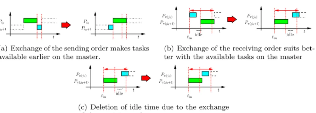
(a) Exchange of the sending order makes tasks available earlier on the master.
t t idlen idlen tin tin Pπ(j0) Pπ(j0+1) Pπ(j0) Pπ(j0+1)
(b) Exchange of the receiving order suits bet-ter with the available tasks on the masbet-ter
t t idle n tin tin Pπ(j0) Pπ(j0+1) Pπ(j0) Pπ(j0+1)
(c) Deletion of idle time due to the exchange of the receiving order.
Fig. 3. Schedule transformation.
In the first step we take a look at the senders. The sending from the master can not start before tasks are available on the master. We do not know the ordering of the senders in S but we know the ordering in S0: all senders are ordered in
non-decreasing order of theirci-values. Leti0 be the first task sent inS where the sender of task i0 has a biggerci-value than the sender of the (i0+ 1)-th task. We then exchange the senders of task i0 and task (i0+ 1) and call this new schedule
Snew. Obviously the reception time for the second task is still the same. But as you can see in Figure 3(a), the time when the first task is available on the master has changed: after the exchange, the first task is available earlier and ditto ready for reception. Hence this exchange improves the availability on the master (and reduces possible idle times for the receivers). We use this mechanism to transform the sending order ofS in the sending order of S0 and at each time the availability on the master is improved. Hence at the end of the transformation the makespan ofSnew is smaller than or equal to that ofS and the sending order ofSnew andS0 is the same.
In the second step of the transformation we take care of the receivers (cf. Fig-ures 3(b) and 3(c)). Having already changed the sending order of S by the first transformation ofSintoSnew, we start here directly by the transformation ofSnew. Using the same mechanism as for the senders, we call j0 the first task such that the receiver of taskj0 has a smaller ci-value than the receiver of task j0+ 1. We exchange the receivers of the tasksj0 andj0+ 1 and call the new scheduleSnew(1).
j0 is sent at the same time than previously, and the processor receiving it, receives it earlier than it received j0+1 in Snew. j0+1 is sent as soon as it is available on the master and as soon as the communication of task j0 is completed. The first of these two conditions had also to be satisfied by Snew. If the second condition is delaying the beginning of the sending of the task j0+ 1 from the master, then this communication ends at time tin+cπ0(j
0)+cπ0(j0+1) = tin+cπ(j0+1)+cπ(j0)
and this communication ends at the same time than under the schedule Snew ( here π(j0) (π0(j0)) denotes the receiver of task j0 in schedule Snew (Snew(1),
re-spectively)). Hence the finish time of the communication of taskj0+ 1 in schedule
Snew(1) is less than or equal to the finish time in the previous schedule. In all cases,
for the tasks received afterj0+1 except that we always perform the scheduled com-munications as soon as possible. Repeating the transformation for the rest of the schedule Snew we reduce all idle times in the receptions as far as possible. We get for the makespan of each schedule Snew(k): M(Snew(k))≤M(Snew) ≤M(S). As
after these (finite number of) transformations the order of the receivers will be in non-decreasing order of the ci-values, the receiver order ofSnew(∞) is the same as
the receiver order ofS0 and hence we haveS
new(∞) =S0. Finally we conclude that
the makespan of S0 is smaller than or equal to any other scheduleS and henceS0
is optimal.
4. An algorithm for scheduling on homogeneous star platforms: the best-balance algorithm
In this section we present the Best-Balance Algorithm (BBA), an algo-rithm to schedule on homogeneous star platforms. We use a bus network with communication speed c, but additionally we suppose that the computation powers are homogeneous as well. So we havewi=wfor alli, 1≤i≤m.
The idea of BBA is simple: in each iteration, we look if we could finish earlier if we redistribute a task. If so, we schedule the task, if not, we stop redistributing. The algorithm has polynomial run-time. It is a natural intuition that BBA is optimal on homogeneous platforms, but the formal proof is rather complicated.
4.1. Notations used in BBA
BBA schedules one task per iterationi. LetL(ki) denote the number of tasks of workerk after iteration i, i.e., afteri tasks were redistributed. The date at which the master has finished receiving the i-th task is denoted by m in(i). In the same way we call m out(i) the date at which the master has finished sending the i-th task. Let end(ki) be the date at which workerk would finish processing the load it would hold if exactly i tasks are redistributed. The worker k in iteration i with the biggest finish timeend(ki), who is chosen to send one task in the next iteration, is called sender. We call receiver the worker k with smallest finish time end(ki) in iterationiwho is chosen to receive one task in the next iteration.
In iterationi= 0 we are in the initial configuration: All workers own their initial tasksL(0)k =Lk and the makespan of each workerkis the time it needs to compute all its tasks: end(0)k =L(0)k ×w. m in(0) =m out(0)= 0.
4.2. The Best Balance Algorithm - BBA
We first sketch BBA:
In each iterationido: Compute the timeend(ki−1)it would take workerkto process
L(ki−1)tasks. A worker with the biggest finish timeend(ki−1)is arbitrarily chosen as sender, he is calledsender. Compute the temporary finish timesgend
(i)
k of each worker if it would receive fromsenderthei-th task. A worker with the smallest temporary finish time gend
(i)
with the same temporary finish time gend
(i)
k , we take the worker with the smallest finish timeend(ki−1). If the finish time ofsenderis strictly larger than the temporary finish timegend
(i)
senderofsender,sendersends one task toreceiverand iterate. Otherwise stop.
Lemma 1. On homogeneous star-platforms, in iterationithe Best-Balance
Al-gorithm(Algorithm 1) always chooses as receiver a worker which finishes
process-ing the first in iterationi−1.
Proof. As the platform is homogeneous, all communications take the same time and all computations take the same time. In Algorithm 1 the master chooses as receiver in iterationithe workerkthat would end the earliest the processing of the
i-th task sent. To prove that worker kis also the worker which finishes processing in iterationi−1 first, we have to consider two cases:
1. Task i arrives when all workers are still working.
As all workers are still working when the master finishes to send task i, the master chooses as receiver a worker which finishes processing the first, because this worker will also finish processing taskifirst, as we have homogeneous conditions. 2. Task i arrives when some workers have finished working.
If some workers have finished working when the master can finish to send task
i, all these workers could start processing taski at the same time. Our algorithm chooses in this case a worker which finished processing first.
In the following lemma we will show that schedules, where sending workers also receive tasks, can be transformed in a schedule where this effect does not appear. Lemma 2. On a platform with homogeneous communications, if there exists a
schedule S with makespanM, then there also exists a schedule S0 with a makespan
M0 ≤M such that no worker both sends and receives tasks.
Proof. We will prove that we can transform a schedule where senders might receive tasks in a schedule with equal or smaller makespan where senders do not receive any tasks.
If the master receives itsi-th task from processorPj and sends it to processor
Pk, we say thatPk receives this task from processorPj.
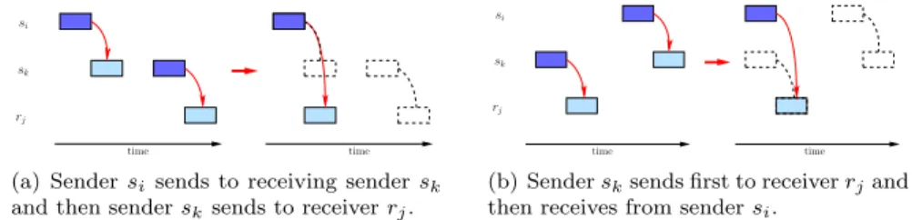
Whatever the schedule, if a sender receives a task we have the situation of a sending chain: at some step of the schedule a sendersi sends to a sender sk, while in another step of the schedule the sendersk sends to a receiverrj. So the master is occupied twice. As all receivers receive in fact their tasks from the master, it does not make a difference for them which sender sent the task to the master. So we can break up the sending chain in the following way: We look for the earliest time, when a sending worker, sk, receives a task from a sender, si. Let rj be a receiver that receives a task from sendersk. There are two possible situations:
1. Sender si sends to sender sk and later sender sk sends to receiver rj, see Fig-ure 4(a). This case is simple: As the communication from si to sk takes place first and we have homogeneous communication links, we can replace this commu-nication by an emission from sender si to receiver rj and just delete the second communication.
2. Sender sk sends to receiver rj and later sender si sends to sender sk, see Fig-ure 4(b). In this case the reception on receiverrj happens earlier than the emission of sendersi, so we can not use exactly the same mechanism as in the previous case. But we can use our hypothesis that sendersk is the first sender that receives a task. Therefore, sender si did not receive any task untilsk receives. So at the moment whensk sends torj, we know that sendersialready owns the task that it will send later to sender sk. As we use homogeneous communications, we can schedule the communicationsi→rj when the communicationsk →rj originally took place and delete the sending fromsi to sk.
As in both cases we gain in communication time, but we keep the same compu-tation time, we do not increase the makespan of the schedule, but we transformed it in a schedule with one less sending chain. By repeating this procedure for all send-ing chains, we transform the schedule S in a schedule S0 without sending chains while not increasing the makespan.
rj
si
sk
time time
(a) Sendersi sends to receiving sendersk
and then sendersksends to receiverrj. rj
si
sk
time time
(b) Sendersksends first to receiverrjand
then receives from sendersi.
Fig. 4. How to break up sending chains, dark colored communications are emissions, light colored communications represent receptions.
Proposition 1. Best-Balance Algorithm(Algorithm 1) calculates an optimal
schedule S on a homogeneous star network, where all tasks are initially located on
the workers and communication capabilities as well as computation capabilities are homogeneous and all tasks have the same size.
Proof. To prove that BBA is optimal, we take a schedule Salgo calculated by Algorithm 1. Then we take an optimal scheduleSopt. (Because of Lemma 2 we can assume that in the scheduleSoptno worker both sends and receives tasks.) We are going to transform by induction this optimal schedule into our scheduleSalgo.
As we use a homogeneous platform, all workers have the same communication time c. Without loss of generality, we can assume that both algorithms do all communications as soon as possible.So we can divide our scheduleSalgo insa steps andSoptinsosteps. A step corresponds to the emission of one task, and we number in this order the tasks sent. Accordingly thes-th task is the task sent during steps
and the actual schedule corresponds to the load distribution after thesfirst tasks. We start our schedule at timeT = 0.
LetS(i) denote the worker receiving thei-th task under scheduleS. Leti0 be the first step where Sopt differs from Salgo, i.e., Salgo(i0) 6=Sopt(i0) and∀i < i0,
Salgo(i) =Sopt(i). We look for a stepj > i0, if it exists, such thatSopt(j) =Salgo(i0) andj is minimal.
We are in the following situation: scheduleSoptand scheduleSalgoare the same for all tasks [1..(i0−1)]. As workerSalgo(i0) is chosen at stepi0, then, by definition
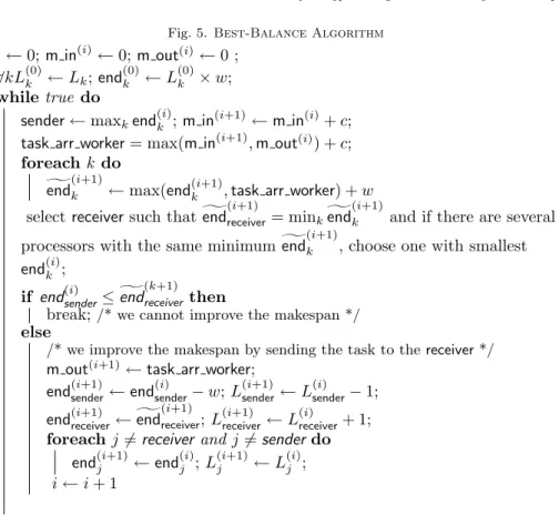
Fig. 5. Best-Balance Algorithm i←0;m in(i)←0;m out(i)←0 ; ∀kL(0)k ←Lk;end (0) k ←L (0) k ×w; whiletrue do
sender←maxkend (i) k ; m in
(i+1)
←m in(i)+c; task arr worker= max(m in(i+1),m out(i)) +c; foreachk do
g
end(ki+1)←max(end(ki+1),task arr worker) +w
selectreceiversuch thatendg
(i+1)
receiver = minkgend
(i+1)
k and if there are several processors with the same minimumgend
(i+1)
k , choose one with smallest end(ki);
if end(senderi) ≤endg
(k+1) receiver then
break;/* we cannot improve the makespan */
else
/* we improve the makespan by sending the task to thereceiver*/
m out(i+1)←task arr worker;
end(senderi+1)←end(senderi) −w;L(senderi+1)←L(senderi) −1; end(receiveri+1) ←gend
(i+1) receiver;L (i+1) receiver←L (i) receiver+ 1; foreachj 6=receiver andj6=senderdo
end(ji+1)←end(ji);L(ji+1)←L(ji);
i←i+ 1
of Algorithm 1, this means that this worker finishes first its processing after the reception of the (i0−1)-th tasks (cf. Lemma 1). AsSopt and Salgo differ in step
i0, we know thatSopt chooses workerSopt(i0) that finishes the schedule of its load after step (i0−1) no sooner than workerSalgo(i0).
Case 1: Let us first consider the case where there exists such a stepjSoSalgo(i0) =
Sopt(j) and j > i0. We know that worker Sopt(j) under schedule Sopt does not receive any task between stepi0 and stepj as j is chosen minimal.
We use the following notations for the scheduleSopt, depicted on Figures 6, 7, and 8:
Tj: the date at which the reception of task j is finished on worker Sopt(j), i.e.,
Tj =j×c+c (the time it takes the master to receive the first task plus the time it takes him to sendj tasks).
Ti0: the date at which the reception of task i0 is finished on workerSopt(i0), i.e., Ti0 =i0×c+c.
Fpred(j): time when computation of task pred(j) is finished, where task pred(j) denotes the last task which is computed on workerSopt(j) before taskjis computed. Fpred(i0): time when computation of taskpred(i0) is finished, where taskpred(i0)
com-puted.
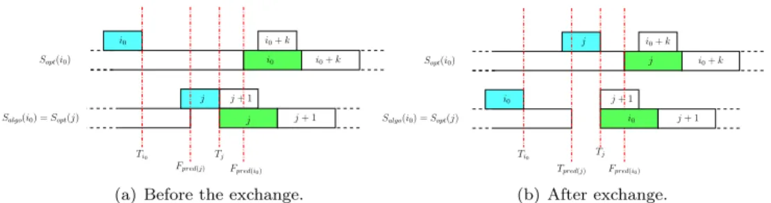
We have to consider two sub-cases: Tj≤Fpred(i0) (Figure 6(a)).
This means that we are in the following situation: the reception of taskjon worker
Sopt(j) has already finished when worker Sopt(i0) finishes the work it has been scheduled until stepi0−1.
In this case we exchange the tasksi0 andj of scheduleSopt and we create the following scheduleSopt0 :
Sopt0 (i0) =Sopt(j) =Salgo(i0),
Sopt0 (j) =Sopt(i0)
and ∀i 6= i0, j, Sopt0 (i) = Sopt(i). The schedule of the other workers is kept un-changed. All tasks are executed at the same date than previously (but maybe not on the same processor).
Sopt(i0) Salgo(i0) =Sopt(j) Ti0 Fpred(j) Tj Fpred(i0) j+ 1 i0 i0 j+ 1 i0+k j j i0+k i0
(a) Before the exchange.
Fpred(i0) Sopt(i0) Salgo(i0) =Sopt(j) Ti0 Tj Tpred(j) j j+ 1 i0 i0 j i0+k i0+k j+ 1 i0 (b) After exchange. Fig. 6. ScheduleSoptbefore and after exchange of tasksi0 andj.
Now we prove that this kind of exchange is possible.
We know that workerSopt(j) is not scheduled any task later than stepi0−1 and before stepj, by definition ofj. So we know that this worker can start processing task j when taskj has arrived and when it has finished processing its amount of work scheduled until step i0−1. We already know that workerSopt(j) =Salgo(i0) finishes processing its tasks scheduled until stepi0−1 at a time earlier than or equal to that of worker Sopt(i0) (cf. Lemma 1). As we are in homogeneous conditions, communications and processing of a task takes the same time on all processors. So we can exchange the destinations of steps i0 andj and keep the same moments of execution, as both tasks will arrive in time to be processed on the other worker: taski0will arrive at workerSopt(j) when it is still processing and the same for task
j on workerSopt(i0). Hence taski0 will be sent to workerSopt(j) =Salgo(i0) and workerSopt(i0) will receive taskj. So scheduleSoptand scheduleSalgo are the same for all tasks [1..i0] now. As both tasks arrive in time and can be executed instead of the other task, we do not change anything in the makespan M. And asSopt is optimal, we keep the optimal makespan.
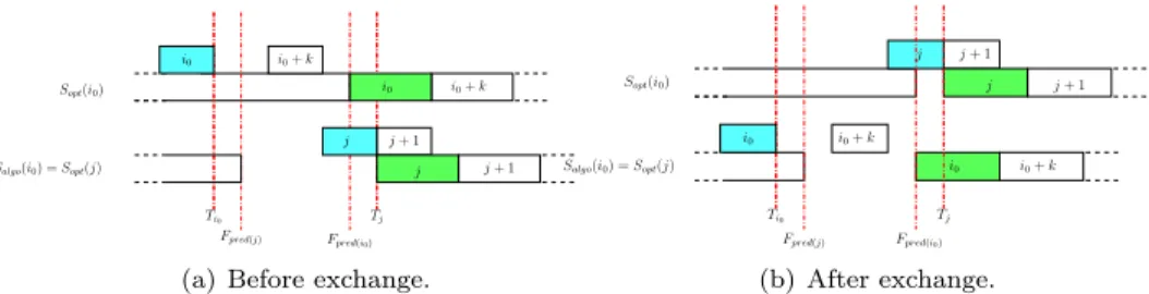
Tj≥Fpred(i0) (Figure 7(a)).
In this case we have the following situation: taskj arrives on workerSopt(j), when workerSopt(i0) has already finished processing its tasks scheduled until stepi0−1. In this case we exchange the schedule destinationsi0andjof scheduleSoptbeginning at tasksi0andj (see Figure 7). In other words we create a scheduleSopt0 :
∀i≥i0such thatSopt(i) =Sopt(i0): S0opt(i) =Sopt(j) =Salgo(i0)
∀i≥j such thatSopt(i) =Sopt(j): Sopt0 (i) =Sopt(i0)
and ∀i ≤ i0 Sopt0 (i) = Sopt(i). The schedule Sopt of the other workers is kept unchanged. We recompute the finish timesFS(s)
opt(j) of workersSopt(j) andSopt(i0)
for all stepss > i0.
Ti0 Fpred(j) Tj Fpred(i0) Salgo(i0) =Sopt(j) Sopt(i0) i0 i0+k i0 i0+k j j+ 1 j j+ 1
(a) Before exchange.
Tj Fpred(i0) Fpred(j) Ti0 Sopt(i0) Salgo(i0) =Sopt(j) i0 j+ 1 i0+k j i0 j j+ 1 i0+k i0 (b) After exchange. Fig. 7. ScheduleSoptbefore and after exchange of linesi0andj.
Now we prove that this kind of exchange is possible. First of all we know that worker Salgo(i0) is the same as the worker chosen in step j under schedule Sopt and so Salgo(i0) = Sopt(j). We also know that worker Sopt(j) is not scheduled any tasks later than step i0−1 and before stepj, by definition of j. Because of the choice of workerSalgo(i0) =Sopt(j) inSalgo, we know that workerSopt(j) has finished working when taskj arrives: at stepi0 workerSopt(j) finishes earlier than or at the same time as workerSopt(i0) (Lemma 1) and as we are in the case where
Tj ≥ Fpred(i0), Sopt(j) has also finished when j arrives. So we can exchange the
destinations of the workers Sopt(i0) andSopt(j) in the schedule steps equal to, or later than, stepi0 and process them at the same time as we would do on the other worker. As we have shown that we can start processing task j on workerSopt(i0) at the same time as we did on workerSopt(j), and the same for taski0, we keep the same makespan. And as Soptis optimal, we keep the optimal makespan.
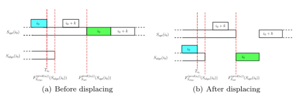
Case 2: If there does not exist aj, i.e., we can not find a schedule stepj > i0such that worker Salgo(i0) is scheduled a task under schedule Sopt, so we know that no other task will be scheduled on worker Salgo(i0) under the schedule Sopt. As our algorithm chooses in stepsthe worker that finishes tasks+1 the first, we know that workerSalgo(i0) finishes at a time earlier or equal to that ofSopt. WorkerSalgo(i0) will be idle in the scheduleSoptfor the rest of the algorithm, because otherwise we would have found a step j. As we are in homogeneous conditions, we can simply displace task i0 from worker Sopt(i0) to worker Salgo(i0) (see Figure 8). As we haveSopt(i0)6=Salgo(i0) and with Lemma 1 we know that workerSalgo(i0) finishes processing its tasks until stepi0−1 at a time earlier than or equal toSopt(i0), and we do not downgrade the execution time because we are in homogeneous conditions. Once we have done the exchange of taski0, the schedulesSoptandSalgo are the same for all tasks [1..i0]. We restart the transformation until Sopt =Salgo for all tasks [1..min(sa, so)] scheduled bySalgo.
Ti0 F(pred(i0)) Salgo (Salgo(i0)) F pred((i0)) Sopt (Sopt(i0)) Sopt(i0) Salgo(i0) i0 i0+k i0 i0+k i0
(a) Before displacing
Ti0 F(pred(i0)) Sopt (Sopt(i0)) Sopt(i0) Salgo(i0) F(pred(i0)) Salgo (Salgo(i0)) i0 i0+k i0+k i0 i0 (b) After displacing Fig. 8. ScheduleSoptbefore and after displacing taski0.
Now we will prove by contradiction that the number of tasks scheduled bySalgo,
sa, and Sopt, so, are the same. After min(sa, so) transformation steps Sopt=Salgo for all tasks [1..min(sa, so)] scheduled by Salgo. So if after these stepsSopt=Salgo for allntasks, both algorithms redistributed the same number of tasks and we have finished.
We now consider the casesa 6=so. In the case of sa> so,Salgo schedules more tasks thanSopt. At each step of our algorithm we do not increase the makespan. So if we do more steps thanSopt, this means that we scheduled some tasks without changing the global makespan. HenceSalgo is optimal.
Ifsa < so, this means that Sopt schedules more tasks than Salgo does. In this case, aftersatransformation steps,Soptstill schedules tasks. If we take a look at the schedule of the (sa+1)-th task inSopt: regardless which receiverSoptchooses, it will increase the makespan as we prove now. In the following we will callsalgothe worker our algorithm would have chosen to be the sender, ralgo the worker our algorithm would have chosen to be the receiver. sopt and ropt are the sender and receiver chosen by the optimal schedule. Indeed, in our algorithm we would have chosen
salgo as sender such that it is a worker which finishes last. So the time workersalgo finishes processing is Fsalgo =M(Salgo). Salgo chooses the receiverralgo such that
it finishes processing the received task the earliest of all possible receivers and such that it also finishes processing the receiving task at the same time or earlier than the sender would do. As Salgo did not decide to send the (sa+ 1)-th task, this means, that it could not find a receiver which fitted. Hence we know, regardless which receiver Sopt chooses, that the makespan will strictly increase (asSalgo =Sopt for all [1..sa]). We take a look at the makespan ofSalgo if we would have scheduled the (sa+1)-th task. We know that we can not decrease the makespan anymore, because in our algorithm we decided to keep the schedule unchanged. So after the emission of the (sa+ 1)-th task, the makespan would become M(Salgo) = Fralgo ≥Fsalgo.
AndFralgo ≤Fropt, because of the definition of receiver ralgo. As M(sopt)≥Fropt,
we have M(Salgo)≤M(Sopt). But we decided not to do this schedule asM(Salgo) is smaller before the schedule of the (sa+ 1)-th task than afterwards. Hence we get that M(Salgo)< M(Sopt). So the only possibility why Sopt sends the (sa+ 1)-th task and still be optimal is that, later on,roptsends a task to some other processor
rk. (Note that even if we chooseSoptto have no such chains in the beginning, some might have appeared because of our previous transformations). In the same manner as we transformed sending chains in Lemma 2, we can suppress this sending chain,
by sending task (sa+ 1) directly tork instead of sending to ropt. With the same argumentation, we do this by induction for all tasks k, (sa+ 1) ≤ k ≤ so, until schedule Sopt and Salgo have the same number so = sa and so Sopt = Salgo and henceM(Sopt) =M(Salgo).
Complexity: The initialization phase is in O(m), as we have to compute the finish times for each worker. The while loop can be run at maximum n times, as we can not redistribute more than the n tasks of the system. Each iteration is in the order ofO(m), which leads us to a total run time ofO(m×n).
5. Scheduling on platforms with homogeneous communication links and heterogeneous computation capacities
In this section we present an algorithm for star-platforms with homogeneous communications and heterogeneous workers, theMoore Based Algorithm(MBA). As the name says, this algorithm is based onMoore’s algorithm[6], [7], whose aim is to maximize the number of tasks to be processed in-time, i.e., before tasks exceed their deadlines. Moore’s algorithm gives a solution to the 1||P
Uj problem when the maximum number, amongntasks, has to be processed in time on a single machine. Each task k, 1 ≤k ≤ n, has a processing timewk and a deadline dk, before which it has to be processed.
For a given makespan, we compute if there exists a possible schedule to finish all work in time. If there is one, we optimize the makespan by a binary search.
5.1. Framework and notations for MBA
We keep the star network of Section with homogeneous communication links. In contrast to Section we suppose m heterogeneous workers who own initially a number Li of identical independent tasks.
LetM denote the objective makespan for the searched schedule σ and fi the time needed by workerito process its initial load. During the algorithm execution we divide all workers in two subsets, whereSis the set of senders (si∈Siffi> M) andRthe set of receivers (ri∈Riffi < M). As our algorithm is based on Moore’s, we need a notation for deadlines. Let d(rki)be the deadline to receive the k-th task
on receiver ri. lsi denotes the number of tasks sender i sends to the master and
lri stores the number of tasks receiver i is able to receive from the master. With
help of these values we can determine the total amount of tasks that must be sent asLsend=Psilsi. The total amount of tasks if all receivers receive the maximum
amount of tasks they are able to receive is Lrecv =Prilri. Finally, letLsched be
the maximal amount of tasks that can be scheduled by the algorithm.
5.2. Moore based algorithm - MBA
Principle of the algorithm: Considering the given makespan we determine overcharged workers, which can not finish all their tasks within this makespan. These overcharged workers will then send some tasks to undercharged workers, such that all of them can finish processing within the makespan. The algorithm solves the following two questions: Is there a possible schedule such that all workers
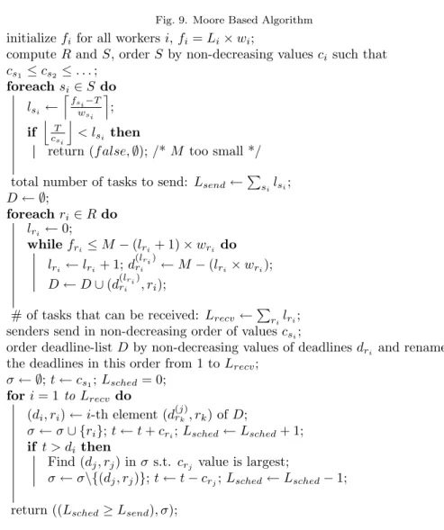
Fig. 9. Moore Based Algorithm
initializefifor all workers i,fi=Li×wi;
computeR andS, orderS by non-decreasing valuesci such that
cs1≤cs2 ≤. . .; foreachsi ∈S do lsi← lf si−T wsi m ; if jT csi k < lsi then
return (f alse,∅); /*M too small */ total number of tasks to send: Lsend←Psilsi;
D← ∅; foreachri∈R do lri←0; whilefri≤M −(lri+ 1)×wri do lri←lri+ 1;d (lri) ri ←M −(lri×wri); D←D∪(d(lri) ri , ri);
# of tasks that can be received: Lrecv ←Prilri;
senders send in non-decreasing order of valuescsi;
order deadline-listDby non-decreasing values of deadlinesdri and rename
the deadlines in this order from 1 toLrecv;
σ← ∅; t←cs1;Lsched= 0; fori= 1toLrecv do (di, ri)←i-th element (d (j) rk, rk) ofD; σ←σ∪ {ri};t←t+cri;Lsched←Lsched+ 1; if t > di then
Find (dj, rj) inσs.t. crj value is largest;
σ←σ\{(dj, rj)};t←t−crj;Lsched←Lsched−1;
return ((Lsched≥Lsend), σ);
can finish in the given makespan? In which order do we have to send and receive to obtain such a schedule?
The algorithm can be divided into four phases:
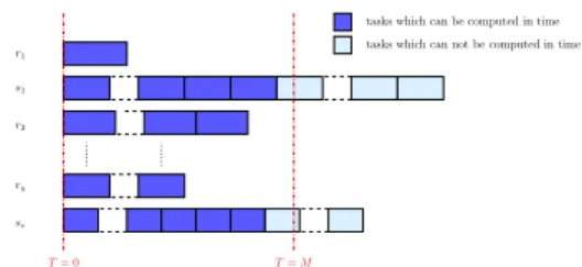
Phase 1 decides which of the workers will be senders and which receivers, depending of the given makespan (see Figure 10). Senders are workers which are not able to process all their initial tasks in time, whereas receivers are workers which could treat more tasks in the given makespanM than they hold initially.
Phase 2fixes how many transfers have to be scheduled from each sender such that the senders all finish their remaining tasks in time. Sendersi will have to send an amount of taskslsi =
lf si−T
wsi
m
(i.e., the number of light colored tasks of a sender in Figure 10).
T= 0 T=M r1 s1 r2 ru sv
tasks which can not be computed in time tasks which can be computed in time
Fig. 10. Initial distribution of the tasks to the workers.
receive, i.e., a pair (d(rij), rj) that denotes thei-th deadline of receiverrj. See Figure
11 for an example.
computation of initial tasksLri
Frj receiverrj T−1×wrj T−(lrj−1)×wrj T−lrj×wrj T−2×wrj M T= 0 d(lrj) rj d (lrj−1) rj d (1) rj d(2) rj
Fig. 11. Computation of the deadlinesd(rkj)for workerrj.
Phase 4is the proper scheduling step: The master decides which tasks have to be scheduled on which receivers and in which order. If the schedule is able to send at leastLsendtasks the algorithm succeeds, otherwise it fails.
Algorithm 2 describes MBA in pseudo-code. Note that the algorithm is written for heterogeneous conditions, but here we study it for homogeneous communication links.
Theorem 3. MBA (Algorithm 2) succeeds to build a scheduleσfor a given makespan
M, if and only if there exists a schedule with makespan less than or equal to M,
when the platform is made of one master, several workers with heterogeneous com-putation power but homogeneous communication capabilities.
Moore’s Algorithm constructs a maximal setσof early jobs on a single machine scheduling problem. In [5] we show that our algorithm can be reduced to this problem.
Proposition 2. Performing a binary search with precision = λ1, where λ =
lcm{βi, δi}, 1 ≤ i ≤ m, on Algorithm 2 returns in polynomial time an optimal
schedule σ for the following scheduling problem: minimizing the makespan on a
star-platform with homogeneous communication links and heterogeneous workers where the initial tasks are located on the workers.
For the proof we refer to the companion research report [5]. 6. Related work
To the best of our knowledge, there are no papers dealing with the same type of data redistribution algorithms which can be overlapped by computations (provided that enough data is available locally).
However, Redistribution algorithms have been well studied in the litera-ture. Unfortunately already simple redistribution problems are NP complete [8]. For this reason, optimal algorithms can be designed only for particular cases, as it
is done in [9]. In their research, the authors restrict the platform architecture to ring topologies, both uni-directional and bidirectional. In the homogeneous case, they were able to prove optimality, but the heterogenous case is still an open problem. In spite of this, other efficient algorithms have been proposed. For topologies like trees or hypercubes some results are presented in [10].
Theload balancing problemis not directly dealt with in this paper.
Any-way we want to quote some key references to this subject, as the results of these algorithms are the starting point for the redistribution process. Generally load bal-ancing techniques can be classified into two categories. Dynamic load balbal-ancing strategies and static load balancing. Dynamic techniques might use the past for the prediction of the future as it is the case in [11] or they suppose that the load varies permanently [12]. That is why for our problem static algorithms are more interesting: we are only treating star-platforms and as the amount of load to be treated is knowna priori we do not need prediction. For homogeneous platforms, the papers in [13] survey existing results. Heterogeneous solutions are presented in [14] or [15]. This last paper is about a dynamic load balancing method for data parallel applications, called theworking-manager method: the manager is sup-posed to use its idle time to process data itself. So the heuristic is simple: when the manager does not perform any control task it has to work, otherwise it schedules. 7. Conclusion
We have dealt with the problem of scheduling and redistributing independent and identical tasks on heterogeneous master-slave platforms. We have proved the NP completeness (in the strong sense) of the problem for fully heterogeneous plat-forms. We have also proved that this problem is polynomial when computations are negligible, which shows the additional complexity induced by the overlap be-tween communications and computations in the general case. Also, we were able to present optimal polynomial algorithms for special important topologies: a simple greedy algorithm for homogeneous star-networks, and a more complicated algorithm for platforms with homogeneous communication links and heterogeneous workers. The proof of optimality for both algorithms turned out rather complicated. On the more practical side, examples and simulations to compare the performance of the different algorithms are available in [5].
A natural extension of this work would be to derive approximation algorithms, i.e., heuristics whose worst-case is guaranteed within a certain factor to the optimal, for the fully heterogeneous case. However, it is often the case in scheduling problems for heterogeneous platforms that approximation ratios contain the quotient of the largest platform parameter by the smallest one, thereby leading to very pessimistic results in practical situations.
More generally, much work remains to be done along the same lines of load-balancing and redistributing while computation goes on. We can envision dynamic master-slave platforms whose characteristics vary over time, or even where new resources are enrolled temporarily in the execution. We can also deal with more complex interconnection networks, allowing slaves to circumvent the master and exchange data directly.
[1] BOINC: Berkeley Open Infrastructure for Network Computing. http://boinc. berkeley.edu.
[2] SETI. URL:http://setiathome.ssl.berkeley.edu.
[3] Einstein@Home. http://einstein.phys.usm.edu.
[4] M. R. Garey and D. S. Johnson. Computers and Intractability, a Guide to the
Theory of NP-Completeness. W.H. Freeman and Company, 1979.
[5] Loris Marchal, Veronika Rehn, Yves Robert, and Frdric Vivien. Scheduling and data redistribution strategies on star platforms. Research Report 2006-23, LIP, ENS Lyon, France, June 2006.
[6] Peter Brucker. Scheduling Algorithms. Springer-Verlag New York, Inc., Secaucus,
NJ, USA, 2004.
[7] J.M. Moore. An n job, one machine sequencing algorithm for minimizing the number
of late jobs. Management Science, 15(1), September 1968.
[8] U. Kremer. NP-Completeness of dynamic remapping. InProceedings of the Fourth
Workshop on Compilers for Parallel Computers, Delft, The Netherlands, 1993. also
available as Rice Technical Report CRPC-TR93330-S.
[9] H. Renard, Y. Robert, and F. Vivien. Data redistribution algorithms for heterogeneous processor rings. Research Report RR-2004-28, LIP, ENS Lyon, France, May 2004.
Available at the urlhttp://graal.ens-lyon.fr/∼yrobert.
[10] M-Y. Wu. On runtime parallel scheduling for processor load balancing. IEEE Trans.
Parallel and Distributed Systems, 8(2):173–186, 1997.
[11] M. Cierniak, M.J. Zaki, and W. Li. Customized dynamic load balancing for a network
of workstations.Journal of Parallel and Distributed Computing, 43:156–162, 1997.
[12] M. Hamdi and C.K. Lee. Dynamic load balancing of data parallel applications on a
distributed network. In9th International Conference on Supercomputing ICS’95,
pages 170–179. ACM Press, 1995.
[13] B. A. Shirazi, A. R. Hurson, and K. M. Kavi. Scheduling and load balancing in
parallel and distributed systems. IEEE Computer Science Press, 1995.
[14] M. Nibhanupudi and B. Szymanski. Bsp-based adaptive parallel processing. In
R. Buyya, editor,High Performance Cluster Computing. Volume 1: Architecture
and Systems, pages 702–721. Prentice-Hall, 1999.
[15] Alessandro Bevilacqua. A dynamic load balancing method on a heterogeneous cluster