Who Moves the Market?
A Study of Stock Prices and Sector Cashflows
*Brian Boyer
[email protected]
Lu Zheng
[email protected]
February, 2003
∗We would like to thank Sugato Bhattacharyya, Randolph Cohen, Kenneth French, William Goetzmann, Roger
Ibbotson, Grant McQueen, Tyler Shumway, Clemens Sialm, Rene Stulz, Paula Tkac, Vincent Warther, Toni Whited, and seminar participants at the University of Michigan Business School, Brigham Young University, and the American Finance Association meetings (2003) for useful comments. Contact information: Brian Boyer, Brigham Young University, Marriott School of Management, Provo UT, 84602-3313. Phone: 801-422-7641; email: [email protected]. Lu Zheng, University of Michigan Business School, 701 Tappan St., Ann Arbor, MI, 48109-1234. Phone: 734-763-5392; e-mail: [email protected].
Who Moves the Market?
A Study of Stock Prices and Sector Cashflows
Abstract
In this paper, we explore the relation between stock market returns and cash flows to the stock market from seven major investment sectors in the economy: Mutual Funds, Households, Pension Funds, Foreign Investors, Insurance Companies, Closed-end Funds, and Other institutional investors. Our goal is to address the following questions: 1) Do the return-cashflow relations differ across sectors? 2) Are the differences caused by distinct trading behaviors, such as positive feedback trading, or the fact that trades of specific sectors systematically impact the overall level of the market?
Using the Flow of Funds Accounts, we find that the quarterly contemporaneous relation between flow and return is positive and significant for Mutual Funds, Foreigners, Pension Funds and Insurance Companies. For example, over the entire sample we find that a one standard deviation realization in unexpected mutual fund flow corresponds with a 2.4 percent increase in the quarterly stock market return. We then develop a GMM framework to estimate higher frequency covariance measures based on a decomposition method developed in Sias, Starks and Titman (2001). We find that the positive contemporaneous quarterly covariance for Mutual Funds, Foreigners, and Insurance Companies is driven mainly by a strong contemporaneous monthly relation, suggesting that these sectors may exert price pressure on the market through their demand for stocks. The price impact appears to be temporary and is reversed in the subsequent months.
I. INTRODUCTION
Empirical evidence indicates that trading behaviors vary across broad investor groups, such as households and institutions. In asset pricing models with hetero-geneous agents, demand variables such as trading volume or fund flow can play an important role in determining asset prices.1 In this paper, we study the joint behav-ior of the aggregate stock market return and net cashflows to the stock market from different investor groups. Our goal is to gain a better empirical understanding of the impact investor heterogeneity may have on asset prices. Specifically, we are inter-ested in determining who is the marginal investor in the economy. If heterogeneous investors trade among themselves, whose behavior has significant price implications for the market portfolio?
Recent studies document that individuals and various types of institutions exhibit different trading behaviors. Del Guercio (1996)finds that prudence restrictions cause different types of institutions to make distinctive investment decisions. Cohen (1998) provides evidence that institutions and individuals differ in their asset allocation deci-sions. In addition, Dennis and Strickland (2002)find that individuals and institutions exhibit different trading behaviors on days of high market volatility.
Meanwhile, several studies find that trading by institutions in general may have important price effects on stocks. Badrinath, Kale and Noe (1995) and Sias and Starks (1997) relate institutional ownership to distinct lead-lag patterns in stock returns. Gompers and Metrick (2001)find that the increase in institutional ownership explains part of the disappearance of the historical small-company stock premium. Chakravarty (2000) provides evidence that institutional trades may impact stock prices because of superior information. Nofsinger and Sias (1999), Wermers (1999), 1For example, see Campbell and Kyle (1993), Campbell, Grossman and Wang (1993), Wang
Cai and Zheng (2000), Griffin, Harris and Topaloglu (2001), and Sias, Starks and Titman (2001) all document a strong positive contemporaneous relation between institutional trading and stock returns.
Other studies have focused primarily on determining whether flows into mutual funds have important market-wide price effects. Warther (1995) studies the relation between monthly flows into mutual funds and market returns from 1984 to 1993 and finds a significant contemporaneous relation between market returns and monthly mutual fundflows. Goetzmann and Massa (1998) examine the relation between daily flows of three Fidelity index funds and S&P 500 market returns from 1993 to 1998. Their results suggest that the market reacts to daily mutual fund demand. Edelen and Warner (2001) study the lead-lag relations between stock market returns and aggregate equity fundflows using dailyflow data and intra-day returns from February 1998 through June 1999. They document a positive concurrent daily relation and show that this concurrent relation is mainly caused by returns responding to flows.
In our study, aggregate net purchases of corporate equities are divided among seven major investment sectors in the economy: Mutual Funds, Households, Pension Funds, Foreign Investors, Insurance Companies, Closed-End Funds, and Other Institutions. Our data covers a broad sample of all investors in the economy and spans a long time period, from 1952 to 1995. We address the following questions: 1) Do the return-cashflow relations differ across the seven investor groups? 2) Are the differences caused by distinct trading behaviors, such as positive feedback trading, or the fact that trades of specific sectors systematically impact the overall level of the market? While distinct sector trading behaviors are interesting to observe, researchers, practi-tioners and policy makers are more concerned about whether certain sectors move the stock market. The findings of this paper will provide insights into the asset pricing models with heterogeneous agents and the growing literature of investor behavior. The empirical results will also help regulators form policies based on sector specific
price effects.
Using a simple correlation test and regression analysis, wefind that the quarterly contemporaneous relations between return and flow are positive and significant for Mutual Funds, Foreign Investors, and Pension Funds for the full sample period. In addition, the significant contemporaneous relations are mainly due to the unexpected component of cashflows. For example, over the entire sample we find that a one standard deviation realization in unexpected mutual fund flow (approximately $6.1 billion in 1995) corresponds with a 2.4 percent increase in the quarterly stock market return. Next, we divide our sample period into two subsample periods: 1952 to 1983 and 1984 to 1995. The two subsample periods differ in many aspects, for example, the percentage equity ownership by the sectors, stock market returns, cashflow volatility, etc. The later period also corresponds to the sample period in Warther (1995). When we study the quarterly contemporaneous relations for the two subsample periods, we find that the positive relations for Mutual Funds and Foreign Investors are stronger in the second subperiod. In addition, unexpected cashflows of Insurance Companies are positively and significantly related to stock market returns in the second subperiod. We identify three potential explanations for the positive contemporaneous relations between sector flows and stock market returns.
First, a sector may move market prices through “noninformational” or “liquidity” trades. “Noninformational” traders shift their demand curve for exogenous reasons. Other investors are willing to accommodate these trades only if there are price con-cessions since they are risk averse and are pushed away from their preferred portfolio positions. This explanation is consistent with models developed by Grossman and Miller (1988), Stoll (1978), Campbell, Grossman and Wang (1993), and Wang (1993a, 1993b). Cashflows reflect changes in demand. Hence, cashflows of market movers (those who initiate trades) should be positively correlated with market returns. On the other hand, cashflows of passive investors (liquidity providers or market
mak-ers) may be negatively correlated or uncorrelated with market returns, depending on whether price concessions are required to induce them to trade. Moreover, mod-els with heterogeneous investors suggest that the price impact of “noninformational” trades will tend to be reversed subsequently to reflect the change in expected returns due to previous price concessions(Campbell, Grossman and Wang 1993 and Wang 1993a). Hence, at higher frequencies, we may expect flows of “noninformational” market movers and subsequent returns to be negatively correlated.
Second, a sector may move the market if it has superior information relative to other sectors and if information revealed through trading drives price changes (French and Roll, 1986; Barclay, Litzenberger, and Warner, 1990). This explanation is consistent with the models developed by Copeland and Galai (1983), Kyle (1985), Glosten and Milgrom (1985), Campbell, Grossman and Wang (1993), Wang (1993a, 1993b), Foster and Viswanathan (1996), and Back, Cao, and Willard (2000). In this case, we should also observe a positive contemporaneous relation between the sector flows of market movers and market returns. At higher frequencies however, the relation betweenflows of market movers and subsequent returns should be zero or positive as stock prices may continue to incorporate new information. Chakravarty (2000) and Sias, Starks and Titman (2001) find evidence supporting informed trading on individual stocks by institutional investors.
Finally, the positive relation betweenflows and returns may be due to intra-quarter positive feedback trading. Warther (1995) finds no evidence of positive feedback trading for mutual funds at a monthly frequency. On the other hand, Edelen and Warner (2001) find some evidence that daily flows into mutual funds respond to lagged returns. However, using intra-day returns, they conclude that the positive contemporaneous daily relation betweenflows and returns is mostly caused by return responding toflow within the day. If sectorflow chases returns, we may again observe a positive contemporaneous relation betweenflows and returns using lower frequency
data. At higher frequencies however, the relation between returns and subsequent flows should be positive while the relation betweenflow and subsequent returns should be zero.
We estimate higher frequency lead-lag comovements in order to determine whether trades by the identified sectors do in fact have market-wide price impacts. The unfor-tunate drawback of our sectorflow data is its low quarterly frequency. As a result, we are limited to observing quarterly relations betweenflow and returns and are unable to observe within quarter dynamics directly. Hence, to explore theflow-return dynamics within a quarter, we apply a covariance partitioning method developed in Sias, Starks and Titman (2001). The method allows us to utilize the higher frequency return data and decompose the quarterly covariances into components to estimate how much of the covariance arises from contemporaneous, lead, and lag cashflow-return relations respectively within a quarter. In this paper, we develop an estimation framework based on Hansen’s (1982) Generalized Method of Moments (GMM) which makes effi -cient use of the data and also provides robust standard errors of the higher-frequency covariance estimates. Applying this method, wefind that the monthly contemporane-ous covariances are positive and significant for Mutual Funds and Foreign Investors. The monthly contemporaneous covariance is also positive and significant for Pension Funds during 1952-1983 and for Insurance Companies during 1984-1995. In addition, we find no evidence of positive feedback trading for any sector. In fact, for Mutual Funds we find that the monthly relation between returns and subsequent flows is significantly negative. This result is consistent with findings of mutual fund flows in Warther (1995). We also find a reversal in prices following the mutual fund, foreign and insurance flows, consistent with the price pattern of “noninformational” trades. Thus, our results suggest that the demand shocks of these sectors may exert tem-porary price pressure on the market and that such effects are stronger in the second subperiod of our data.
Positive feedback trading may occur at intervals less than a month. Consequently, the positive relations we document should be viewed as an upper bound of the actual price impact of the sectorflows. However, the results of Goetzmann and Massa (1998) and Edelen and Warner (2001) who study dailyflows into mutual funds suggest that market returns respond to flows. Our results are therefore consistent with previous findings for mutual funds using higher frequency data. In addition, we also find that the cashflow-return relation for Foreign Investors is very similar to that for Mutual Funds. We interpret this result as interesting evidence that foreigners may also frequently play the role of marginal investor in the U.S. stock market. Meanwhile, flows from Insurance Companies and Pension Funds display some effects on the market during specific time periods. On the other hand, results for Households, Closed-end Funds, and Other Institutions do not indicate that trades by these sectors have systematic market-wide price effects.
We then decompose realized returns to examine which component of returns drives the positive contemporaneous correlations. Following Campbell (1991), Campbell and Shiller (1988a, 1988b), realized stock returns are decomposed into expected returns, dividend news, and future return news. A positive correlation between stock returns and news about future dividends does not reflect the change in price as a response to a demand shock but rather may reflect a change in cashflow in response to a supply shock of future dividends. If the positive correlation is due to demand shocks, it should reflect a negative correlation between flows and future return news. That is, if prices are discounted future dividends, and positive (negative)flows drive prices up (down) while dividends remain unchanged, then total returns at some point in the future must be lower (higher). The test results indicate thatflows of Mutual Funds, Foreign Investors, and Insurance Companies negatively comove with contemporaneous news about future expected returns. We interpret these results as further evidence that Mutual Funds, Foreign Investors and Insurance Companies are market movers.
Overall, our empirical results indicate that trades of Mutual Funds, Foreign In-vestors and Insurance Companies exert price pressure on the market. Nevertheless, the price impact appears to be temporary and is reversed in the subsequent months. The rest of the paper is organized as follows: Section II discusses data and institu-tional history. Section III describes the methodologies and empirical results. Section IV concludes.
II. DATA
A. Sources of Data
The primary data source for this study is the Flow of Funds Accounts, issued by the Board of Governors of the Federal Reserve System. TheFlow of Funds Accounts records holdings and purchases of major assets by sectors in the U.S. economy starting in 1952. In our analyses, we use the end-of-quarter holdings and quarterly net pur-chases of equities for seven major investment sectors: Mutual Funds, Households and Non-profit Organizations, Pension Funds, Foreign Investors, Insurance Companies, Closed-End Funds, and Other Institutions. This study covers a 44-year time period, from the first quarter of 1952 through the last quarter of 1995. The net purchases of equity is a more direct measure of investment in the equity market than money flow into equity mutual funds as used in the fundflow literature, because purchases or sales of fund shares do not perfectly correspond to purchases or redemptions of equity investment.
Researchers have used several different data sources to analyze the flow-return relation. Most papers on institutional trading and stock returns use the Spectrum quarterly institutional holdings data based on the 13F filings with the SEC.2 The 2For example, Badrinath, Kale and Noe (1995), Cai, Kaul and Zheng (2001), Gompers and
Spectrum data provides information on institutional holdings of individual stocks. The price effect documented in these studies are driven by the concentration of large trades in an individual stock. Such a price effect could be idiosyncratic and bear no relation to market returns. Different types of institutional investors have been studied using the Spectrum definitions of manager types.3 However, these categorizations are noisy and problematic as pointed out by Gompers and Metrick (2001). Warther (1995, 1998) uses monthly mutual fund flow data provided by Investment Company Institute and focuses on the market return-flow relation of the mutual fund sector. Goetzmann and Massa (1998) and Edelen and Warner (2001) use high frequency dailyflows and thus are able to address the lead-lag relation betweenflow and market returns. Nevertheless, the high frequency data sets can not address the issue of long run effects as they cover a short sample period of a less broad sample.
Using theFlow of Funds Accounts, we analyze a broad sample including all major investment sectors for a long sample period of 44 years. The data we use is similar in spirit to the ICI mutual fundflow data used in Warther (1995, 1998), but for a broader sample including various investment sectors. The relatively clean classifications of investor types allow us to examine the differences in the market return-flow relations across sectors and identify the potential marginal investors in the economy. Test results using this broad sample should provide us with better understanding of the heterogeneity of the cashflow-market return relations for various investor groups in the US economy. In fact, conclusions drawn without considering all investment sectors of the economy only tell a partial story.
The Flow of Funds Accounts data allows us to study the return-flow dynamics of foreign investors separately. The foreign investor sector is usually excluded or
use the Spectrum holdings of institutions. Wermers (1999) uses the Spectrum holdings of individual mutual funds.
bundled together with individual investors in the literature. On the other hand, academics have argued that foreign investors display distinct trading behavior and effects. For instance, Tesar and Werner (1995) document high turnover rate on foreign equity investments relative to turnover on domestic equity markets. Choe, Kho and Stulz (1999) study the possible destabilizing effect of foreign investor on stock prices in Korea. Dornbusch and Park (1995) argue that foreign investors follow positive feedback strategies and cause stock prices to overreact to changes in fundamentals. Boyer, Kuamgai, and Yuan (2001) provide evidence that international stock market crises are spread by the trading behavior of investors rather than fundamentals. Froot, O’Connell and Seasholes (2001) document positive feedback trading as well as price impact by international investors. Thus, it is important to study the return-flow relation of foreign investors separately.
The limitation of the Flow of Funds Accounts is its low frequency. Like the Spec-trum data, the Flow of Funds Accountsreport holdings and net purchases on a quar-terly basis. The issue of intra-quarter lead-lag relation of flow and return is thus difficult to address. To mitigate the problem, we use a covariance decomposition method developed in Sias, Starks, Titman (2001) in a GMM framework to estimate, how much of the covariance arises from contemporaneous, lead and lag cashfl ow-return relations within the quarter. We also decompose the realized ow-returns following Campbell and Shiller (1988a,b) and Campbell (1991) to further explore the source of the cashflow-return relation.
The Appendix documents the original data sources for each of the seven investment sectors. Data for the Flow of Funds Accountscome from a variety of government and nongovernment sources. Many of the data are published. Some are available to the public upon request. Others such as those gathered from individual depository-institution financial reports are obtained from internal data bases maintained by offices within the Federal Reserve System.
The market returns are the total returns on the value-weighted CRSP stock port-folio. The interest rate variable is the three-month nominal risk free rate from CRSP. Dividend price ratios are also obtained from CRSP. Other macro-economic variables are provided by Ibbotson Associates.
B. A Historical Look at the Players in the Market
Figure 1 shows the percentage equity holdings of the major investment sectors for 1952 through 1995. The clear trend of ownership composition from 1952 to 1995 is the gradual increase in institutional stock holdings and the decrease in direct indi-vidual stock holdings. In 1952, Households held 91 percent of the equity market; Mutual Funds and Pension Funds together constituted only 3 percent of the market. During the recent four decades, Mutual Funds, Pension Funds, Insurance Companies, Other Financial Institutions, and Foreign Investors have all increased their equity stakes. The fastest-expanding sector over the whole period is Pension Funds, which grew from 1 percent in 1952 to 22 percent in 1995. The fast growth of pension fund equity holdings occurred from 1952 through 1985. In the 1990s, the dramatic ex-pansion of mutual fund equity holdings took place. Mutual funds increased their equity ownership from 6 percent of the overall equity market in 1990 to 13 percent in 1995.4Although Households, including nonprofit organizations, are still the major players in the equity market, they have been the net sellers of equity in the eighties 4The mutual fund industry first appeared in the United States in the 1924 and grew steadily
during the decades after World War II. Driven by the bull market in the 1960s, equity mutual funds more than tripled their assets, and bond mutual funds almost doubled theirs. However, there was little growth of equity funds in the 1970s because of the severe bear market caused by high inflation during the middle years of the decade. Along with the stock market, the mutual fund industry rebounded strongly in the 1980s, with steady cash inflow and an emergence of many new funds. In the 1990s, mutual funds, especially equity mutual funds, experienced an expansion in asset size and number of mutual fund share holders.
and nineties. Consequently, they directly owned 52 percent of the market in 1995. This decline in direct holdings of stocks by individuals has been offset by an increase in indirect holdings through such vehicles as pension plans and mutual funds.
Figure 1 also shows a sharp decline in equity holdings for Households and a sharp increase in equity holdings for Other Institutions during the first quarter of 1969. This spike is due to a change in the classification of equity holdings by Bank Personal Trusts. These were initially included under the Household sector but were counted in the Other Institutions sector beginning in 1969.5
Cohen (1998) uses the Flow of Funds Accounts to compare the asset allocation decision between equity and debt of individuals and institutions. He focuses on the asset allocation decision process of the two types of investors. For this purpose, he defines “individual” and “institution” based on whether the allocation decision is made by the security holder or a fund manager: individual, mutual funds and defined contribution plans are counted as household holdings and pension funds, banks, and insurance companies are counted as “institutions”. In our paper, we study the price impact and the return-chasing pattern of different sectors in the equity market. We form our sectors based on investment objectives,fiduciary responsibilities and information that can lead to different patterns and impact of trading. The primary variable analyzed in Cohen (1998) is the relative level of equity and debt investment for each sector, while our variable of interest is flows into equity market through different sectors. Unlike Cohen (1998), we do not study the interaction between the equity and the debt market.
5Personal communication with staff at the Board of Governors of the Federal Reserve System.
For our empirical tests, we checked to make sure that the results are not driven by this data reclassification.
III. METHODOLOGY AND EMPIRICAL RESULTS
A. Quarterly cashflows and Stock Returns
1. Summary Statistics.–
We first study the quarterly contemporaneous relations between sector cashflows and stock market returns. The time series of flow data span 44 years. The measure of cashflow for sector iin quarter t is defined as the net purchase of stocks for sector
i in quarter t divided by the total level of stock holdings of all sectors at the end of quarter t−1. This normalization measures new money relative to the total equity market capitalization and thus takes into account the overall price level of the equity market. It makes the time-series and cross-sectional sector observations comparable:
cashf lowt = (N et P urchase)t/(T otal Level)t−1. (1) Note that the sectorflows should add up to zero, after adjusting for the new issuance or buyback of stocks, which is only a small fraction of the equity market. Alterna-tively, we defineflow as the net purchase of stocks for sectoriin quartert divided by the total level of stock holdings of sectori at the end of quartert−1. All test results are qualitatively similar. In the paper, we report test results based on the cashflow definition in equation (1). The return series used is the value-weighted market port-folio from CRSP. The test results remain very similar when we use returns excluding dividends. We have additionally run all our tests using the excess return over the risk-free rate where the risk-free rate is the 3-month T-bill rate from CRSP. All results are again found to be quantitatively similar. In this paper, we report results using the total nominal return.
In Table I, we report summary statistics for the market return and sector flow data. Panel A reports summary statistics for the entire sample from the second
quarter of 1956 to the fourth quarter of 1995.6 The sample contains 175 quarters. The mean normalizedflow is positive for all sectors except for Households and Closed-End Funds. Pension Funds have the highest mean normalized flow at 0.19 percent followed by Mutual Funds at 0.07 percent. Theflow standard deviation is highest for Households at 0.40 percent and lowest for Closed-End Funds at 0.05 percent. Panel A also reports the correlations between the sectorflows. The sectorflows do not appear to be highly correlated. The highest correlation in Panel A of Table I is that between Pension Funds and Insurance Companies (0.189).
In Table I and throughout the paper, we divide our sample period into two sub-sample periods. These two subperiods are from 1952 to 1983 and from 1984 to 1995. The later period corresponds to the fast growth of the mutual fund industry and the sample period in Warther (1995). Dividing the sample in this manner allows us to compare our results across the two periods. The mean normalized cashflow for Mutual Funds is ten-times higher in the second subperiod than in the first subperiod, 0.203 percent versus 0.025 percent, reflecting the rapid growth of the mutual fund industry over the second subperiod. The mean Household normalizedflow is about four-times more negative in the second subperiod, -0.632 percent versus -0.149 percent, reflecting the general pattern of Households decreasing their direct stockholding and increasing their stockholding through mutual funds. There is also a rather large difference in the normalizedflows across the two periods for the sector of Other Institutions, 0.001 versus -0.103 percent. The normalized flow of Foreign Investors, Insurance Compa-nies, Pension Funds and Closed-End Funds appear to be comparable across the two periods. The mean quarterly total cashflow across all sectors is close to zero in the first subperiod, indicating an approximately fixed supply of stocks. In the second subperiod however, the mean quarterly total cashflow across all sectors is -0.29 per-cent, probably reflecting the fact that corporate America issued substantial amounts
of debt and retired equity during the 1980’s. In addition, note that the standard deviation of flow is much higher for all sectors in the second subperiod than in the first, except for Closed-End Funds. Hence, another reason for splitting up the sample is to ensure that the results are not an aberration caused by nonstationarity in the data.
2. Contemporaneous Relations.–
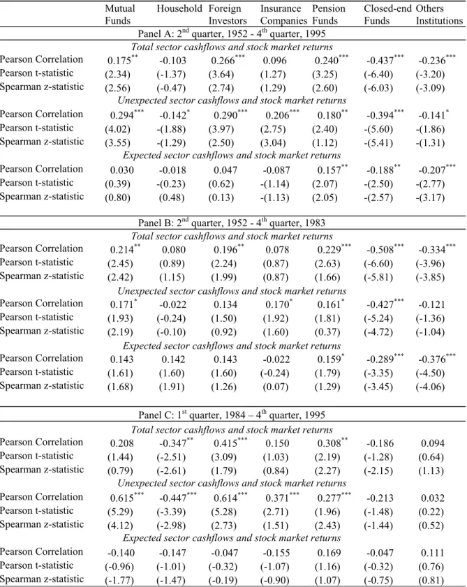
Table II reports correlations between sector cashflows and stock market returns for each of the seven sectors. We decompose total flows into expected flows and unexpected flows using the VAR model that we describe in the next section. The expected flows are the forecasts of the VAR model, and the unexpected flows are the residuals of the model. The decomposition allows us to learn about the possible difference in how stock market returns relate to predictable versus unpredictable com-ponents of sectorflows. We report the correlations of stock market returns with total cashflows, expected cashflows, and unexpected cashflows for each sector respectively. In this table, we use both the standard Pearson estimate and the Spearman rank test. Since Spearman’s method is based on ranks and is not sensitive to outliers and non-normality, it minimizes the effect of outliers on the test.
In Panel A, which reports results for the entire sample period, cashflows of Mu-tual Funds, Foreign Investors, and Pension Funds are significantly and positively correlated with stock market returns. The correlations are negative for Households, Closed-End Funds and Other Institutions. As seen from the table, the results are robust to both the parametric and non-parametric correlation tests. A negative cor-relation indicates that the sector is a residual trader of the stock market or that it follows contrarian strategies. A lack of correlation suggests that the sector does not have systematic price impact on the stock market. We are particularly interested in examining the sectors of which cashflows display positive correlations with the stock
market returns, because these sectors can potentially affect stock prices. However, as discussed above, a positive correlation is consistent with 1) “noninformational” sec-tor demand affecting stock prices; 2) sectors having superior information and timing their trades 3) sectors following positive feedback trading strategies. We will devote much effort in exploring the source of the positive correlations later in the paper. As we see from the correlations of the decomposed flows with returns, the results for the total flows are mainly driven by the unexpected flow component for Mutual Funds, Foreign Investors and Pension Funds. In addition, the unexpectedflows of Insurance Companies are also positively and significantly correlated with market returns.
Panel B and C report correlation statistics for the subsample periods. These results suggest that the positive correlations between the stock market returns and unex-pected flows are higher both in magnitude and in significance for Mutual Funds and Foreign Investors in the later period. This finding is consistent with the hypothesis that these sectors affect stock prices and that their effects are more pervasive during the later period in which they play a more important role in the equity market.
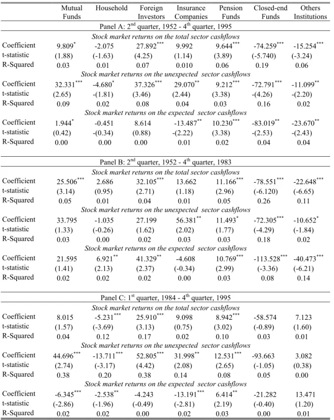
In Table III, we report estimated regression coefficients of stock market returns on the time series of seven sector cashflows using OLS. Numbers in parenthesis are t-statistics. Standard errors are calculated using the approach of Newey and West (1987) assuming the error structure is possibly autocorrelated up to eight lags. The findings are consistent with those of Table II. Cashflows of Mutual Funds, Foreign Investors and Pension Funds are positively related to stock market returns, and the results are driven mainly by the unexpected flow components. Unexpected flows of Insurance Companies are also positively correlated with market returns.
Using the summary statistics from Table I and the regression coefficients of Table III, we can get an idea of the economic significance of the cashflow-return relations. For example, the coefficient for total mutual fund flow reported in Panel A of Table III is approximately 9.8, implying that a one standard deviation realization in
nor-malized mutual fund flow (0.142 percent or $11.8 billion in 1995) corresponds with a 1.39 percent increase in the quarterly stock market return. The coefficient on For-eign Investors is approximately 27.9 implying a one standard deviation realization in normalized foreign flow (0.076 percent or $6.3 billion in 1995) corresponds with a 2.12 percent increase in the quarterly return. Using the results for unexpected flow in Panel A, the coefficient on mutual funds is approximately 32.3 implying a one standard deviation realization in unexpected mutual fund flow (0.073 percent or $6.1 billion in 1995)7 corresponds with a 2.4 percent increase in the quarterly stock market return, while for Foreign Investors, the coefficient is approximately 37.3 implying a one standard deviation realization in unexpected foreign flow (0.062 percent or $5.2 billion in 1995) is associated with a 2.3 percent increase in the quarterly market re-turn. Since Edelen and Warner (2001) have found some evidence that flows follow market returns, the positive relations we document should be viewed as an upper bound of the actual price impact of the sector flows. It is interesting to note that the cashflow-return relation for Foreign Investors is as strong, if not stronger than that for Mutual Funds and Pension Funds, despite the disproportionate attention and coverage given to these sectors by academics and the popular press. Thisfinding is consistent with the evidence in Froot, O’Connell and Seasholes (2001) that the sensitivity of local stock prices to foreign inflows is positive and large.
In the second subsample period, we observe higher regression coefficients for Mutual Funds and Foreign Investors using unexpectedflow than in thefirst subsample period. It is also interesting to note the difference in R-squared across the different subsamples for the unexpected flow regressions. In thefirst subsample, unexpected mutual fund flow explains a mere 2.9 percent of the return variance while unexpected foreignflow explains only 1.8 percent. In the second subsample however, the unexpectedflows for mutual funds and foreigners both explain about 38 percent of the variance in returns.
The relations between flows and returns for Mutual Funds and Foreign Investors are found to be stronger during the later period in which their equity holdings are larger and they trade perhaps more actively. For Pension Funds, the regression coefficients using unexpected flow are similar across the two periods, 11.5 versus 12.5, and the R-squared using unexpectedflow is only slightly higher during the second period, 0.03 versus 0.08. For Insurance Companies, the magnitude of the regression coefficients using unexpected flow is higher in the first subperiod and the significance levels are similar across the two periods.
We also examine the contemporaenous relations betweenflow and return controlling for changes in aggregate supply of stocks, where supply is measured as the quarterly total cashflow across all sectors. When we include the changes in aggregate stock supply as a control variable in the regressions, the results reported in Table III stay virtually unchanged. Hence, the positive contemporaneous relations between sector flows and stock returns are due to demand rather than supply shocks.
In summary, we find evidence that cashflows of Mutual Funds, Foreign Investors, Pension Funds and unexpected cashflows of Insurance Companies are positively cor-related with stock market returns. These relations are found to be stronger over the second subperiod for Mutual Funds and Foreign Investors. Subsections B and C are devoted to understanding the source of these positive correlations.
2. VAR Model.–
We use a VAR approach to study the lead-lag relations between quarterly sector cashflows and stock returns. Letyt+1 be ak×1 vector of variables observed at time
t+ 1 or earlier that help forecast future returns andflows. The vectoryt+1 is assumed to follow a first-order VAR
yt+1 =Ayt+wt+1. (2)
Since a higher order VAR can always be stacked into a first-order rendition, the first-order assumption is not restrictive. We use the Bayesian Information Crite-rion (BIC) and an analysis of the residuals to select the appropriate lag structure. The variables included in yt+1 are the quarterly market return, the quarterly sector
flows, the dividend-price ratio, the ‘relative’ short term interest rate, and a constant to estimate the intercept. Since sector flows approximately sum to zero, flows for Other Institutions are excluded from the set of explanatory variables as a precaution against multicollinearity. The dividend-price ratio is used following Fama French (1988) and Campbell and Shiller (1988a,b). If prices are discounted future dividends, then changes in the dividend price ratio should reflect changes in future expected returns. The variable is measured as total dividends paid over the previous year divided by the current stock price. The ‘relative’ short term interest rate is used be-cause many authors, including Fama and Schwert (1977) and Campbell (1987) have found that the short term interest rate helps forecast returns. This variable is mea-sured as the difference between the three month risk-free rate from CRSP and its one-year backward moving average. These measures for the dividend price ratio and the relative short term interest rate are discussed in Campbell (1991).
The parameters of (2) are estimated by OLS with standard errors calculated using the approach of Newey and West (1987) assuming the error structure is possibly autocorrelated up to eight lags. Hence, the standard errors are consistent even in the presence of heteroscedasticity and autocorrelation. We make no further assumptions about the nature of the error terms. Consistency of parameter estimates only requires thatyt+1 be stationary. Stationary tests of each series based on the unit root tests of Dickey-Fuller reject the null hypothesis that the time series is non-stationary at the one percent level. Using BIC and an analysis of the residuals to select the appropriate lag structure, we select a model with two lags. Results using additional lags are qualitatively similar. The model is estimated using all data in our sample from 1956
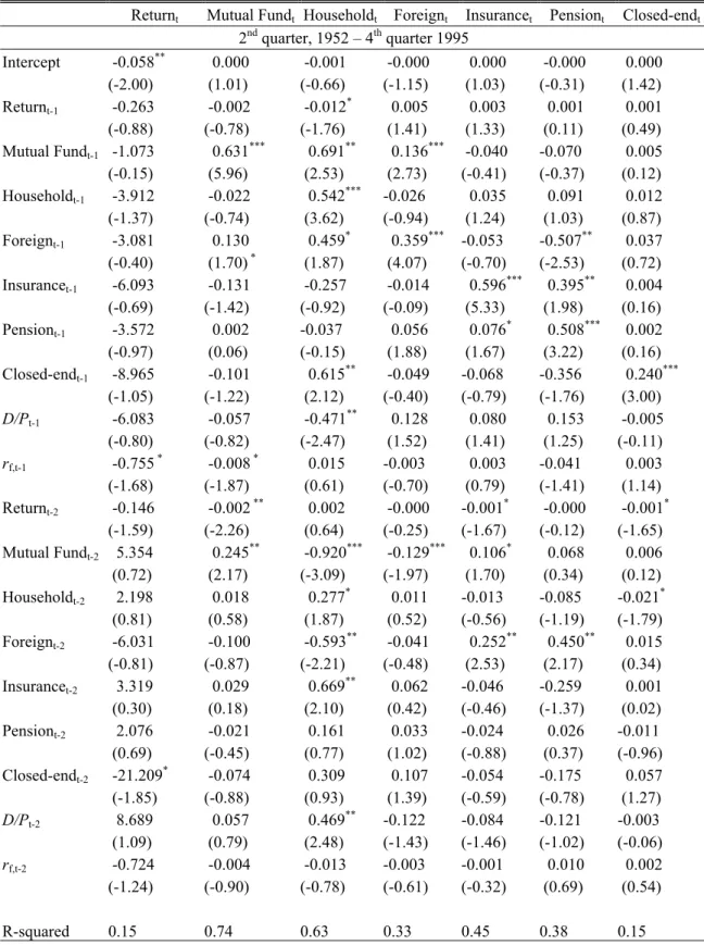
to1995, as well as over the two subperiods from 1956 to 1983 and from 1983 to 1995. Table IV reports the VAR coefficients for the entire sample. All sectorflows appear to be positively autocorrelated. However, we do not find much evidence for cross effects between sector flows. In addition, we find no significant relation between returns and lagged cashflows or between cashflows and lagged returns on a quarterly basis, except that mutual fund flows are negatively correlated with the two-quarter lagged return. Using a Wald test to study the Granger-causality between stock market returns and sector cashflows, wefind no evidence that stock market returns Granger cause any of the sector cashflows or that cashflows of any sector Granger cause returns. Given the lack of a significant lead-lag relation between quarterlyflows and returns, this result is not surprising. Any lead-lag effects among these variables are likely to be carried out very quickly and therefore difficult to detect using quarterly data. To get a better sense of the cause-effect relationship, higher frequency data is needed. We explore methods of estimating higher frequency covariances in the next section.
In addition to the lagged returns and cashflows, other variables may also be corre-lated with market returns and cashflows.8 Omitting such variables may cause some misleading results since lagged returns and cashflows may just be proxies for other factors. We check the robustness of our VAR results by adding five variables which reflect economic and demographic conditions. The variables are: population me-dian age, meme-dian family income and inflation. We find that the magnitude of the coefficients changes very little when we add these conditioning variables.
8For example, a number of papers, including Rozeff (1984), Campbell and Shiller (1988a, b),
Fama and French (1988) and Bekaert and Hodrick (1992) document some evidence that dividend yields are positively correlated with future stock returns. Bakshi and Chen (1994) suggests that a rise in average age predicts a rise in risk premiums.
B. A Time Decomposition of Covariance
Given that we have found positive correlations between quarterly cashflows and quarterly market returns for some sectors, we now investigate the cause-effect relation between sector flows and market returns. If high frequency data on sector cashflows were available, it would be straight forward to determine if the correlation between cashflow and returns is based on some lead-lag relation. Unfortunately we do not have this convenience, and hence, must employ a methodology which allows us to indirectly estimate the relation between sector cashflows and market returns. Specifically, we use a method discussed in Sias, Starks, and Titman (2001) based on the additive property of covariances. Estimation is carried out using a framework developed in this paper based on GMM which makes efficient use of the data.
We begin with a simple example and then describe the method in general. Let Cq
be the totalflow of some sector over quarterqforq= 1, ...Q. Divide each quarter into monthly intervals and let rt and ct respectively be the market return and sector flow
measured over month t for t = 1, ...,3Q. We do not observe monthly flow, however, by definition, quarterlyflows are the sum of monthly flows:
Cq+1 =c3q+1+c3q+2+c3q+3. (3) Suppose market returns and sector flows are covariance stationary. We are particu-larly interested in the covariance betweenct and rt+z :
Cov(ct, rt+z),γ(z). (4)
From (3) it follows that
Cov(Cq+1, r3q+1+z) =γ(z) +γ(z−1) +γ(z−2). (5)
Subtracting (6) from (5) we have that
Cov(Cq+1, r3q+1+z)−Cov(Cq+1, r3q+z) =γ(z)−γ(z−3). (7)
It follows that if γ(z −3) is zero, then γ(z) can be found by estimating Equation (7). If γ(z−3) is nonzero, then additional covariance terms between quarterly flows and lagged returns are needed to cancel out γ(z −3) as described below. The same method can be used to estimate γ(z) using leading returns:
Cov(Cq+1, r3q+3+z)−Cov(Cq+1, r3q+4+z) =γ(z)−γ(3).
We now describe the method generally. Let Cq+1 be the total flow of some sector from timeq to q+ 1 observed at time q+ 1 forq = 1, ...Q. Divide each time interval into∆equally spaced subintervals and letrt andct respectively be the market return
and sector flow measured over the higher frequency time periods for t = 1, ...,∆Q. Note that by definition,
Cq+1 =
∆
X δ=1
cq∆+δ. (8)
Suppose market returns and sector flows are covariance stationary. We are particu-larly interested in the covariance betweenct and rt+z :
Cov(ct, rt+z),γ(z). (9)
We do not observe high frequency cashflows ct so direct estimation of γ(z) is not
possible. However, from (8) it follows that
Cov(Cq+1, rq∆+z) =
∆
X δ=1
γ(z−δ) (10)
for some fixed value of z. Define γF(z) and γL(z) as
γF(z) ≡ F X k=1 Cov¡Cq+1, r(q+k)∆+z ¢ −Cov¡Cq+1, r(q+k)∆+z+1 ¢ (11) γL(z) ≡ L−1 X k=0 Cov¡Cq+1, r(q−k)∆+z+1 ¢ −Cov¡Cq+1, r(q−k)∆+z ¢ . (12)
Using (10) we can write:
γF(z) = γ(z)−γ(z+∆F)
γL(z) = γ(z)−γ(z−∆L).
Suppose that covariances decay to zero such thatγ(w) = 0 for |w|≥w0 where w0 is some positivefinite integer (w0 is henceforth referred to as the ‘threshold’). Then the following implications hold:
if F ≥ w0−z
∆ then γF(z) =γ(z) (13)
if L ≥ w0+z
∆ then γL(z) =γ(z).
We use the relations of Equations (11) and (12) to estimate covariances between market returns and sectorflows. Two econometric approaches are used. First, sample moments are used to obtain point estimates and a simple bootstrap procedure is performed to test for significance. The second approach is based on Hansen’s (1982) generalized method of moments (GMM).
Estimation by Sample Moments.–
First, Sample moments are used to estimate the covariance between quarterlyflows and monthly returns. Estimates of the covariance between monthlyflows and monthly returns can then be obtained using Equations (11) and (12). This is done by choosing a thresholdw0 and then estimatingγF(z) andγL(z) using the smallest integersF and
L which satisfy the boundary conditions of (13). The estimate of γ(z) is then taken to be the average of these two estimates. We check the robustness of our results over a wide range of thresholdsw0.
In Table V, we present estimates of γ(z) for z ∈ (−2,−1,0,1,2) using monthly data and a threshold w0 = 15. These tables also report boot-strapped p-values
samples of returns by drawing random observations of monthly market returns with replacement and uniform probability. The time series of market returns from which observations were drawn is from January 1945 through December 1999. Estimates of
γ(z) are then obtained for each random sample using the quarterly sectorflows. The results reported in Table V help to disentangle the cause-effect relation be-tween sectorflows and market returns.9 Panel A reports results for the entire sample, 1952-1995; Panel B reports results for thefirst subperiod, 1952-1983; Panel C reports results for the second subperiod, 1984-1995.10 Across all panels in Table V, esti-mates of the contemporaneous covariance between monthly mutual fundflow and the monthly market return,γ(0), are positive and statistically significant at the 5 percent level. Thisfinding is consistent with the evidence in Sias, Starks and Titman (2001), Goetzmann and Massa (1998) and Edelen and Warner (2001). Sias, Starks and Tit-man (2001) suggest that the positive quarterly contemporaneous relation between individual stock returns and institutional trades are mainly concurrent. Goetzmann and Massa (1998) document evidence that daily flows of three Fidelity index funds affect S&P 500 returns rather than follow the market returns. Edelen and Warner (2001) document a positive concurrent daily relation and show that this concurrent relation reflects mutual fundflow affecting stock market returns. Consistent with Ta-bles II and III, the estimated contemporaneous covariance for Mutual Funds is much stronger over the second subperiod (0.328) than over thefirst subperiod (0.066) prob-ably due to the more important role Mutual Funds played in the equity market during the second subperiod.
Interestingly, similar results are found for Foreign Investors. Estimates of the con-temporaneous covariance between monthly foreign flows and the monthly market
9Covariance estimates are scaled by a factor of 10,000 for convenience in presentation.
10Results for expected and unexpectedflows are not reported in this section since these can only
return, γ(0), are positive and significant at the 5 percent level in Panels A and B, and at the 10 percent level in Panel C. Again, the magnitude of the covariance is larger over the second subperiod (Panel C). These results indicate that foreign flow may also have an important impact on market prices, despite the disproportionate attention and coverage given to these sectors by academics and the popular press. We find a positive contemporaneous monthly relation for Pension Funds in the first subperiod, whereas a similar positive relation for Insurance Companies in the second subperiod. These results indicate that Pension Funds and Insurance Companies may have market-wide impact in specific time periods.
Wefind no evidence for positive feedback trading on a monthly basis. The estimated covariance between returns and subsequent flows, γ(−1), is not significant for any sector. In addition, for Mutual Funds and Foreign Investors, we find that flows are negatively related to subsequent returns, γ(1) < 0 and γ(2) < 0, though the relation is at best marginally significant. As discussed above, a negative relation between flows and future returns supports the idea that demand shocks originating from these sectors impact market prices and weakens the premise that information is being revealed through their trades. Thus, our results so far suggest that the positive contemporaneous correlations are mainly due to “noninformational” demand shocks of mutual funds and foreign investors exerting price pressure on the market.
We check the robustness of our results over a wide range of thresholds w0. The results are qualitatively consistent. We also estimate weekly covariances using weekly return data. Unfortunately, the covariance estimates using weekly partitioning method are not significant and hence, do not allow us to draw conclusions about the cashfl ow-return relation at weekly intervals.
Estimation by GMM.–
As-sume that sector cashflows and market returns are stationary and let wq+1 be a vector which includesCq+1 and high frequency market returns r(q−L+1)∆−2, ..., r(q+F)∆+3 be-fore, during and after quarter q+ 1. We estimate a 7×1 vector of parameters θ
defined as:
θ = [γ(−2),γ(−1),γ(0),γ(1),γ(2), µr, µc]0 (14)
where as before γ(z) represents the covariance between the high frequency cashflow and high frequency returns, µr is the mean of the high frequency returns, and µc is
the mean of the quarterly cashflows. Define hF(wq+1,θ, z) and hL(wq+1,θ, z) as the following set of equations:
hF(wq+1,θ, z) = (15) γ(z)− F X k=1 (Cq+1−µc) ¡ r(q+k)∆+z−µr ¢ −(Cq+1−µc) ¡ r(q+k)∆+z+1−µr ¢ hL(wq+1,θ, z) = (16) γ(z)− L−1 X k=0 (Cq+1−µc) ¡ r(q−k)∆+z+1−µr ¢ −(Cq+1−µc) ¡ r(q−k)∆+z−µr ¢ .
The right side of equation (15) is simply the estimate of γ(z) using one quarter of flow data and lead returns [Equation(11)]. Similarly, the right side of Equation(16) is the estimate of γ(z) using one quarter of data and lag returns [Equation (12)]. In both equations, these estimates are subtracted from γ(z). When evaluated at the true parameter vector, these differences have zero expected value.
h(wq+1,θ) = hF(wq+1,θ,−2) hL(wq+1,θ,−2) .. . hF(wq+1,θ,2) hL(wq+1,θ,2) r∆(q+1)−µr .. . r∆q+1−µr Cq+1−µc . (17)
The first ten elements of h(wq+1,θ) are the equations which identify γ(−2), ...,γ(2); the next ∆ equations identify µr and the last equation identifies µc. Let θ0 be the true value ofθ. Using the results of Equations (11) (12) and (13), we have that
E[h(wq,θ0)] = 0. (18) We have a system of (11 +∆)×1 equations to estimate 9 parameters and the usual GMM approach can be used to estimate the parameters of this overidentified system. Define: g(θ;WQ) = (1/Q) Q X q=1 h(wq,θ) (19)
where WQ represents all vectors wq for q = 1, ..., Q. The GMM estimator θbQ is the
value ofθ that minimizes the scaler,
K(θ;WQ) =g(θ;WQ)0Sb−1g(θ;WQ) (20)
where Sb is a consistent estimate of the asymptotic covariance matrix of the sample mean of h(wq,θ0).
We use the Newey-West (1987) procedure to estimateSassuming the error structure is possibly auotcorrelated up to eight lags. Standard errors for the estimated parameters are obtained from the estimated asymptotic covariance matrix given by:
b VQ = · Q∂g(θ;WQ) ∂θ0 Sb −1∂g(θ;WQ) ∂θ0 ¸−1 . (22)
Note that the GMM estimate is asymptotically efficient relative to the estimate obtained using sample moments. In either case, two equations identify γ(z), one using lagged returns and one using lead returns. Since these two equations will in general give different point estimates, it is necessary to determine how to weight each point estimate in calculating thefinal estimate ofγ(z). When sample means are used, we naively take an equal-weighted average of the two point estimates. Of course, this estimator is also a GMM estimator if the weighting matrix is the identity matrix. It is well known however that the minimum asymptotic variance for the GMM estimator b
θQ is obtained when the weighting matrix is set equal to S−1, where S is defined
by (21). Hence, the GMM estimates are likely to be superior in terms of hypothesis testing since they have lower asymptotic standard errors than those obtained using sample moments.
Another advantage of the GMM estimator is that the full sample of high frequency return data is used to estimate the return mean by specifying a moment condition for each return within the quarter. This leads to greater efficiency in estimating the return mean and the covariance terms. In addition, since all covariance terms are jointly estimated for a given sector, each covariance estimate uses the same point estimate for the sample mean. All overidentifying restrictions are tested using Hansen’s (1992)
χ2 test.
In Table VI, we present GMM estimates of γ(z) for z ∈ (−2,−1,0,1,2) using monthly data and a thresholdw0 = 15. Again, various threshold levels were used as a robustness check. This table reports t-statistics based on GMM asymptotic standard
errors. Similar to Table V, Panel A reports results for the entire sample, 1952-1995; Panel B reports results for the first subperiod, 1952-1983; Panel C reports results for the second subperiod, 1984-1995. In Panel A, the monthly contemporaneous covari-ance estimates, γ(0), are positive and significant for Mutual funds, Foreign Investors and Pension Funds. Interestingly, the relations betweenflows and subsequent returns are negative for these three sectors. For Mutual Funds and Pension Funds, the re-lations are significant for flows and subsequent returns two months ahead, γ(2). In addition, we find no evidence of positive feedback trading for these three sectors. In fact, the sign of the relations between returns and subsequent flows for these three sectors are negative, γ(−1)<0. The significant relation for Mutual Funds is consis-tent with evidence in Warther (1995). The bottom row of Panel A gives the p-values for Hansen’sχ2 test of the overidentifying restrictions. All these values indicate that we cannot reject that the overidentifying restrictions hold.
In Panel B, we find positive and significant contemporaneous monthly relations between flows and returns for Foreign Investors, Insurance Companies and Pension Funds. In Panel C, we find similar positive relations for Mutual Funds, Foreign Investors and Insurance Companies. Moreover, wefind these effects to be stronger for Mutual Funds, Foreign Investors and Insurance Companies over the second subperiod than the first. The contemporaneous covariance estimates are much larger over the second subperiod with larger t-statistics.
In addition, the relations between flows and subsequent returns are negative and significant for these sectors. For Mutual Funds and Insurance Companies, the rela-tions are significant forγ(1) andγ(2); For Foreign Investors, the relation is significant for γ(2). These results are consistent with the demand shock hypothesis and cast doubt on the view that information is either being impounded in prices or accurately forecasted by these sectors.
these sectors. The relations in Panels B and C between returns and subsequentflows for Mutual Funds, Foreign Investors, Insurance Companies and Pension Funds are again all negative. In Panel C, the relations for Mutual Funds, Insurance Companies and Pension Funds are significant. The bottom rows of Panels B and C give the p-values for Hansen’s χ2 test of the overidentifying restrictions. Again, we cannot reject that the overidentifying restrictions hold.
The GMM estimates of Table VI provide additional evidence that contemporane-ous flows and returns are positively correlated for certain sectors. In addition, the GMM estimates provide strong evidence that flows and subsequent returns are nega-tively correlated for Mutual Funds, Foreign Investors and Insurance Companies. No evidence of positive feedback trading was found for these sectors using GMM. We in-terpret these results as additional evidence that Mutual Funds, Foreign Investors and, in the second subperiod, Insurance Companies exert price pressure on the market. C. A Return Decomposition
The results based on the time decomposition approach above suggest that market returns are contemporaneously correlated with the sector flows of Mutual Funds, Foreign Investors and possibly Insurance Companies. This evidence is consistent with the hypothesis that demand shocks originating from these sectors impact market prices. In this section, we check the accuracy of this interpretation by measuring the relation between flows and news about future dividends using the decomposition approach of Campbell (1991), and Campbell and Shiller (1988a, 1988b). If flows are merely reacting to news about future dividends, then flows should be positively correlated with dividend news. On the other hand, if prices are discounted future dividends, and if “noninformational” demand shocks are causing the contemporaneous relation between flows and returns, flows should be negatively correlated with news about future returns as discussed in Campbell, Grossman and Wang (1993), and
Wang (1993a, 1993b).
To better ascertain whetherflows are related to news about future returns or news about future dividends, we decompose the realized stock returns into three compo-nents: the one-period expected return Etrt+1, dividend newsNd,t+1, and news about future expected returns Nr,t+1. The decomposition is given by
rt+1 ≈ Etrt+1+ (Et+1−Et) ∞ X j=0 ρj∆dt+1+j−(Et+1−Et) ∞ X j=1 ρjrt+1+j (23) = Etrt+1+Nd,t+1−Nr,t+1
wherert is the log quarterly market return over quartert,dt is the log dividend paid
during quarter t, Et denotes an expectation formed at time t, ∆ denotes a 1-period
backward difference, and the parameter ρ is a discount factor.
To estimate the components of (23), we follow Campbell (1991). Using the VAR model described above in equation (2) we can generate simple multi-period forecasts of future returns as
Etrt+1+j =e10Aj+1zt. (24)
Consequently, the discounted sum of revisions in forecasted returns can be written as
Nr,t+1 ≡(Et+1−Et) ∞ X j=1 ρjrt+1+j = e10 ∞ X j=1 ρjAjwt+1 (25) = e10ρA(I−ρA)−1wt+1 = λ0wt+1
whereλ0 is defined asλ0 ≡e10ρA(I−ρA)−1
. Using Equations (23) and (25) it follows that
Nd,t+1 = (e10+λ0)wt+1 (26) since the total return shockrt+1−Etrt+1 is the first element of wt+1.
expected returns. In our calculations, we setρ= 0.97. We then calculate correlations and regression coefficients between sector flows and each of the three components of realized returns: the one-period expected return Et−1rt, dividend news Nd,t, and
negative news about future expected returns−Nr,t.
The variables used to generate forecasts of market returns in this section are the same as those used by Campbell (1991): the lagged market return, the ‘relative’ risk-free rate, and the dividend-price ratio as discussed above in section III.A.2. To avoid the appearance of generating spurious correlations between flows and news about future expected returns, we exclude the flow variables from the VAR equation to forecast returns in this section.11
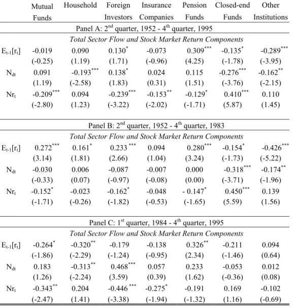
In Table VII, we present the correlation results between flows and the three com-ponents of realized returns given in Equation (23). Panel A reports results using the full sample. Interestingly, the correlations between sector flows and returns for Mu-tual Funds, Foreign Investors and Insurance Companies are seen to be driven mainly by negative correlations betweenflow and news about future expected returns. This correlation is 0.209 for Mutual Funds with a t-statistic of 2.80. For Foreign Investors, the correlation is 0.239 with a t-statistic of 3.22. For Insurance Companies, the cor-relation is 0.153 with a t-statistics of 2.02. Pension fundflows are found to be highly correlated with expected returns.
In Panels B and C, we report correlation results between flows and return compo-nents for the two subsample periods. For the first subperiod, the positive contem-poraneous relations between flows and returns for Mutual funds, Foreign Investors 11Note that in equation (25), news about future expected returns is simply a linear combination
of the innovations to the variables in the VAR equation, where the weight and sign applied to each innovation is based on its coefficient in the market return regression. Since the coefficients on lagged cashflows in the market return regression are negative (see Table IV) these tend to make the relation betweenflows and news about future expected returns more negative.
and Pension Funds are mainly due to flows and the expected component of stock returns. In the second subperiod, the positive correlations for Mutual Funds, For-eign Investors and Insurance Companies are mainly driven by negative correlations betweenflow and news about future expected returns. In addition, the comovements between future return news andflows for these three sectors appear stronger over the second subperiod. For Foreign Investors, there is also a significant relation between flow and news about future dividends.
Based on the results of stock return decomposition, we conclude that the con-temporaneous cashflow-return relations are mainly due to negative relations between flows and news about future expected returns, especially for the second subperiod. This is consistent with the demand shock hypothesis, but does not support the idea that news is being impounded in market prices by the trades of these sectors. We therefore interpret the results of this section as further evidence that these sectors exert pressure on market prices through demand shocks.
VI. CONCLUSION
We find that quarterly stock returns are positively correlated with cashflows from Mutual Funds, Foreign Investors, Pension Funds, and possibly Insurance Companies. To explore the source of these positive correlations, we apply a method of covariance decomposition and find the comovements to be mostly contemporaneous for Mutual Funds, Foreign Investors and Insurance Companies. We then decompose the return shocks into news about future dividends and news about future returns. Sectorflows for Mutual Funds, Foreign Investors and Insurance Companies are found to be neg-atively correlated with news about future returns, while pension fund flows appear to be positively correlated with expected returns. We interpret these findings as ev-idence that Mutual Funds, Foreign Investors and Insurance Companies exert price
with the literature that institutional trades have market impacts.
Evidence that sectorflows affect market prices may have important repercussions on several currentfinancial debates. For instance, such evidence may lead to a greater understanding of the potential impact of investing Social Security money into equity markets, the effect of rapidly growing 401-K plans on stock prices, and the impact of cross-border capital flows onfinancial markets. In addition, the evidence seems to support the popular view that sectorflows by mutual funds drives equity prices.
From a policy perspective, it is especially important to identify the possible market movers and determine the impact of their trading behavior on investor welfare. The results of this paper suggest that the impact of flows on prices does not reflect the dispersion of information to less-informed market participants, but rather, the impact of demand shocks. These insights may be relevant to policy discussions on the merits of imposing capital flow constraints. However, the precise impact of sector flows on investor welfare is not directly studied in this paper and is left for further research.
The dynamics of stock market returns and sector cashflows is extremely intriguing. Further research could explore this relation using time series in higher frequency and possibly identify the source of sector demand shocks.
REFERENCES
[1] Back, K., H. Cao, and G. Wilard, 2000, Imperfect Competition among Informed Traders, Journal of Finance, 55, 2117-2155.
[2] Badrinath, S.G., Jayant R. Kale, and Thomas H. Noe, 1995, Of shepherds, sheep, and the cross-autocorrelations in equity returns, Review of Financial Studies 8, 401-430.
[3] Bekaert, Geert and Robert J. Hodrick, 1992, Characterizing Predictable Components in Excess Returns on Equity and Foreign Exchange Markets, The Journal of Finance 47(2), 467- 410.
[4] Bakshi, Gurdip S. and Zhiwu Chen, 1994, Baby Boom, Population Aging and Capital Markets, Journal of Business, 67, 165-201.
[5] Barclay, M., R. Litzenberger, and J. Warner, 1990, Private Information, Trading Volume, and Stock-return Variances,Review of Financial Studies, 3, 233-253.
[6] Beneish, M.D. and R. Whalley, 1996, An Anatomy of the S&P Game: The Effects of Changing the Rules, Journal of Finance, 1909-1930.
[7] Boyer, Brian H., Tomomi Kumagai, and Kathy Yuan 2002, Are Investors Responsible for Stock Market Contagion?, working paper, University of Michigan.
[8] Cai, Fang, and Lu Zheng, 2000, Institutional Trades and Stock Returns, working paper, University of Michigan.
[9] Chakravarty, S., 2000, Stealth Trading: Which Traders’ Trades Move Stock Prices?, forthcoming, Journal of Financial Economics.
[11] Campbell, John, 1991, A Variance Decomposition for Stock Returns, The Economic Journal 101, 157-179.
[12] Campbell, John and Robert Shiller, 1988a, The Dividend-Price Ratio and Expections of Future Dividends and Discount Factors, Review of Financial Studies 1, 195-228.
[13] Campbell, John and Robert Shiller, 1988b, Stock Prices, Earnings and Expected Dividends, Journal of Finance, 43(3), 661-76.
[14] Campbell, J., S. Grossman and J.Wang, 1993, Trading Volume and Serial Correlation in Stock Returns,The Quarterly Journal of Economics, 108(4), 905-939.
[15] Campbell, John and Albert Kyle, 1993, Smart Money, Noise Trading and Stock Price Behavior, Review of Economic Studies, 60, 1-34.
[16] Chan, Louis and Josef Lakonishok, 1995, The Behavior of Stock Prices Around Insti-tutional Trades,Journal of Finance, 1147-74.
[17] Chan, Louis and Josef Lakonishok, April 1993, Institutional Trades and Intraday Stock Price Behavior, Journal of Financial Economics, 33(2), 173-99.
[18] Chen, Joseph, Harrison Hong and Jeremy Stein, 2000, Breadth of Ownership and Stock Returns, working paper.
[19] Choe, Hyuk, Bong-Chan Kho and Ren´e M. Stulz, 1999, Do foreign investors destablilize stock markets? The Korean experience in 1997,Journal of Financial Economics 54(2), 227-264.
[20] Cohen, R., 1998, Asset Allocation Decisions of Individuals and Institutions, Harvard University, working paper.
[21] Copeland, T. and D. Galai, 1983, Information Effects of the Bid-ask Spread, Journal of Finance, 38, 1457-1469.
[22] Del Guercio, D., 1996, The Distorting Effect of the Prudent-man Laws on Institutional Equity Investment, Journal of Financial Economics, 40, 31-62.
[23] De-Long, J. Bradford, Andrei Shleifer, Lawrence H. Summers and Robert J. Wald-mann, June 1990, Positive Feedback Investment Strategies and Destabilizing Rational Speculation, Journal of Finance, 45(2), 379-395.
[24] Dennis, Patrick J. and Deon Strickland, Who Blinks in Volatile Markets, Individuals or Institutions?, Journal of Finance, forthcoming.
[25] Dornbusch, Rudi and Y.C. Park, 1995, Financial Opening: Policy Lessons for Korea, Korea Institute of Finance, International Center For Economics Growth.
[26] Edelen, Roger, 1999, Investor Flows and the Assessed Performance of Open-end Mu-tual Funds, Journal of Financial Economics 53, 439-466.
[27] Edelen, Roger, and Jerold Warner, 2001, Aggregate Price Effects of Institutional Trading: A Study of Mutual Fund Flow and Market Returns, Journal of Finan-cial Economics 59(2), 195-220.
[28] Elton, Edwin J., Martin J. Gruber, Sanjiv Das, and Mattew Hlavka, 1993, Efficiency with Costly Information: A Reinterpretation of Evidence for Managed Portfolios, Review of Financial Studies 6, 1-22.
[29] Fama, Eugene F., and Kenneth R. French, 1988, Dividend Yields and Expected Stock Returns, Journal of Financial Economics22, 3-25.
[30] Fama, Eugene F., and Kenneth R. French, 1977, Asset Returns and Inflation,Journal of Financial Economics, 5, 115-46.
[31] Ferson, Wayne and Rudi Schadt, 1995, Measuring Fund Strategy and Performance in Changing Economic Conditions, forthcoming, Journal of Finance
[32] Foster, D. and S. Viswanathan, 1996, Strategic Trading when Agents Forecast the Forecasts of Others, Journal of Finance, 51, 1437-1478.
[33] French, K. and R. Roll, 1986, Stock-return Variances: The Arrival of Information and the Reaction of Traders, Journal of Financial Economics17, 5-26.
[34] Froot, K., P. O’Connell and M. Seasholes, 2001, The Portfolio Flow of International Investors, Journal of Financial Economics 59, 151-193.
[35] Glosten, L. and P. Milgrom, 1985, Bid, Ask and Transaction Prices in a Specialist Market with Heterogeneously Informed Traders,Journal of Financial Economics, 14, 71-100.
[36] Griffin, John M., Jeffrey Harris, and Selim Topaloglu, 2001, When do institutions buy and sell? Evidence from the NASDAQ Shakeout, Working Paper, Arizona State University.
[37] Goetzmann, William N. and Massimo Massa, 1998, Index Funds and Stock Market Growth, Yale University Working Paper.
[38] Goetzmann, William and Massimo Massa, 1999, Daily Momentum and Contrarian Behavior of Index Fund Investors, Yale University Working Paper.
[39] Gompers, Paul A., and Andrew Metrick, 2001, Institutional Investors and Equity Prices, Quarterly Journal of Economics 116, 229-259.
[40] Griffin, John M., Jeffrey Harris, and Selim Topaloglu, 2001, When do institutions buy and sell? Evidence from the NASDAQ Shakeout, Journal of Finance, forth-coming.
[41] Grinblatt, M., and S. Titman, and R. Wermers, 1995, Momentum Investment Strate-gies, Portfolio Performance and Herding, A Study of Mutual Fund Behavior, American Economic Review, 85, 1088-1105.
[42] Grossman, S. and M. Miller, 1988, Liquidity and Market Structure, Journal of Fi-nance, 73,617-633.
[43] Gruber, Martin J., 1996, Another Puzzle: the Growth in Actively Managed Mutual Funds, Journal of Finance 51, 783-810.
[44] Hansen, Lars P., 1982, Large Sample Properties of Generalized Method of Moments Estimators, Econometrica 50, 1029-54.
[45] Hong, H. and J. Stein, 1999, A Unified Theory of Underreaction, Momentum Trading, and Overreaction in Asset Markets, Journal of Finance, 54, 2143-2184.
[46] Jones, C., G., Kaul, and M. Lipson, 1994, Transactions, Volume, and Volatility, Review of Financial Studies, 36, 127-154.
[47] Kyle, A., 1985, Continuous Auctions and Insider Trading, Econometrica, 53, 1315-1335.
[48] Lakonishok, Josef, May 1991, Window Dressing by Pension Fund Managers,American Economic Review, 81(2), 227-31.
[49] Lakonishok, Josef, Andrei Shleifer, and Robert W. Vishny, 1991, Do Institutional Investors Destabilize Stock Prices? Evidence on Herding and Feedback Trading, National Bureau of Economic Research Working Paper: 3846.
[50] Newey, Whitney K., and Kenneth D. West, 1987, A Simple Positive Semi-Definite, Heteroskedasticity and Autocorrelation Consistent Covariance Matrix, Econo-metrica, 55, 703-8.