Credit Management Based on Risk Intelligence and its Managerial Implications

(1)

Available at http://www.Jofcis.com

Credit Management Based on Risk Intelligence and

its Managerial Implications

Sung Ho Ha†

School of Business Administration, Kyungpook National University,1370 Daegu, Korea

Abstract

The recent economic crisis not only reduces the profit of retailer stores but also incurs the significant losses caused by increasing the late-payment rate of credit cards. Under this pressure, the scope of credit scoring needs to be broadened to the customer management after delinquency occurs. In doing so, this study clusters the delinquent customers in a department store into homogeneous segments by using a self-organizing map. This study then develops credit prediction models to recognize the repayment patterns of each segment by using a Cox proportional hazard analysis. The credit-scoring models are evaluated and the managerial implications of the study are provided.

Keywords: Credit Management; Risk Intelligence.

1. Introduction

Credit cards of retail stores have some distinct characteristics, when compared with financial credit cards. While the sales of financial credit cards can be generated by the card loans and cash in advance services, the sales generated by the retailer cards mainly come from the merchandise purchases of customers who use them. Retailer credit cards provide such benefits to customers as nearly no interest for purchase, low monthly payments, and purchase financing plans. The principal causes of retailer credit card default have thus come from merchandise sales. Related to this problem, most previous studies have been interested in classifying customer’s credit into two or three groups, such as good/bad customers or good/bad/latent-bad customers, before delinquency occurs. It is difficult to locate research that considers customer groups who can recover from delinquency to normal credit status [1, 2, 3, 4]. Under this circumstance, the credit-scoring research should focus on credit prediction and customer management after delinquency occurs.

Therefore, this study focuses on recoverable customer groups from a credit delinquent state and devises a credit-scoring model for delinquents holding credit cards issued by a department store. This delinquency management employs a hybrid approach to use a self-organizing map (SOM), an artificial neural network, and a Cox’s proportional hazard model, a semi-non-parametric technique for a survival analysis. A SOM is used for clustering credit delinquents into groups with similar characteristics. A Cox’s proportional hazard model is used for predicting the expected time of credit recovery of delinquents by using the influential variables on credit recovery. The hybrid model aims to increasing the efficiency of delinquency risk management of a department store by building differentiated delinquency strategies for each delinquent segment.

†_{Corresponding author.}

(2)

2. Literature Review

Methods used in credit prediction or credit risk assessment are classified into three groups: statistical methods, management scientific methods, and data mining methods [5]. The initial credit-risk management systems used statistical and mathematical programming methods extensively [6][7][8]. Min and Lee [9] proposed a DEA-based approach to credit scoring for the financial data of externally audited 1061 manufacturing firms. Tsaih et al. [10] used a probit regression to develop a credit scoring system for small business loans.

Data mining methods, such as decision trees, neural networks, and genetic algorithms have been used for credit prediction [11][12]. Chen et al. [13] devised an information granulation approach to tackle the class imbalance problem when detecting credit fraud. Abdou et al. [14] investigated neural networks in evaluating a bank’s personal loan data set in Egypt. West [2] investigated five neural network models to credit scoring to find mixture-of-experts and radial basis function neural network models most accurate. Malhotra and Malhotra [15] developed neural networks to classify seven different loan applications of consumers. Hsieh [16] used a SOM neural network to identify profitable groups of customers, based on repayment and recency, frequency, and monetary behavioral scores. West et al. [17] employed a multilayer perceptron neural network with cross-validation, bagging, or boosting strategies for financial decision applications. Huang et al. [18] proposed two-stage genetic programming to improve the accuracy of credit scoring models.

Even though there are many credit prediction models using data mining techniques, it is not easy to tell which one is a winner [4], because data mining techniques cannot guarantee the global optimal solution, owing to over-fitting, or difficulty in building an optimized model [19]. Therefore, it is thought to be more efficient to make the mixed credit prediction models by acquiring the merits from single methods to provide the most optimized solutions [20]. Chen and Huang [1] made up for the weak points of neural networks by using a genetic algorithm. Lee et al. [3] showed the performance of a mixed neural network combined with a discriminant analysis. Zhu et al. [21] implemented a self-organizing learning array system combining with an information theoretic learning capable of solving financial problems. Laha [22] evaluated credit risk by integrating a fuzzy rule based classification and k-nn method.

3. A Hybrid Risk-intelligent Model

This study aims at developing a credit-recovery-predicting model using delinquents’ credit information captured by a typical retail company. As mentioned before, previous researches seldom focused on customers who could recover from a bad credit state to a good credit state. Besides, it is difficult to find research that employs a survival analysis or proportional hazard model in this research purpose. This study devises a hybrid model that combines a SOM and a Cox’s proportional hazard model to improve prediction accuracy. A SOM clusters the credit delinquents into groups with similar characteristics. The resulting clusters of credit delinquents become inputs to a Cox’s hazard model, which is responsible for analyzing patterns of credit recovery from delinquency.

3.1. Neural Clustering of Credit Card Debtors

A clustering analysis is conducted by a SOM with selected variables. To improve the prediction performance, it is important to divide the delinquent customers into several segments with similar characteristics and to compare the repayment patterns among segments. The SOM generates a topological map from input data through a competitive learning process [23]. When an input pattern is imposed on the neural network, the algorithm selects the output node with the smallest Euclidean distance between the presented input pattern vector and its weight vector. Only this winning neuron generates an output signal from the output layer. Because learning involves a weight-vector adjustment, only the neurons in the winning neuron’s neighborhood can learn with this particular input pattern. They do this by adjusting their weights closer to the input vector as follows:

(3)

(

)

( ) ( ) ( )

[

( )

]

( )

, 1 ,

.

j j j j w n n x n w n j N n w n w n otherwise η + − ∈ + =

⎧

_⎨

⎩

(1)

where w_j is a weight vector, x is the presented input vector, η is a learning rate, and N

( )

is a neighborhood function. As learning proceeds, each delinquent within a cluster tends to have similar characteristics, and delinquents in different clusters have different characteristics.

3.2. Statistical Prediction of Repayments

To identify the patterns of credit recovery of delinquent customers, a Cox’s hazard model is chosen because it is useful when an appropriate baseline distribution cannot be identified or when a non-parametric method is necessary. A hazard model statistically analyzes data related to survival time usually in the medical area [24]. A survival analysis uses a likelihood function to build a model that can cover quantitative survival time. Assuming that a survival time t is equal to or greater than zero (t≥0), a probability density function for the survival time t is presented in f t( ), which means a momentary probability that someone can survive at time t but happen to die during Δt. A cumulative density function F t( ) for the time t means that someone has died before or at time t (Equation 2).

(

)

₍

₎

0 0 Pr ( ) lim , ( ) Pr ( ) t t t T t t f t F t T t f u du t Δ → ≤ < + Δ = = ≤ = Δ

∫

(2)

The probability of maintaining a life until time t can be presented as a survival function, S t( ) which can be calculated using the following Equation 3. Therefore, the function f t( ) is calculated by multiplying (-1) by the differential coefficient of the survival function.

(

)

( )

( ) Pr 1 ( ), ( ) dS t

S t T t F t f t

dt

= ≥ = − = − (3) This study recognizes the survival as “delinquency maintenance” and the death as “credit recovery.” When F t( ) explains a cumulative density function of someone who stays in status of good credit to time t, the survival function S t( ) can present the probability of maintaining credit delinquency status until that time. In this case, the density function f t( ) represents the moment of status change, such as from credit delinquency status to credit recovery status. In other words, predicting the credit recovery using the survival analysis is like predicting the death using the survival analysis. The survival rate and the survival function are interpreted as “delinquency maintenance rate” and “delinquency maintenance function.” A hazard function h t( ) calculates the momentary probability of dying at time t, given survival through a certain amount of time t-1. It means that h t( ) can handle the momentary probability of credit recovery at t, assuming that someone has been in a credit delinquency state until t-1. As seen in Equation 4, the hazard rate and hazard function can be used as “credit recovery rate” and “credit recovery function.”

0 Pr( | ) ( ) ( ) lim ( ) t t T t t T t f t h t t S t Δ → ≤ < + Δ ≥ = = Δ (4)

4. Implementation of the Hybrid Risk-intelligent Model

4.1. Segments of Credit Card Debtors

Some credit card customers had late-payment records (41,831) and were found to be valid for clustering of credit card debtors. Five variables were used in clustering: the number of delinquency, the period of delinquency, the amount of delinquency, the time interval between delinquencies, and the number of repayments. To modulate the variances of variables, normalized values were fed into a SOM, which had a 3 by 3 topological map. The detailed training options included that the learning rate = 0.9, the maximum

(4)

number of iterations = 20000, and the convergence criterion = 0.0001. After training the SOM, five segments were derived as seen in Table 1.

Table 1 Clustering Results of the Credit Card Debtors

Segment % of customers Del_times Del_period Del_amount Bet_period Ret_times

DS1 8.92 7.60 1.19 171,310.36 1.50 1.04

DS2 35.0 3.06 1.39 140,062.98 3.45 1.13

DS3 18.57 1.43 4.76 168,045.54 0.48 3.25

DS4 37.16 1.09 1.08 114,572.35 0.09 1.00

DS5 0.34 2.21 1.81 2,807,052.06 1.19 1.48

Debtor Segment 1 (DS1) contains the most frequent debtors with the highest number of delinquency (around eight times), who immediately repay in full once being recorded as delinquents. These customers seem to become credit delinquents because of the difference between the monthly closing date and the actual repayment date. Debtor Segment 2 (DS2) contains all the 14,641 delinquents who have such characteristics as the average number of repayments = 1, the overdue amount = 140,000, and the frequency of delinquency = 3. Segments DS1 and DS2 do not have a lot of late payments but have a high number of overdue, and therefore, customers in these segments are thought to be habitual delinquents.

Debtor Segment 3 (DS3) contains 7,769 delinquents. The characteristics of this group are summarized as follows: the average number of repayments = more than 3 times, the delinquent period = 5 months, the overdue amount = 160,000, and the number of delinquency = below 2 times. Customers in this segment have the longest delinquency period and repay small amounts of money relatively often. Debtor Segment 4 (DS4) is the largest and customers in this segment seem to repay their delinquent amount at once. Debtor Segment 5 (DS5) has a relatively large delinquent amount (3 million, on average) and repays it by an average of 1.5 installments for two months. In spite of a small portion of delinquents (143), the average amount of delinquency is almost 20 times larger than other segments.

4.2. Repayment Patterns of each Segment

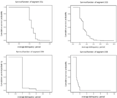
To analyze the patterns of credit recovery, 16,099 delinquents were randomly sampled from the segmented delinquents. A set of 18 variables was arranged to build hazard models: five variables used in clustering and 13 new variables including demographic and purchasing transaction information. Fig. 1 illustrates the resulting graphs of survival functions for each segment.

In this study, “Cox Regression Model of Survival Analysis” in SPSS was used to build the hazard models to analyze the patterns of credit recovery for each segment. The total time period of delinquency was entered as a time variable and the status variable had a value of one for credit recovery and zero for credit delinquency. Other variables were selected as input variables. “Stepwise forward” was chosen as a variable input method and “Likelihood-ratio statistics based on the conditional parameter estimate” was chosen as a variable removal method. The significance level of this model was set to 0.005. Table 2 shows the cumulative hazard function of each segment, which was generated by the hazard models.

5. Validation of the Hybrid Risk-intelligent Model

5.1. Experiments for each Segment and Comparison with other Techniques

Those models deploying C5.0, Support Vector Machine (SVM), and Neural Network (NN) techniques were developed for making comparisons with the Cox survival analysis. Given the debtor segments produced by the SOM, for all models the same training data set and validation data set were used. First of all, C5.0 adopted a boosting method and a local/global pruning in training. A branch of the tree was split

(5)

only if the sub-branches contained at least two records. The actual credit recovery month was the target response variable and entropy was the impurity measurement.

Fig. 1 The Survival Functions of the Segments

Table 2 Hazard Models for Segments, DS1, DS2, DS3, DS4, and DS5

Segment Hazard model

DS1

1( ) 0 exp(0.205 _ _ 0.605 _

3.738 _ 0.006 0.102 )

( )

H t H PUR YM CNT BET PERIOD

RET TIMES AGE MARRIAGE

t = − − − + × × × × × × 1( ) exp[ 1( )] S t = −H t DS2 2( ) 0 exp(0.1 _ _ 0.045 _ 0.051 _ 1.419 _ ) ( )

H t H PUR YM CNT DEL TIMES

BET PERIOD RET TIMES

t = − − − × × × × × 2( ) exp[ 2( )] S t = −H t DS3 3( ) 0 exp(0.12 _ _ 0.007 _ _ 0.097 _ 0.310 _ 0.01 0.018 _ _ 0.019 ( )

H t H PUR YM CNT PUR YMD CNT

DEL TIMES RET TIMES

AGE MEM REG PERIOD

C t = − + − + + − × × × × × × ×

× ARD_ISSUE_PERIOD)

3( ) exp[ 3( )] S t = −H t DS4 4 0 ( ) ( ) exp(0.015 _ _ ) H t =H t × ×PUR YM CNT 4( ) exp[ 4( )] S t = −H t DS5 5 0 ( ) ( ) exp( 2.005 _ ) H t =H t × − ×RET TIMES 5( ) exp[ 5( )] S t = −H t

SVM adopted a radial basis function as the kernel function and set the regularization parameter = 10, the regression precision = 0.1 and the RBF gamma = 0.1. NN placed 19 neurons in the first hidden layer, 5 neurons in the second hidden layer, and 11 neurons in the output layer. NN set the learning rate to 0.9 and the momentum to 0.3, which were decaying gradually to 0.01. Fig. 2 shows the gain charts for the four models being compared on the validation set. The gain charts illustrate, for each decile, the percentage of

(6)

predicted events (here, credit recovery). The larger the area between the gain chart and the diagonal line, the better the considered model. It appears that the gain charts for all four models are rather similar and they have a similar performance.

To decide between the curves, more information is needed about the prediction performance. This study measured the prediction accuracy rates for the models: all were calculated after performing 20-time experiments using the different random partitioning of the data. On the validation set, the Cox model proved to be the best, followed by the NN model, the SVM model, and then the C5.0 model. However, the differences were rather slight, as shown in Table 3.

Fig. 2 Gain Charts for the Models, Applied to the Validation Data Table 3 Prediction Accuracy Rates for each Model

Cox C5.0 SVM NN

Average 0.9326 0.8891 0.8940 0.8993

Variance 0.00001 0.00004 0.00004 0.00004

It turned out that the NN model won the first place for the segments DS1 and DS3, and the Cox model outperformed the other models for the segments DS2, DS4, and DS5. Table 4 shows the confusion matrices for the Cox model with the customer segments. The segments DS1, DS2, DS4, and DS5 led to a higher type II error. The segment DS3, however, resulted in a higher type I error. In addition, the segment DS3 had the highest type I error probability among all the considered models. Notice that those segments with a shorter delinquent period scored good prediction accuracy: 1.1 for segment DS4, 1.2 for segment DS1, 1.4 for segment DS2, 1.7 for segment DS5, and 3.5 for segment DS3.

Table 4 Confusion Matrices for the Cox Model

Predicted Segment Delinquent Non-delinquent DS1 Observed Delinquent 0.4830 0.0067 Non-delinquent 0.0000 0.5103 DS2 Observed Delinquent 0.4916 0.0436 Non-delinquent 0.0008 0.4640 DS3 Observed Delinquent 0.7517 0.0436 Non-delinquent 0.1557 0.0490 DS4 Observed Delinquent 0.4844 0.0248 Non-delinquent 0.0000 0.4908 DS5 Observed Delinquent 0.6473 0.0290 Non-delinquent 0.0000 0.3237

(7)

5.2. Implications for Credit Management

The focal company gets earnings from credit-recovering customers. In this section, the expected earnings from credit recovery were calculated by using the developed credit-scoring models. Table 5 summarizes the expected number of credit recovery by each segment on a monthly basis. The validation data set (5365 customers) was used in the calculation of expected earnings.

Table 5 Expected Number of Credit Recovery on a Monthly Basis Expected Number of Credit Recovery

DS1 DS2 DS3 DS4 DS5 Total % 1st_month_{0 0 0 0 1 1}_0.01 2nd_month₆₂₀_{1460 0 1889 18 3987}_74.32 3rd_month_{0 637 2 0 2 641}_11.94 4th_month ₀ ₁₂₄ ₁₅ ₀ ₁ ₁₄₀ _2.60 5th_month_{0 25 61 0 0 86}_1.60 6th_month_{0 42 190 0 0 232}_4.32 7th_month_{0 0 95 0 1 96}_1.78 8thmonth 0 0 70 0 0 70 1.30 9thmonth 0 0 43 0 0 43 0.80 10th_month_{0 0 36 0 0 36}_0.67 11th_month_{0 0 17 0 0 17}_0.31 12th_month_{0 0 16 0 0 16}_0.29

According to Table 5, every segment (except segment DS3) had the highest number of credit recovery at the 2nd month (74.32%), followed by the 3rd month (11.94%). The expected earnings from each credit-recovering customer can be calculated by adding the amount of repayment at the predicted recovery month to the late fees until credit recovery (Equation 5). The late fee can be calculated from the formula, p * (delinquency amount * r), where p means the period of delinquency and r indicates the interest rate.

The expected amount of revenue per delinquent = late fee + repayment amount (5) Table 6 summarizes the total amount of revenue predicted for each segment. Most revenue is predicted to be earned from segment DS2 (38.57%), followed by DS4 (28.39%). From the perspective of delinquency risk management, several managerial clues are found from these tables. The credit management department needs to focus on the predicted revenue incurred at the 2nd month, at which most customers in segments DS1, DS2, DS4, and DS5 have recovered from delinquency. Moreover, sending simple emails or messages that remind customers in segments DS1, DS2, and DS4 of the settlement date is much helpful, because these people habitually delay the payment of credit card bills. Delinquency could be thought as a misunderstanding of the settlement date. Therefore, encouragement of using an automatic settlement system is another method to prevent this kind of delinquency in advance. For segment DS3, the credit management department needs to lower the credit rating to the extent customers in the segment can pay the full costs.

Table 6 Amount of Revenue Predicted by each Segment (r = 10%) Segment Late Fee Amount of

Repayment Total Revenue %

DS1 12,999,961 109,243,371 122,243,332 12.53 DS2 46,184,493 329,889,234 376,073,727 38.57 DS3 43,865,189 90,630,556 134,495,745 13.79 DS4 26,984,112 249,852,891 276,837,003 28.39 DS5 10,033,196 55,432,024 65,465,220 6.71 Total 140,066,952 835,048,076 975,115,028 100.00 6. Conclusion

This study presented a credit-scoring method to solve common problems of credit card debt in a typical retail store. The contributions of this study are summarized as follows. First, while most previous research on credit scoring has focused on classifying customers into two groups of good/bad credit customers, this study made it possible to analyze the delinquent customers who had recovered from a credit delinquency

(8)

state to a good credit state. Second, this study used a survival analysis to identify the influential variables on the rate of credit recovery and to predict the time of credit recovery. Third, this study calculates the expected earnings after credit recovery and demonstrates several managerial clues to deal with delinquency risk. This study, however, has some limitations that are improved in future research. First, it used only 12 months of data associated with the credit delinquents of a single department store. This made it difficult to generalize the research results. Therefore, various types of variables for multiple periods need to be collected and analyzed for generalization of this type of research. Second, this study focused on those delinquents who had recovered from a credit delinquency state, but a future study needs to encompass all kinds of customers from good to bad credit in order to develop a more complete credit-scoring system.

References

[1] M.C. Chen and S.H. Huang. Credit scoring and rejected instances reassigning through evolutionary computation techniques. Expert Systems with Applications, 2003, 24(4): 433-441.

[2] D. West. Neural network credit scoring models. Computers and Operations Research, 2000, 27(11-12): 1131-1152.

[3] T.S. Lee, C.C. Chiu, C.J. Lu, and I.F. Chen. Credit scoring using the hybrid neural discriminant technique. Expert Systems with Applications, 2002, 23(3): 245-254.

[4] L.C. Thomas. A survey of credit and behavioral scoring: Forecasting financial risk of lending to consumers. International Journal of Forecasting, 2000, 16(2): 149-172.

[5] J.N. Crook, D.B. Edelman, and L.C. Thomas. Recent developments in consumer credit risk assessment. European Journal of Operational Research, 2007, 183(3): 1447-1465.

[6] D.R. Cox. Regression models and life-tables. Journal of the Royal Statistical Society, 1972, 34(2): 187-220. [7] P.S. Bradley, U.M. Fayyad, and O.L. Mangasarian. Mathematical programming for data mining: formulations

and challenges. INFORMS Journal on Computing, 1999, 11(3): 217-238.

[8] S.H. Ha and E.K. Kwon. Business intelligence for delinquency risk management via Cox regression. Lecture Notes in Artificial Intelligence, 2010, 6232: 82-90.

[9] J.H. Min, Y.-C. Lee. A practical approach to credit scoring. Expert Systems with Applications, 2008, 35(4): 1762-1770.

[10] R. Tsaih, Y.-J. Liu, W. Liu, and Y.-L. Lien. Credit scoring system for small business loans. Decision Support Systems, 2004, 38(1): 91-99.

[11] X. Hu. A data mining approach for retailing bank customer attrition analysis. Applied Intelligence, 2005, 22(1): 47-60.

[12] M.J.A. Berry and G. Linoff. Data Mining Techniques (Second eds.). Wiley, Indianapolis (2004).

[13] M.-C. Chen, L.-S. Chen, C.-C. Hsu, and W.-R. Zeng. An information granulation based data mining approach for classifying imbalanced data. Information Sciences, 2008, 178(16): 3214-3227.

[14] H. Abdou, J. Pointon, and A. El-Masry. Neural nets versus conventional techniques in credit scoring in Egyptian banking. Expert Systems with Applications, 2008, 35(3): 1275-1292.

[15] R. Malhotra, D.K. Malhotra. Evaluating consumer loans using neural networks. Omega, 2003, 31(2): 83-96. [16] N.-C. Hsieh. An integrated data mining and behavioral scoring model for analyzing bank customers. Expert

Systems with Applications, 2004, 27(4): 623-633.

[17] D. West, S. Dellana, and J. Qian. Neural network ensemble strategies for financial decision applications. Computers and Operations Research, 2005, 32(10): 2543-2559.

[18] J.-J. Huang, G.-H. Tzeng, and C.-S. Ong. Two-stage genetic programming (2SGP) for the credit scoring model. Applied Mathematics and Computation, 2006, 174(2): 1039-1053.

[19] J.V. Hansen. Combining predictors: comparison of five meta machine learning methods. Information Sciences, 1999, 119(1-2): 91-105.

[20] W. Chen, C. Ma, and L. Ma. Mining the customer credit using hybrid support vector machine technique. Expert Systems with Applications, 2009, 36(4): 7611-7616.

[21] Z. Zhu, H. He, J.A. Starzyk, and C. Tseng. Self-organizing learning array and its application to economic and financial problems. Information Sciences, 2007, 177(5): 1180-1192.

[22] A. Laha. Building contextual classifiers by integrating fuzzy rule based classification technique and k-nn method for credit scoring. Advanced Engineering Informatics, 2007, 21(3): 281-291.

(9)

[23] T. Kohonen. Self-Organizing Maps (Third eds.). Springer-Verlag, Berlin (2001).

[24] L.N. Allen, and L.C. Rose. Financial survival analysis of defaulted debtors. Journal of the Operational Research Society, 2006, 57(6): 630-636.