Journal of Statistical Software
February 2020, Volume 92, Issue 10. doi: 10.18637/jss.v092.i10
bridgesampling: An
R
Package for Estimating
Normalizing Constants
Quentin F. Gronau University of Amsterdam Henrik Singmann University of Warwick Eric-Jan Wagenmakers University of Amsterdam AbstractStatistical procedures such as Bayes factor model selection and Bayesian model averag-ing require the computation of normalizaverag-ing constants (e.g., marginal likelihoods). These normalizing constants are notoriously difficult to obtain, as they usually involve high-dimensional integrals that cannot be solved analytically. Here we introduce anRpackage that uses bridge sampling (Meng and Wong 1996; Meng and Schilling 2002) to estimate normalizing constants in a generic and easy-to-use fashion. For models implemented in Stan, the estimation procedure is automatic. We illustrate the functionality of the package with three examples.
Keywords: bridge sampling, marginal likelihood, model selection, Bayes factor, Warp-III.
1. Introduction
In many statistical applications, it is essential to obtain normalizing constants of the form Z =
Z
Θ
q(θ) dθ, (1)
where p(θ) = q(θ)/Z denotes a probability density function (pdf) defined on the domain
Θ ⊆ Rp. For instance, the estimation of normalizing constants plays a crucial role in free
energy estimation in physics, missing data analyses in likelihood-based approaches, Bayes factor model comparisons, and Bayesian model averaging (e.g., Gelman and Meng 1998). In this article, we focus on the role of the normalizing constant in Bayesian inference; however, the bridgesamplingpackage (Gronau and Singmann 2020) can be used in any context where one desires to estimate a normalizing constant.
In Bayesian inference, the normalizing constant of the joint posterior distribution is involved in (a) parameter estimation, where the normalizing constant ensures that the posterior integrates
to one; (b) Bayes factor model comparison, where the ratio of normalizing constants quantifies the data-induced change in beliefs concerning the relative plausibility of two competing models (e.g.,Kass and Raftery 1995); (c) Bayesian model averaging, where the normalizing constant is required to obtain posterior model probabilities (BMA; Hoeting, Madigan, Raftery, and Volinsky 1999).
For Bayesian parameter estimation, the need to compute the normalizing constant can usu-ally be circumvented by the use of sampling approaches such as Markov chain Monte Carlo (MCMC; e.g.,Gamerman and Lopes 2006). However, for Bayes factor model comparison and BMA, the normalizing constant of the joint posterior distribution – in this context usually called marginal likelihood – remains of essential importance. This is evident from the fact that the posterior model probability of modelMi, i∈ {1,2, . . . , m},given datayis obtained
as
p(Mi|y)
| {z }
posterior model probability
= p(y| Mi) Pm j=1p(y| Mj)p(Mj) | {z } updating factor × p(Mi) | {z }
prior model probability
, (2)
where p(y| Mi) denotes themarginal likelihood of modelMi.
If the model comparison involves only two models,M1 and M2, it is convenient to consider the odds of one model over the other. Bayes’ rule yields:
p(M1 |y) p(M2 |y) | {z } posterior odds = p(y| M1) p(y| M2) | {z } Bayes factor BF12 × p(M1) p(M2) | {z } prior odds . (3)
The change in odds brought about by the data is given by the ratio of the marginal likelihoods of the models and is known as the Bayes factor (Jeffreys 1961; Kass and Raftery 1995;Etz and Wagenmakers 2017). Equations 2 and 3 highlight that the normalizing constant of the joint posterior distribution, that is, the marginal likelihood, is required for computing both posterior model probabilities and Bayes factors.
The marginal likelihood is obtained by integrating out the model parameters with respect to their prior distribution:
p(y| Mi) =
Z
Θ
p(y|θ,Mi)p(θ| Mi) dθ. (4) The marginal likelihood implements the principle of parsimony also known asOccam’s razor (e.g., Jefferys and Berger 1992;Myung and Pitt 1997;Vandekerckhove, Matzke, and Wagen-makers 2015). Unfortunately, the marginal likelihood can be computed analytically for only a limited number of models. For more complicated models (e.g., hierarchical models), the marginal likelihood is a high-dimensional integral that usually cannot be solved analytically. This computational hurdle has complicated the application of Bayesian model comparisons for decades.
To overcome this hurdle, a range of different methods have been developed that vary in ac-curacy, speed, and complexity of implementation: naive Monte Carlo estimation, importance sampling, the generalized harmonic mean estimator, reversible jump MCMC (Green 1995), the product-space method (Carlin and Chib 1995;Lodewyckx, Kim, Lee, Tuerlinckx, Kup-pens, and Wagenmakers 2011), Chib’s method (Chib 1995), thermodynamic integration (e.g., Lartillot and Philippe 2006), path sampling (Gelman and Meng 1998), and others. The ideal
method is fast, accurate, easy to implement, general, and unsupervised, allowing non-expert users to treat it as a “black box”.
In our experience, one of the most promising methods for estimating normalizing constants is bridge sampling (Meng and Wong 1996;Meng and Schilling 2002). Bridge sampling is a general procedure that performs accurately even in high-dimensional parameter spaces such as those that are regularly encountered in hierarchical models. In fact, simpler estimators such as the naive Monte Carlo estimator, the generalized harmonic mean estimator, and importance sampling are special sub-optimal cases of the bridge identity described in more detail below (e.g.,Frühwirth-Schnatter 2004;Gronauet al. 2017).
In this article, we introducebridgesampling, an R(RCore Team 2019) package that enables the straightforward and user-friendly estimation of the marginal likelihood (and of normal-izing constants more generally) via bridge sampling techniques and which is available from the ComprehensiveRArchive Network (CRAN) athttps://CRAN.R-project.org/package= bridgesampling. In general, the user needs to provide to thebridge_sampler function four
quantities that are readily available:
• an object with posterior samples (argument samples);
• a function that computes the log of the unnormalized posterior density for a set of model parameters (argument log_posterior);
• a data object that contains the data and potentially other relevant quantities for eval-uating log_posterior(argument data);
• lower and upper bounds for the parameters (arguments lband ub, respectively).
Given these inputs, the bridgesampling package provides an estimate of the log marginal likelihood.
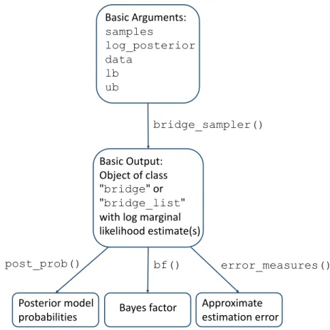
Figure 1 displays the steps that a user may take when using the bridgesampling package. Starting from the top, the user provides the basic required arguments to thebridge_sampler
function which then produces an estimate of the log marginal likelihood. With this estimate in hand – usually for at least two different models – the user can compute posterior model probabilities using the post_prob function, Bayes factors using the bf function, and
ap-proximate estimation errors using the error_measures function. A schematic call of the bridge_sampler function looks as follows (detailed examples are provided in the next
sec-tions):
bridge_sampler(samples = samples, log_posterior = log_posterior, data = data, lb = lb, ub = ub)
Thebridge_samplerfunction is aS3 generic which currently has methods for objects of class
‘mcmc’, ‘mcmc.list’ (Plummer, Best, Cowles, and Vines 2006), ‘stanfit’ (StanDevelopment Team 2016a), ‘matrix’, ‘rjags’ (Plummer 2016; Su and Yajima 2015), ‘runjags’ (Denwood
2016), ‘stanreg’ (StanDevelopment Team 2016b), and for ‘MCMC_refClass’ objects produced
by nimble (de Valpine, Turek, Paciorek, Anderson-Bergman, Lang, and Bodik 2017).1 This 1
We thank Ben Goodrich for adding the ‘stanreg’ method to our package and Perry de Valpine for his help implementing thenimblesupport.
Basic Arguments: samples log_posterior data lb ub bridge_sampler() Basic Output: Object of class "bridge" or "bridge_list" with log marginal likelihood estimate(s) bf() post_prob() error_measures() Approximate estimation error Bayes factor Posterior model probabilities
Figure 1: Flow chart of the steps that a user may take when using thebridgesamplingpackage. In general, the user needs to provide a posterior samples object (samples), a function that
computes the log of the unnormalized posterior density (log_posterior), the data (data),
and parameter bounds (lbandub). Thebridge_samplerfunction then produces an estimate
of the log marginal likelihood. This is usually repeated for at least two different models. The user can then compute posterior model probabilities (using the post_prob function), Bayes
factors (using thebffunction), and approximate estimation errors (using theerror_measures
function). Note that the summary method for bridge objects automatically invokes the
error_measures function. Figure also available athttps://tinyurl.com/ybf4jxka. allows the user to obtain posterior samples in a convenient and efficient way, for instance, via JAGS (Plummer 2003) or a highly customized sampler. Hence, bridge sampling does
not require users to program their own MCMC routines to obtain posterior samples; this convenience is usually missing for methods such as reversible jump MCMC (but see Gelling, Schofield, and Barker 2017).
When the model is specified in Stan (Carpenter et al.2017;Stan Development Team 2016a) – in a way that retains the constants, as described below – obtaining the marginal likelihood is even simpler: the user only needs to pass the ‘stanfit’ object to the bridge_sampler
function. The combination of Stan and the bridgesampling package therefore produces an unsupervised, black box computation of the marginal likelihood.
This article is structured as follows: First we describe the implementation details of the algorithm from bridgesampling; second, we illustrate the functionality of the package using a
simple Bayesiant-test example where posterior samples are obtained viaJAGS. In this section,
we also explain a heuristic to obtain the function that computes the log of the unnormalized posterior density inJAGS; third, we describe in more detail the interface toStanwhich enables
an even more automatized computation of the marginal likelihood. Fourth, we illustrate use of theStaninterface with two well-known examples from the Bayesian model selection literature.
2. Bridge sampling: The algorithm
Bridge sampling can be thought of as a generalization of simpler methods for estimating nor-malizing constants such as the naive Monte Carlo estimator, the generalized harmonic mean estimator, and importance sampling (e.g., Frühwirth-Schnatter 2004; Gronau et al. 2017).
These simpler methods typically use samples from a single distribution, whereas bridge sam-pling combines samples from two distributions.2 For instance, in its original formulation (Meng and Wong 1996), bridge sampling was used to estimate a ratio of two normalizing con-stants such as the Bayes factor. In this scenario, the two distributions for the bridge sampler are the posteriors for each of the two models involved. However, the accuracy of the estimator depends crucially on the overlap between the two involved distributions; consequently, the accuracy can be increased by estimating a single normalizing constant at a time, using as a second distribution a convenient normalized proposal distribution that closely matches the distribution of interest (e.g., Gronau et al. 2017; Overstall and Forster 2010). The bridge
sampling estimator of the marginal likelihood is then given by:3 p(y) = Eg(θ)[h(θ)p(y|θ)p(θ)] Ep(θ|y)[h(θ)g(θ)] ≈ 1 n2 Pn2 j=1h( ˜θj)p(y|θ˜j)p( ˜θj) 1 n1 Pn1 i=1h(θi∗)g(θi∗) , (5)
where h(θ) is called the bridge function and g(θ) denotes the proposal distribu-tion. {θ1∗,θ∗2, . . . ,θn∗1} denote n1 samples from the posterior distribution p(θ|y) and
{θ1,˜ θ2˜ , . . . ,θ˜n2}denote n2 samples from the proposal distributiong(θ).
To use bridge sampling in practice, one has to specify the bridge functionh(θ) and the pro-posal distributiong(θ). For the bridge functionh(θ), thebridgesamplingpackage implements the optimal choice presented in Meng and Wong (1996) which minimizes the relative mean-squared error of the estimator. Using this particular bridge function, the bridge sampling estimate of the marginal likelihood is obtained via an iterative scheme that updates an initial guess of the marginal likelihood ˆp(y)(0) until convergence (for details, see Meng and Wong 1996;Gronauet al. 2017). The estimate at iteration t+ 1 is obtained as follows:
ˆ p(y)(t+1)= 1 n2 n2 P j=1 l2,j s1l2,j+s2pˆ(y)(t) 1 n1 n1 P i=1 1 s1l1,i+s2pˆ(y)(t) , (6) wherel1,i= p(y |θ∗i)p(θ∗i) g(θi∗) , andl2,j= p(y|θ˜j)p( ˜θj)
g( ˜θj) . In practice, a more numerically stable version
of Equation 6 is implemented that uses logarithms in combination with the Brobdingnag
2
Note, however, that these simpler methods are special cases of bridge sampling (e.g.,Gronauet al.2017, Appendix A). Hence, for particular choices of the bridge function and the proposal distribution, only samples from one distribution are used.
3
We omit conditioning on the model for enhanced legibility. It should be kept in mind, however, that this yields the estimate of the marginal likelihood for a particular modelMi, that is,p(y| Mi).
R package (Hankin 2007) to avoid numerical under- and overflow (for details, see Gronau
et al.2017, Appendix B).
The iterative scheme usually converges within a few iterations. Note that, crucially,l1,i and
l2,j need only be computed once before the iterative updating scheme is started. In practice,
evaluating l1,i and l2,j takes up most of the computational time. Luckily, l1,i and l2,j can
be computed completely in parallel for each i ∈ {1,2, . . . , n1} and each j ∈ {1,2, . . . , n2},
respectively. That is, in contrast to MCMC procedures, the evaluation of, for instance, l1,i+1 does not require one to evaluate l1,i first (since the posterior samples and proposal
samples are already available). The bridgesampling package enables the user to compute l1,i and l2,j in parallel by setting the argument cores to an integer larger than one. On
Unix/macOS machines, this parallelization is implemented using the parallel package. On Windows machines this is achieved using the snowfall package (Knaus 2015).4
After having specified the bridge function, one needs to choose the proposal distributiong(θ). The bridgesampling package implements two different choices: (a) a multivariate normal proposal distribution with mean vector and covariance matrix that match the respective posterior samples quantities and (b) a standard multivariate normal distribution combined with a warped posterior distribution.5 Both choices increase the efficiency of the estimator by making the proposal and the posterior distribution as similar as possible. Note that under the optimal bridge function, the bridge sampling estimator is robust to the relative tail behavior of the posterior and the proposal distribution. This stands in sharp contrast to the importance and the generalized harmonic mean estimator for which unwanted tail behavior produces estimators with very large or even infinite variances (e.g., Owen and Zhou 2000; Frühwirth-Schnatter 2004;Gronauet al. 2017).
2.1. Option I: The multivariate normal proposal distribution
The first choice for the proposal distribution that is implemented in thebridgesampling pack-age is a multivariate normal distribution with mean vector and covariance matrix that match the respective posterior samples quantities. This choice (henceforth “the normal method”) generalizes to high dimensions and accounts for potential correlations in the joint poste-rior distribution. This proposal distribution is obtained by setting the argument method = "normal" in the bridge_sampler function; this is the default setting. This choice assumes
that all parameters are allowed to range across the entire real line. In practice, this assump-tion may not be fulfilled for all components of the parameter vector, however, it is usually possible to transform the parameters so that this requirement is met. This is achieved by transforming the original p-dimensional parameter vector θ (which may contain components that range only across a subset ofR) to a new parameter vectorξ (where all components are
allowed to range across the entire real line) using a diffeomorphic vector-valued functionf so that ξ =f(θ). By the change-of-variable rule, the posterior density with respect to the new parameter vector ξ is given by:
p(ξ |y) =pθ(f−1(ξ)|y) det h Jf−1(ξ) i , (7) 4
Due to technical limitations specific to Windows, this parallelization is not available for the ‘stanfit’ and ‘stanreg’ methods.
5
Note that other proposal distributions such as multivariatetdistributions are conceivable but are currently not implemented in thebridgesamplingpackage.
wherepθ(f−1(ξ)|y) refers to the untransformed posterior density with respect toθevaluated
forf−1(ξ) = θ. Jf−1(ξ) denotes the Jacobian matrix with the element in the i-th row and
j-th column given by ∂θi
∂ξj. Crucially, the posterior density with respect to ξ retains the
normalizing constant of the posterior density with respect to θ; hence, one can select a convenient transformation without changing the normalizing constant. Note that in order to apply a transformation no new samples are required; instead the original samples can simply be transformed using the function f.
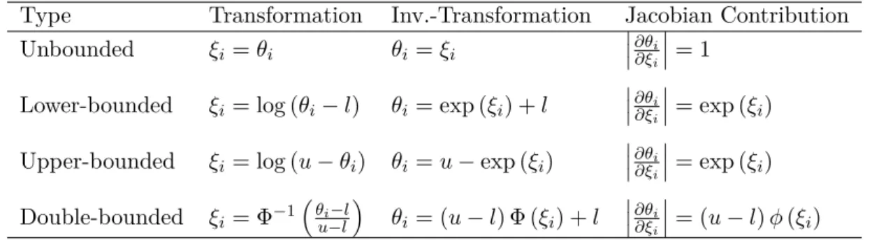
In principle, users can select transformations themselves. Nevertheless, the bridgesampling package comes with a set of built-in transformations (see Table 2.1), allowing the user to work with the model in a familiar parameterization. When the user then supplies a named vector with lower and upper bounds for the parameters (argumentslb andub, respectively),
the package internally transforms the relevant parameters and adjusts the expressions by the Jacobian term. Furthermore, as will be elaborated upon below, when the model is fitted in
Stan, thebridgesamplingpackage takes advantage of the rich class of Stan transformations.
The transformations built into the bridgesampling package are useful whenever each com-ponent of the parameter vector can be transformed separately.6 In this scenario, there are four possible cases per parameter: (a) the parameter is unbounded; (b) the parameter has a lower bound (e.g., variance parameters); (c) the parameter has an upper bound; and (d) the parameter has a lower and an upper bound (e.g., probability parameters). As shown in Table2.1, in case (a) the identity (i.e., no) transformation is applied. In case (b) and (c), log-arithmic transformations are applied to transform the parameter to the real line. In case (d) a probit transformation is applied. Note that internally, the posterior density is automatically adjusted by the relevant Jacobian term. Since each component is transformed separately, the resulting Jacobian matrix will be diagonal. This is convenient since it implies that the absolute value of the determinant is the product of the absolute values of the diagonal entries of the Jacobian matrix:
det h Jf−1(ξ) i = p Y i=1 ∂θi ∂ξi . (8)
Once all posterior samples have been transformed to the real line, a multivariate normal distribution is fitted using method-of-moments. On a side note, bridge sampling may under-estimate the marginal likelihood when the same posterior samples are used both for fitting the proposal distribution and for the iterative updating scheme (i.e., Equation 6). Hence, as recommended by Overstall and Forster (2010), the bridgesampling package divides each MCMC chain into two halves, using the first half for fitting the proposal distribution and the second half for the iterative updating scheme.
2.2. Option II: Warping the posterior distribution
The second choice for the proposal distribution that is implemented in the bridgesampling package is a standard multivariate normal distribution in combination with awarpedposterior distribution. The goal is still to match the posterior and the proposal distribution as closely as possible. However, instead of manipulating the proposal distribution, it is fixed to a
6Thanks to a recent pull request by Kees Mulder, the bridgesamplingpackage now also supports a more complicated case in which multiple parameters are constrained jointly (i.e., simplex parameters). This pull request also added support for circular parameters.
Type Transformation Inv.-Transformation Jacobian Contribution Unbounded ξi=θi θi =ξi ∂θi ∂ξi = 1
Lower-bounded ξi= log (θi−l) θi = exp (ξi) +l
∂θi ∂ξi = exp (ξi)
Upper-bounded ξi= log (u−θi) θi =u−exp (ξi)
∂θi ∂ξi = exp (ξi) Double-bounded ξi= Φ−1 θ i−l u−l θi = (u−l) Φ (ξi) +l ∂θi ∂ξi = (u−l)φ(ξi)
Table 1: Overview of built-in transformations in thebridgesamplingpackage. ldenotes a pa-rameter lower bound andudenotes an upper bound. Φ(·) denotes the cumulative distribution
function (cdf) and φ(·) the probability density function (pdf) of the normal distribution.
standard multivariate normal distribution, and the posterior distribution is manipulated (i.e., warped). Crucially, the warped posterior density retains the normalizing constant of the original posterior density. The general methodology is referred to as Warp bridge sampling (Meng and Schilling 2002).
There exist several variants of Warp bridge sampling; in the bridgesampling package, we implemented Warp-III bridge sampling (Meng and Schilling 2002; Overstall 2010; Gronau, Wagenmakers, Heck, and Matzke 2019) which can be used by setting method = "warp3".
This version matches the first three moments of the posterior and the proposal distribution. That is, in contrast to the simpler normal method described above, Warp-III not only matches the mean vector and the covariance matrix of the two distributions, but also the skewness. Consequently, when the posterior distribution is skewed, Warp-III may result in an estimator that is less variable. When the posterior distribution is symmetric, both Warp-III and the normal method should yield estimators that are about equally efficient. Hence, in principle, Warp-III should always provide estimates that are at least as precise as the normal method. However, the Warp-III method also takes about twice as much time to execute as the normal method; the reason for this is that Warp-III sampling results in a mixture density (for details, seeOverstall 2010;Gronauet al.2019) which requires that the unnormalized posterior density
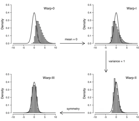
is evaluated twice as often as in the normal method. Figure2 illustrates the intuition for the warping procedure in the univariate case. The gray histogram in the top-left panel depicts skewed posterior samples, the solid black line the standard normal proposal distribution. The Warp-III procedure effectively standardizes the posterior samples so that they have mean zero (top-right panel) and variance one (bottom-right panel), and then attaches a minus sign with probability 0.5 to the samples which achieves symmetry (bottom-left panel). This intuition naturally generalizes to the multivariate case. Starting with posterior samples that can range across the entire real line (i.e., ξ) the multivariate Warp-III procedure is based on the following stochastic transformation:
η= b |{z} symmetry × R−1 | {z } covarianceI × (ξ−µ) | {z } mean 0 , (9)
where b ∼ B(0.5) on {−1,1} and µ corresponds to the expected value of ξ (i.e., the mean vector).7 The matrixR is obtained via the Cholesky decomposition of the covariance matrix
Warp-0 -10 -5 0 5 10 0.0 0.1 0.2 0.3 0.4 0.5 Density mean = 0 Warp-I -10 -5 0 5 10 0.0 0.1 0.2 0.3 0.4 0.5 Density variance = 1 Warp-II -10 -5 0 5 10 0.0 0.1 0.2 0.3 0.4 0.5 Density symmetry Warp-III -10 -5 0 5 10 0.0 0.1 0.2 0.3 0.4 0.5 Density
Figure 2: Illustration of the warping procedure. The black solid line shows the standard normal proposal distribution and the gray histogram shows the posterior samples. Figure also available athttps://tinyurl.com/y7owvsz3; see alsoGronau et al.2020a,2019).
of ξ, denoted as Σ, hence, Σ = RR>. Bridge sampling is then applied using this warped posterior distribution in combination with a standard multivariate normal distribution. 2.3. Estimation error
Once the marginal likelihood has been estimated, the user can obtain an estimate of the es-timation error in a number of different ways. One method is to use the error_measures
function which is an S3 generic. Note that the summary method for objects returned
by bridge_sampler internally calls the error_measures function and thus provides a
convenient summary of the estimated log marginal likelihood and the estimation uncer-tainty. For marginal likelihoods estimated with the "normal" method and repetitions = 1, theerror_measures function provides an approximate relative mean-squared error of the
marginal likelihood estimate, an approximate coefficient of variation, and an approximate per-centage error. The relative mean-squared error of the marginal likelihood estimate is given by:
RE2= E
h
ˆ
p(y)−p(y)2i
p(y)2 . (10)
The bridgesampling package computes an approximate relative mean-squared error of the marginal likelihood estimate based on the derivation by Frühwirth-Schnatter (2004) which takes into account that the samples from the proposal distribution are independent, whereas the samples from the posterior distribution may be autocorrelated (e.g., when using MCMC sampling procedures).
Under the assumption that the bridge sampling estimator ˆp(y) is unbiased, the square root of the expected relative mean-squared error (Equation10) can be interpreted as the coefficient of variation (i.e., the ratio of the standard deviation and the mean). To facilitate interpretation, the bridgesampling package also provides a percentage error which is obtained by simply converting the coefficient of variation to a percentage.
Note that the error_measures function can currently not be used to obtain approximate
errors for the"warp3"method withrepetitions = 1. The reason is that, in our experience,
the approximate errors appear to be unreliable in this case.
There are two further methods for assessing the uncertainty of the marginal likelihood esti-mate. These methods are computationally more costly than computing approximate errors, but are available for both the"normal"method and the"warp3"method. The first option is
to set therepetitionsargument of thebridge_sampler function to an integer larger than
one. This allows the user to obtain an empirical estimate of the variability across repeated applications of the method. Applying the error_measures function to the output of the bridge_sampler function that has been obtained with repetitions set to an integer large
than one provides the user with the minimum/maximum log marginal likelihood estimate across repetitions and the interquartile range of the log marginal likelihood estimates. Note that this procedure assesses the uncertainty of the estimate conditional on the posterior sam-ples, that is, in each repetition new samples are drawn from the proposal distribution, but the posterior samples are fixed across repetitions.
In case the user is able to easily draw new samples from the posterior distribution, the second option is to repeatedly call the bridge_sampler function, each time with new posterior
samples. This way, the user obtains an empirical assessment of the variability of the estimate which takes into account both uncertainty with respect to the samples from the proposal and also from the posterior distribution. If computationally feasible, we recommend this method for assessing the estimation error of the marginal likelihood.
After having outlined the underlying bridge sampling algorithm, we next demonstrate the capabilities of the bridgesampling package using three examples. Additional examples are available as vignettes from the Comprehensive R Archive Network (CRAN) at https:// CRAN.R-project.org/package=bridgesampling.
3. Toy example: Bayesian
t-test
We start with a simple statistical example: a Bayesian paired-samples t-test (Jeffreys 1961; Rouder, Speckman, Sun, Morey, and Iverson 2009; Ly, Verhagen, and Wagenmakers 2016; Gronau, Ly, and Wagenmakers 2020b). We use R’s sleep data set (Cushny and Peebles
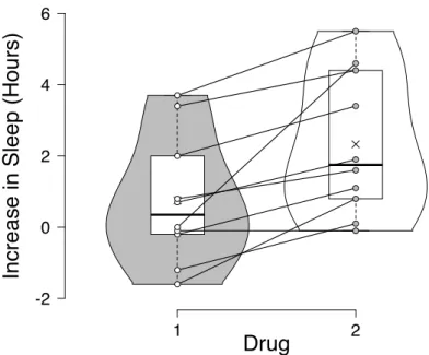
1905) which contains measurements for the effect of two soporific drugs on ten patients. Two different drugs where administered to the same ten patients and the dependent measure was the average number of hours of sleep gained compared to a control night in which no drug was administered. Figure3shows the increase in sleep (in hours) of the ten patients for each of the two drugs. To test whether the two drugs differ in effectiveness, we can conduct a Bayesian paired-samples t-test. The null hypothesis H0 states that the n difference scores di, i = 1,2, . . . , n, where n = 10, follow a normal distribution with mean zero and variance
σ2, that is, di ∼ N(0, σ2). The alternative hypothesis H1 states that the difference scores follow a normal distribution with meanµ=σδ, whereδ denotes the standardized effect size,
1 2 -2 0 2 4 6
Increase in Sleep (H
ours)
Drug
Figure 3: The sleep data set (Cushny and Peebles 1905). The left violin plot displays the distribution of the increase in sleep (in hours) of the ten patients for the first drug, the right violin plot displays the distribution of the increase in sleep (in hours) of the ten patients for the second drug. Boxplots and the individual observations are superimposed. Observations for the same participant are connected by a line. Figure also available athttps://tinyurl. com/yalskr23.
and varianceσ2, that is,di∼ N(σδ, σ2). Jeffreys’s prior is assigned to the varianceσ2 so that
p(σ2)∝1/σ2 and a zero-centered Cauchy prior with scale parameterr = 1/√2 is assigned to the standardized effect sizeδ (for details, seeRouder et al. 2009; Ly et al.2016;Morey and
Rouder 2018).
In this example, we are interested in computing the Bayes factor BF10 which quantifies how much more likely the data are under H1 (i.e., there is a difference between the two drugs)
than underH0(i.e., there is no difference between the two drugs) by using thebridgesampling package. For this example, the Bayes factor can also be easily computed using theBayesFactor package (Morey and Rouder 2018), allowing us to compare the results from thebridgesampling package to the correct answer.
The first step is to obtain posterior samples. In this example, we useJAGSin order to sample
from the models. Here we focus on how to compute the log marginal likelihood forH1. The
steps for obtaining the log marginal likelihood forH0 are analogous. After having specified the model corresponding to H1 as the character string code_H1, posterior samples can be obtained using theR2jagspackage (Su and Yajima 2015) as follows:8
R> library("R2jags")
R> data("sleep", package = "datasets") R> y <- sleep$extra[sleep$group == 1] R> x <- sleep$extra[sleep$group == 2]
8
The complete code (including theJAGS models and the code for H0) can be found in the supplemental material and also on the Open Science Framework:https://osf.io/3yc8q/.
R> d <- x - y R> n <- length(d) R> set.seed(1)
R> jags_H1 <- jags(data = list(d = d, n = n, r = 1 / sqrt(2)), + parameters.to.save = c("delta", "inv_sigma2"),
+ model.file = textConnection(code_H1), n.chains = 3,
+ n.iter = 16000, n.burnin = 1000, n.thin = 1)
Note the relatively large number of posterior samples; reliable estimates for the quantities of interest in testing usually necessitate many more posterior samples than are required for estimation. As a rule of thumb, we suggest that testing requires about an order of magnitude more posterior samples than estimation.
Next, we need to specify a function that take as input a named vector with parameter values and a data object, and returns the log of the unnormalized posterior density (i.e., the log of the integrand in Equation4). This function is easily specified by inspecting theJAGSmodel.
As a heuristic, one only needs to consider the model code where a “∼” sign appears. The
log of the densities on the right-hand side of these “∼” symbols needs to be evaluated for the
relevant quantities and then these log density values are summed.9 Using this heuristic, we obtain the following unnormalized log posterior density function forH1:
R> log_posterior_H1 <- function(pars, data) { + delta <- pars["delta"]
+ inv_sigma2 <- pars["inv_sigma2"]
+ sigma <- 1 / sqrt(inv_sigma2)
+ out <- dcauchy(delta, scale = data$r, log = TRUE) +
+ dgamma(inv_sigma2, 0.0001, 0.0001, log = TRUE) +
+ sum(dnorm(data$d, sigma * delta, sigma, log = TRUE))
+ return(out)
+ }
The final step before we can compute the log marginal likelihoods is to specify named vectors with the parameter bounds:
R> lb_H1 <- rep(-Inf, 2) R> ub_H1 <- rep(Inf, 2)
R> names(lb_H1) <- names(ub_H1) <- c("delta", "inv_sigma2") R> lb_H1[["inv_sigma2"]] <- 0
The log marginal likelihood for H1 can then be obtained by calling the bridge_sampler
function as follows:
R> library("bridgesampling") R> set.seed(12345)
R> bridge_H1 <- bridge_sampler(samples = jags_H1,
+ log_posterior = log_posterior_H1,
+ data = list(d = d, n = n, r = 1 / sqrt(2)),
+ lb = lb_H1, ub = ub_H1)
9
This heuristic assumes that the model does not include other random quantities that are generated during sampling, such as posterior predictives.
We obtain:
R> bridge_H1
Bridge sampling estimate of the log marginal likelihood: -27.17103 Estimate obtained in 5 iteration(s) via method "normal".
Note that by default, the"normal"bridge sampling method is used.
Next, we can use theerror_measuresfunction to obtain an approximate percentage error of
the estimate:
R> error_measures(bridge_H1)$percentage
[1] "0.087%"
The small approximate percentage error indicates that the marginal likelihood has been esti-mated reliably. As mentioned before, we can use thesummarymethod to obtain a convenient
summary of the bridge sampling estimate and the estimation error. We obtain:
R> summary(bridge_H1)
Bridge sampling log marginal likelihood estimate (method = "normal", repetitions = 1):
-27.17103
Error Measures:
Relative Mean-Squared Error: 7.564225e-07 Coefficient of Variation: 0.0008697255 Percentage Error: 0.087%
Note:
All error measures are approximate.
After having computed the log marginal likelihood estimate for H0 in a similar fashion, we can compute the Bayes factor forH1 overH0 using thebf function:
R> bf(bridge_H1, bridge_H0)
Estimated Bayes factor in favor of bridge_H1 over bridge_H0: 17.26001
Hence, the observed data are about 17 times more likely underH1 (which assigns the
stan-dardized effect size δ a zero-centered Cauchy prior with scale r = 1/√2) than under H0
(which fixes δ to zero). This is strong evidence for a difference in effectiveness between the two drugs (Jeffreys 1939, Appendix I). The estimated Bayes factor closely matches the Bayes factor obtained with the BayesFactor package (i.e., BF10= 17.259).
4. A “black box”
Stan
interface
The previous section demonstrated how thebridgesampling package can be used to estimate the marginal likelihood for models coded inJAGS. For custom samplers, the steps needed to
compute the marginal likelihood are the same. What is required is (a) an object with posterior samples; (b) a function that computes the log of the unnormalized posterior density; (c) the data; and (d) parameter bounds. A crucial step is the specification of the unnormalized log posterior density function. For applied researchers, this step may be challenging and error-prone, whereas for experienced statisticians it might be tedious and cumbersome, especially for complex models with a hierarchical structure.
In order to facilitate the computation of the marginal likelihood even further, the bridgesam-pling package contains an interface to the generic sampling software Stan (Carpenter et al.
2017). Assisted by the rstan package (Stan Development Team 2016a), this interface allows users to skip steps (b)–(d) above. Specifically, users who fit their models inStan(in a way that
retains the constants, as is detailed below) can obtain an estimate of the marginal likelihood by simply passing thestanfit object to thebridge_sampler function.
The implementation of this “black box” functionality profited from the fact that, just as thebridgesampling package,Stan’s No-U-Turn sampler internally operates on unconstrained
parameters (Hoffman and Gelman 2014;Stan Development Team 2017). Therstan package provides access to these unconstrained parameters and the corresponding log of the unnor-malized posterior density. This means that users can fit models with parameter types that have more complicated constraints than those currently built into bridgesampling (e.g., co-variance/correlation matrices) without having to hand-code the appropriate transformations. As mentioned above, in order to use thebridgesampling package in combination with Stan
the models need to be implemented in a way that retains the constants. This can be achieved relatively easily: instead of writing, for instance, y ~ normal(mu, sigma) or y ~ bernoulli(theta), one needs to write
target += normal_lpdf(y | mu, sigma);
and
target += bernoulli_lpmf(y | theta);
That is, one starts with the fixed expressiontarget += which is then followed by the name
of the distribution (e.g., normal). The name of the distribution is followed by _lpdf for
continuous distributions and _lpmf for discrete distributions. Finally, in parentheses, there
is the variable that was to the left of the “~” sign (here, y), then a “|” sign, and finally the
arguments of the distribution. This achieves that the user specifies the log target density (in this case, the log of the unnormalized posterior density) in a way that retains the constants of the involved distributions.
Note that in case the distributions are truncated, the user needs to code the correct renormal-ization. For instance, a normal distribution with upper truncation atupper is implemented
as follows
where the functionnormal_lcdfyields the log of the cumulative distribution function (cdf)
of the normal distribution. Likewise, a normal distribution with lower truncation atloweris
obtained as
target += normal_lpdf(y | mu, sigma) - normal_lccdf(lower | mu, sigma);
where normal_lccdf yields the log of the complementary cumulative distribution function
(ccdf) of the normal distribution (i.e., the log of one minus the cumulative distribution function of the normal distribution). A normal distribution with lower truncation point lower and
upper truncation pointupper can be implemented as follows: target += normal_lpdf(y | mu, sigma)
-log_diff_exp(normal_lcdf(upper | mu, sigma), normal_lcdf(lower | mu, sigma));
where log_diff_exp(a, b) is a numerically more stable version of the operation
log (exp (a)−exp (b)). Note that when implementing a truncated distribution, it is of course also important to give the variable of interest the correct bounds. For instance, for the last example where y has a lower truncation at lower and an upper truncation at upper the
variable yshould be declared as10
real<lower = lower, upper = upper> y;
For more details about how to implement truncated distributions inStan we refer the user to
theStanmanual (StanDevelopment Team 2017, Section 5.3, “Truncated Distributions”).
In sum, the bridgesampling package enables users to obtain an estimate of the marginal likelihood for any Stan model (programmed to retain the constants) simply by passing the
stanfit object to the bridge_sampler function. Next we demonstrate this functionality
using two prototypical examples in Bayesian model selection. 4.1. Stan example 1: Bayesian GLMM
The first example features a generalized linear mixed model (GLMM) applied to the turtles data set (Janzen, Tucker, and Paukstis 2000).11 This data set is included in the bridgesam-plingpackage and contains information about 244 newborn turtles from 31 different clutches. For each turtle, the data set includes information about survival status (0 = died, 1 = survived), birth weight in grams, and clutch (family) membership (indicated by a number between one and 31). Figure4 displays a scatterplot of clutch membership and birth weight. The clutches have been ordered according to mean birth weight. Dots indicate turtles who survived and red crosses indicate turtles who died. This data set has been analyzed in the context of Bayesian model selection before, allowing us to compare the results from the bridgesampling package to the results reported in the literature (e.g., Sinharay and Stern 2005; Overstall and Forster 2010). Here we focus on the model comparison that was
con-10
Note that we assumed thatyis a scalar. In general,ycould also be declared as a vector or an array inStan. In this case, the term that is subtracted for renormalization would need to be multiplied by the number of elements ofy. For example, for the case of an upper truncation and a vectoryof lengthkthe code would need to be changed to: target += normal_lpdf(y | mu, sigma) - k * normal_lcdf(upper | mu, sigma);For another example, see the code for “Stanexample 2”.
11
Data were obtained fromOverstall and Forster(2010) and made available in thebridgesamplingpackage with permission from the original authors.
0 5 10 15 20 25 30 35 Clutch Identifier 3 4 5 6 7 8 9
Birth Weight (Grams
)
Figure 4: Data for 244 newborn turtles (Janzen et al. 2000). Birth weight is plotted against
clutch membership. The clutches have been ordered according to their mean birth weight. Dots indicate turtles who survived and red crosses indicate turtles who died. Figure inspired bySinharay and Stern (2005). Figure also available at https://tinyurl.com/yagfxrbw. ducted in Sinharay and Stern (2005). The data set was analyzed using a probit regression model of the form:
yi ∼ B(Φ(α0+α1xi+bclutchi)), i= 1,2, . . . , N
bj ∼ N(0, σ2), j= 1,2, . . . , C,
(11) whereyi denotes the survival status of thei-th turtle (i.e., 0 = died, 1 = survived),xidenotes
the birth weight (in grams) of thei-th turtle, clutchi ∈ {1,2, . . . , C}, i= 1,2, . . . , N, indicates
the clutch to which the i-th turtle belongs, C denotes the number of clutches, and bclutchi
denotes the random effect for the clutch to which thei-th turtle belongs. Furthermore, Φ(·)
denotes the cumulative distribution function (cdf) of the normal distribution. Sinharay and Stern (2005) investigated the question whether there is an effect of clutch membership, that is, they tested the null hypothesis H0 : σ2 = 0. The following priors where assigned to the model parameters:
α0∼ N(0,10), α1∼ N(0,10),
p(σ2) =1 +σ2−2.
(12) Sinharay and Stern (2005) computed the Bayes factor in favor of the null hypothesis H0 : σ2 = 0 versus the alternative hypothesis H1 : p(σ2) = 1 +σ2
−2
using different methods and they reported a “true” Bayes factor of BF01 = 1.273 (based on extensive numerical integration). Here we examine the extent to which we can reproduce the Bayes factor using thebridgesamplingpackage.
After having implemented the Stan models as character strings H0_code and H1_code, the
next step is to run Stanand obtain the posterior samples:12
12The complete code can be found in the supplemental material, on the Open Science Framework (
https:// osf.io/3yc8q/), and is also available at?turtles. Note that the results are dependent on the compiler and the optimization settings. Thus, even with identical seeds results can differ slightly from the ones reported here.
R> library("bridgesampling") R> library("rstan")
R> data("turtles", package = "bridgesampling") R> set.seed(1)
R> stanfit_H0 <- stan(model_code = H0_code,
+ data = list(y = turtles$y, x = turtles$x, N = nrow(turtles)),
+ iter = 15500, warmup = 500, chains = 4, seed = 1)
R> stanfit_H1 <- stan(model_code = H1_code,
+ data = list(y = turtles$y, x = turtles$x, N = nrow(turtles),
+ C = max(turtles$clutch), clutch = turtles$clutch),
+ iter = 15500, warmup = 500, chains = 4, seed = 1)
With these Stan objects in hand, estimates of the log marginal likelihoods are obtained by
simply passing the objects to thebridge_sampler function:
R> set.seed(1)
R> bridge_H0 <- bridge_sampler(stanfit_H0) R> bridge_H1 <- bridge_sampler(stanfit_H1)
The Bayes factor in favor ofH0 overH1 can then be obtained as follows:
R> bf(bridge_H0, bridge_H1)
Estimated Bayes factor in favor of bridge_H0 over bridge_H1: 1.27151
This value is close to that of 1.273 reported inSinharay and Stern(2005). The data are only slightly more likely underH0 than underH1, suggesting that the data do not warrant strong
claims about whether or not clutch membership affects survival.
The precision of the estimates for the marginal likelihoods can be obtained as follows:
R> error_measures(bridge_H0)$percentage
[1] "0.00972%"
R> error_measures(bridge_H1)$percentage
[1] "0.348%"
These error percentages indicate that both marginal likelihoods have been estimated accu-rately, but – as expected – the marginal likelihood for the more complicated model with random effects (i.e.,H1) has the larger estimation error.
4.2. Stan example 2: Bayesian factor analysis
The second example concerns Bayesian factor analysis. In particular, we determine the num-ber of relevant latent factors by implementing the Bayesian factor analysis model proposed byLopes and West(2004). The model assumes that there aret, t= 1,2, . . . , T, observations
on each ofmvariables. That is, each observationytis anm-dimensional vector. Thek-factor
model – where k denotes the number of factors – relates each of the T observations yt to
a latent k-dimensional vector ft which contains for observation t the values on the latent
factors, as follows:13
yt|ft∼ Nm(βft,Σ)
ft∼ Nk(0k,Ik),
(13) where β denotes the m×k factor loadings matrix14, Σ= diag σ21, σ22, . . . , σm2
denotes the m×mdiagonal matrix with residual variances,0k denotes ak-dimensional vector with zeros,
and Ik denotes the k×k identity matrix. Hence, conditional on the latent factors, the
observations on themvariables are assumed to be uncorrelated with each other. Marginally, however, the observations are usually not uncorrelated and they are distributed as
yt∼ Nm(0m,Ω), (14)
where Ω =ββ>+ Σ. Here we reanalyze a data set that contains the changes in monthly
international exchange rates for pounds sterling from January 1975 to December 1986 (West and Harrison 1997, pp. 612–615). Currencies tracked are US Dollar (US), Canadian Dollar (CAN), Japanese Yen (JAP), French Franc (FRA), Italian Lira (ITA), and the (West) German Mark (GER). Figure5displays the data.15 Using different computational methods, including bridge sampling, Lopes and West (2004) estimated the marginal likelihoods and posterior model probabilities for a factor model with one, two, and three factors. As before, this allows us to compare the results from the bridgesampling package to the results reported in the literature. To identify the model, the factor loading matrix β is constrained to be lower-triangular (Lopes and West 2004). The diagonal elements of β are constrained to be positive by assigning them standard half-normal priors with lower truncation point zero: βjj ∼ N(0,1)T(0,), j = 1,2, . . . , k, and the lower-diagonal elements are assigned standard normal priors. The residual variances are assigned inverse-gamma priors of the form σi2 ∼
Inverse-Gamma(ν/2, νs2/2), i = 1,2, . . . , m, where ν = 2.2 and νs2 = 0.1 (for details, see Lopes and West 2004).
The first step in our reanalysis is to specify theStanmodel as the character stringmodel_code.
We can then fit the three models corresponding tok= 1,k= 2, andk= 3 latent factors and estimate the log marginal likelihoods usingbridgesamplingas follows:16
R> library("rstan")
R> library("bridgesampling")
R> data("ier", package = "bridgesampling") 13
Note that the model assumes that the observations are zero-centered.
14We use the original notation byLopes and West (2004) who denoted the factor loadings matrix with a lower-case letter. In the remainder of the article, matrices are denoted by upper-case letters.
15Each series has been standardized with respect to its sample mean and standard deviation. These stan-dardized data are included in thebridgesamplingpackage.
16The complete code can be found in the supplemental material, on the Open Science Framework (https:
//osf.io/3yc8q/), and is also available at?ier. Note that we specify initial values using a custominit_fun
function. This function may need to be changed for different applications. Furthermore, it is strongly advised to check that the chains have indeed converged since we sometimes encountered convergence issues with this model. Note that the results are dependent on the compiler and the optimization settings. Thus, even with identical seeds results can differ slightly from the ones reported here.
1975 1978 1981 1984 1987 -4 -2 0 2 4 Year
Exchange Rate Changes
US Dollar 1975 1978 1981 1984 1987 -4 -2 0 2 4 Year
Exchange Rate Changes
Canadian Dollar 1975 1978 1981 1984 1987 -4 -2 0 2 4 Year
Exchange Rate Changes
Yen 1975 1978 1981 1984 1987 -4 -2 0 2 4 Year
Exchange Rate Changes
Franc 1975 1978 1981 1984 1987 -4 -2 0 2 4 Year
Exchange Rate Changes
Lira 1975 1978 1981 1984 1987 -4 -2 0 2 4 Year
Exchange Rate Changes
Mark
Figure 5: Changes in monthly international exchange rates for pounds sterling from January 1975 to December 1986 (West and Harrison 1997, pp. 612–615). Currencies tracked are US Dollar (US), Canadian Dollar (CAN), Japanese Yen (JAP), French Franc (FRA), Italian Lira (ITA), and the (West) German Mark (GER). Each series has been standardized with respect to its sample mean and standard deviation. Figure reproduced fromLopes and West(2004). Figure also available athttps://tinyurl.com/ybtdddyv.
R> cores <- 4
R> options(mc.cores = cores)
R> model <- stan_model(model_code = model_code) R> set.seed(1)
R> stanfit <- bridge <- vector("list", 3) R> for (k in 1:3) {
+ stanfit[[k]] <- sampling(model,
+ data = list(Y = ier, T = nrow(ier), m = ncol(ier), k = k),
+ iter = 11000, warmup = 1000, chains = 4,
+ init = init_fun(nchains = 4, k = k, m = ncol(ier)),
+ bridge[[k]] <- bridge_sampler(stanfit[[k]], method = "warp3",
+ repetitions = 10, cores = cores)
+ }
Note that in this example, we use the "warp3" method instead of the "normal" method.
Furthermore, since the error_measures function cannot be used when the estimate has
been obtained using method = "warp3" with repetitions = 1, we set repetitions = 10
to obtain an empirical estimate of the estimation uncertainty (conditional on the posterior samples). We also select parallel computation by setting cores = 4. The summary method
provides a convenient overview of the estimate and the estimation uncertainty. For instance, for the 2-factor model, we obtain as output:
R> summary(bridge[[2]])
Bridge sampling log marginal likelihood estimate (method = "warp3", repetitions = 10):
-903.4522 Error Measures: Min: -903.4565 Max: -903.4481 Interquartile Range: 0.002682305 Note:
All error measures are based on 10 estimates.
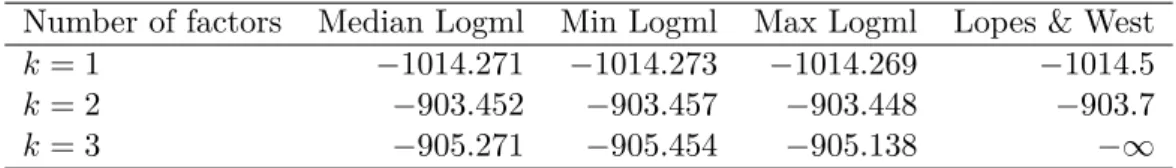
Table 4.2 displays for each of the three factor models (i.e., k= 1,k = 2,k= 3) the median log marginal likelihood (logml) across repetitions, the minimum/maximum log marginal like-lihood across repetitions, and the log marginal likelike-lihood value reported in Lopes and West (2004) based on bridge sampling. Note that the negative infinity reported byLopes and West (2004) might be due to a numerical problem. For the 1-factor model and the 2-factor model, the log marginal likelihoods obtained viabridgesamplingare very similar to the ones reported inLopes and West(2004). Furthermore, the narrow range of the estimates indicates that the estimation uncertainty is small (conditional on the posterior samples, as described above). To examine the support for the three different models (i.e., different numbers of latent factors), we can use thepost_prob function to compute posterior model probabilities. By default, the
function assumes that all models are equally likely a priori; this can be adjusted using the
prior_prob argument. Furthermore, the model_namesargument can optionally be used to
provide names for the models. Here we use the default of equal prior model probabilities and we obtain:
R> post_prob(bridge[[1]], bridge[[2]], bridge[[3]], + model_names = c("k = 1", "k = 2", "k = 3"))
k = 1 k = 2 k = 3 [1,] 6.278942e-49 0.8435919 0.1564081
Number of factors Median Logml Min Logml Max Logml Lopes & West k= 1 −1014.271 −1014.273 −1014.269 −1014.5
k= 2 −903.452 −903.457 −903.448 −903.7 k= 3 −905.271 −905.454 −905.138 −∞
Table 2: Log marginal likelihood (logml) estimates for the k = 1, k = 2, and k = 3 factor model. The rightmost column displays the values based on bridge sampling reported inLopes and West (2004). [2,] 6.309963e-49 0.8491811 0.1508189 [3,] 6.373407e-49 0.8554668 0.1445332 [4,] 6.511718e-49 0.8739641 0.1260359 [5,] 6.582895e-49 0.8805172 0.1194828 [6,] 6.384273e-49 0.8596401 0.1403599 [7,] 6.469723e-49 0.8736989 0.1263011 [8,] 6.403270e-49 0.8616183 0.1383817 [9,] 6.426132e-49 0.8635907 0.1364093 [10,] 6.417346e-49 0.8592737 0.1407263
Each row presents the posterior model probabilities based on one repetition of the bridge sampling procedure for all three models (i.e., each row sums to one). Hence, there are as many rows as repetitions.17 The 2-factor model receives most support from the observed
data. This is in line with Lopes and West (2004), who also preferred the 2-factor model;18 based on the factor loadings, they proposed the presence of a North American factor and a European Union factor.
5. Discussion
This paper introduced bridgesampling, an R package for computing marginal likelihoods,
Bayes factors, posterior model probabilities, and normalizing constants in general. We have demonstrated how researchers can usebridgesamplingto conduct Bayesian model comparisons in a generic, user-friendly way: researchers need only provide posterior samples, a function that computes the log of the unnormalized posterior density, the data, and lower and upper bounds for the parameters. Furthermore, we have described theStaninterface which makes it
even easier to obtain the marginal likelihood: researchers need only provide astanfitobject
and the bridgesampling package will automatically produce an estimate of the log marginal likelihood.19 In other words, thebridgesamplingpackage makes it possible to obtain marginal
17
Note that the output of the post_probfunction can be directly passed to the boxplot function which allows one to visualize the estimation uncertainty in the posterior model probabilities across repetitions.
18
Note thatLopes and West(2004) report a posterior model probability of 1 for the 2-factor model. However, this estimate may be inflated by the infinite log marginal likelihood value for the 3-factor model.
19
Similar to the ‘stanfit’ method, thebridge_samplermethod fornimbleonly requires the fitted object (of class ‘MCMC_refClass’) and extracts all necessary information for computing the marginal likelihood (including the function for computing the unnormalized log posterior density and the parameter bounds). However, at the time of writing we have not yet tested this method in the same intensity as the ‘stanfit’ method. We will add a vignette describing thenimbleinterface in more detail when we have done so.
likelihood estimates for any model that can be implemented inStan(in a way that retains the
constants). By combining theStan state-of-the-art No-U-Turn sampler withbridgesampling, researchers are provided with a general purpose, easy-to-use computational solution to the challenging task of comparing complex Bayesian models.
As practical advice, we recommend to keep the following four points in mind when using the bridgesampling package (see also Gronau et al. 2020a, 2019). First, one should always
check the posterior samples carefully. A successful application of bridge sampling requires a sufficient number of representative samples from the posterior distribution. Thus, it is im-portant to use efficient sampling algorithms and, in case of MCMC sampling, it is crucial that researchers confirm that the chains have converged to the joint posterior distribution. In addition, researchers need to make sure that the model does not contain any discrete pa-rameters since those are currently not supported. This may sound more restrictive than it is. In practice the solution is to marginalize out the discrete parameters, something that is often possible. Note the similarity toStan which also deals with discrete parameters by
marginal-izing them out (Stan Development Team 2017, Section 15). Furthermore, as demonstrated in the examples, for conducting model comparisons based on bridge sampling, the number of posterior samples often needs to be an order of magnitude larger than for estimation. This of course depends on a number of factors such as the complexity of the model of interest, the number of posterior samples that one usually uses for estimation, the posterior sampling algorithm used, and also the accuracy of the marginal likelihood estimate that one desires to achieve.
Second, one should always assess the uncertainty of the bridge sampling estimate. In case the uncertainty is deemed too high, one can attempt to achieve a higher precision by increasing the number of posterior samples or, in casemethod = "normal", by using the more
sophis-ticatedmethod = "warp3" instead (see the third point below). Users of thebridgesampling package have different options for assessing the estimation uncertainty. In our opinion, the “gold standard” may be to obtain an empirical uncertainty assessment by repeating the bridge sampling procedure multiple times, each time using a fresh set of posterior samples. This ap-proach allows users to assess the uncertainty directly for the quantity of interest. For instance, if the focus is on computing a Bayes factor, users may repeat the following steps: (a) obtain posterior samples for both models, (b) use thebridge_samplerfunction to estimate the log
marginal likelihoods, (c) compute the Bayes factor using thebf function. The variability of
these Bayes factor estimates across repetitions then provides an assessment of the uncertainty. For certain applications, this approach may be infeasible due to computational restrictions. If this is the case and method = "normal", we recommend to use the approximate errors
based onFrühwirth-Schnatter(2004) which are available through theerror_measures
func-tion. As mentioned before, we have found these approximate errors to work well formethod = "normal", but not for method = "warp3" which is the reason why they are not available
for the latter method. Alternatively, one can also assess the estimation uncertainty by setting therepetitionsargument to an integer larger than one. This provides an assessment of the
estimation uncertainty due to variability in the samples from the proposal distribution, but it should be kept in mind that this does not take into account variability in the posterior samples.
Third, one should consider whether using the more time-consuming Warp-III method may be beneficial. The accuracy of the estimate is governed not only be the number of samples, but also by the overlap between the posterior and the proposal distribution (e.g.,Meng and
Wong 1996;Meng and Schilling 2002). The bridgesampling package attempts to maximize this overlap by (a) focusing on one marginal likelihood at a time which allows one to use a convenient proposal distribution which closely resembles the posterior distribution, (b) using a proposal distribution which matches the mean vector and covariance matrix of the posterior samples (i.e.,method = "normal") or additionally also the skewness (i.e.,method = "warp3"). Consequently, as mentioned before, method = "warp3" will always be as precise
or more precise than method = "normal"; however, it also takes about twice as long. We
have found that in many applications, method = "normal"works well, however, in case the
posterior is skewed (crucially, this refers to the joint posterior of the quantities that have been transformed to the real line), method = "warp3" may be the better choice. When in
doubt, we believe that it may be beneficial to also explore the Warp-III results – if this is computationally feasible – to see how much (if any) improvement in precision is achieved by taking into account potential skewness. It should be kept in mind that, in case the posterior distribution exhibits multiple modes, the overlap of the two distributions may still be subject to improvement – even when using method = "warp3". The development of efficient bridge
sampling variants for these cases is subject to ongoing research (e.g.,Wang and Meng 2016; Frühwirth-Schnatter 2004).
Forth, users should carefully think about the choice of prior distribution. Even though the bridgesamplingpackage enables researchers to compute the marginal likelihoods in an almost black-box manner, this does not imply that the user can mindlessly exploit the package func-tionality to conduct Bayesian model comparisons. As is apparent from Equation4, Bayesian model comparisons depend on the choice of the parameter prior distribution. Crucially, the prior distribution has a lasting influence on the results. Hence, meaningful Bayesian model comparisons require that researchers carefully consider their parameter prior distribution (e.g., Lee and Vanpaemel 2018), engage in sensitivity analyses, or use default prior choices that have certain desirable properties such as model selection and information consistency (e.g.,Jeffreys 1961;Bayarri, Berger, Forte, and García-Donato 2012;Lyet al.2016).20 Thus,
the bridgesampling package removes the computational hurdle of obtaining the marginal likelihood, thereby allowing researchers to spend more time and effort on the specification of meaningful prior distributions.
It should also be kept in mind that there may be cases in which the bridge sampling procedure may not be the ideal choice for conducting Bayesian model comparisons. For instance, when the models are nested it might be faster and easier to use the Savage-Dickey density ratio (Dickey and Lientz 1970;Wagenmakers, Lodewyckx, Kuriyal, and Grasman 2010). Another example is when the comparison of interest concerns a very large model space, and a separate bridge sampling based computation of marginal likelihoods may take too much time. In this scenario, reversible jump MCMC (Green 1995) may be more appropriate. The downside of reversible jump MCMC is that it is usually problem-specific and cannot easily be applied in a generic fashion to different nested and non-nested model comparison problems (but see Gelling et al.2017). The goal with the bridgesampling package, however, was exactly that: to provide users with a generic way of computing marginal likelihoods which can in principle be applied to any Bayesian model comparison problem.
In the future, we hope that it may be possible to addbridgesampling support for a number
20Note that in the first example (i.e., the Bayesian t-test) we have used prior distributions which lead to these desirable properties. However, in the second and third example, we simply used the prior distributions that have been used in the literature so that we could compare our results to the reported results.
of R packages, such as the MCMCglmm package (Hadfield 2010), the JAGS interface of
the mgcv package (Wood 2016), the glmmBUGS package (Brown and Zhou 2018), or the blavaan21 package (Merkle and Rosseel 2018) so that users could conduct Bayesian model comparisons in a black box way similar to theStaninterface. For packages that use themselves Stan for fitting the models, adding bridgesamplingsupport is relatively straightforward: the only potential change that would have to be implemented is to make sure that the models are coded such that all constants are retained (as explained in section 4). Once this is achieved, computing the relevant quantities via bridgesampling works as described in the
Stan examples. For packages that do not use Stan to fit the models, the main difficulty
is specifying the unnormalized posterior density function and the parameter bounds in an automatized way. This is also the reason why there is currently no black box interface to
JAGSsince, to the best of our knowledge, specifying these quantities in an automatized way
is not trivial. Nevertheless, if this hurdle could be overcome, addingbridgesampling support would be straightforward.
In sum, the bridgesampling package provides a generic, accurate, easy-to-use, automatic, and fast way of computing marginal likelihoods and conducting Bayesian model comparisons. With the computational challenge all but overcome, researchers can spend more time and effort on addressing the conceptual challenge that comes with Bayesian model comparisons: specifying prior distributions that are either robust or meaningful.
Acknowledgments
This research was supported by a Netherlands Organisation for Scientific Research (NWO) grant to QFG (406.16.528), by an NWO Vici grant to EJW (016.Vici.170.083), and by the Berkeley Initiative for Transparency in the Social Sciences, a program of the Center for Effective Global Action (CEGA), with support from the Laura and John Arnold Foundation.
References
Bayarri MJ, Berger JO, Forte A, García-Donato G (2012). “Criteria for Bayesian Model Choice with Application to Variable Selection.” The Annals of Statistics, 40(3), 1550–
1577. doi:10.1214/12-aos1013.
Brown PE, Zhou L (2018). glmmBUGS: Generalised Linear Mixed Models and Spatial Models with WinBUGS, JAGS, and OpenBUGS. R package version 2.4.2, URL https://CRAN. R-project.org/package=glmmBUGS.
Carlin BP, Chib S (1995). “Bayesian Model Choice via Markov Chain Monte Carlo Methods.” Journal of the Royal Statistical Society B, 57(3), 473–484. doi:10.1111/j.2517-6161. 1995.tb02042.x.
Carpenter B, Gelman A, Hoffman M, Lee D, Goodrich B, Betancourt M, Brubaker M, Guo J, Li P, Riddell A (2017). “Stan: A Probabilistic Programming Language.” Journal of Statistical Software,76(1), 1–32. doi:10.18637/jss.v076.i01.
21
Note that theblavaanpackage already provides approximate marginal likelihoods for the models that are obtained via a Laplace approximation.