Learning to Generate 3D Training Data

(1)

Learning to Generate 3D Training Data

by

Dawei Yang

A dissertation submitted in partial fulfillment of the requirements for the degree of

Doctor of Philosophy

(Computer Science and Engineering) in the University of Michigan

2020

Doctoral Committee:

Professor Jia Deng, Co-Chair, Princeton University Assistant Professor David F. Fouhey, Co-Chair Professor Vineet R. Kamat

(2)

Dawei Yang ydawei@umich.edu

ORCID iD: 0000-0003-0799-5234 © Dawei Yang 2020

(3)

(4)

ACKNOWLEDGMENTS

First of all, I would like to thank my parents, Yang Zhengwang and Weng Donghua, who have been supporting me unconditionally since I started kinder-garten. Further, I would like to thank my advisor Prof. Jia Deng, for his enthusiasm for the projects, for his continuous support and guidance during this research. I also wish to express my appreciation for Prof. Shi-Min Hu and Prof. Kun Xu, who advised me during my undergraduate years. Finally, special thanks to all members of the dissertation committee, Prof. Jia Deng, Prof. David Fouhey, Prof. Vineet Kamat and Prof. Benjamin Kuipers, for thoughtful com-ments and recommendations on this dissertation.

(5)

LIST OF FIGURES

2.1 The overview of our approach. Starting from simple primitives such as spheres and cubes, we evolve a population of complex shapes. We render synthetic images from the shapes to incrementally train a shape-from-shading network. The performance of the network on a validation set of real images is then used to guide the shape evolution. 14 2.2 The computation graphs of four primitive shapes defined in Equation 2.1. The unlabeled

edge weight and node bias are0, and the unlabeled reduction function issum. . . 18 2.3 Shape transformation represented by graph operation. Left: the graph of the shape

before transformation. Right: the graph of the shape after transformation. . . 18 2.4 The union of two shapes represented by graph merging. Left: the respective graphs of

the two shapes to be unioned. Right: the graph of the unioned shape. . . 19 2.5 Evolution towards a target shape. Left: targets. Right: The fittest shapes in the

population as the evolution progresses at different iterations. . . 23 2.6 The best IoU with the target shape (heart) versus evolution time (top) and the number

of iterations (bottom) for different combinations of design choices. . . 24 2.7 The qualitative results of our method and SIRFS [8] on the test data. . . 29 2.8 Example shapes at different stages of the evolution and shapes from ShapeNet. . . 29 3.1 Our hybrid gradient method. We parametrize the design decisions as a real vectorβ

and optimize the function of performanceLwith respect toβ. Fromβto the generated

training images and ground truth, we compute the approximate gradient by averaging finite difference approximations. From training samples X to L, we compute the

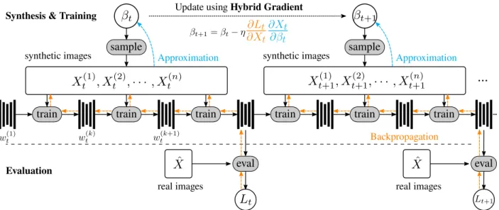
analytical gradient through backpropagation with unrolled training steps. . . 31 3.2 The details of using “hybrid gradient” to incrementally updateβand train the network.

The analytical gradient is computed by backpropagating through unrolled training steps (colored in orange). The numerical gradient is computed using finite difference approximation by sampling in a neighborhood of βt (colored in cyan). Then βt is

updated using hybrid gradient, and the trained network weights are retained for the next timestampt+ 1. . . 38 3.3 Sampled shapes from our probabilistic context-free grammar, with parameters

opti-mized using hybrid gradient. . . 42 3.4 Mean angle error on the test imagesvs. computation time, compared to two black-box

optimization baselines. . . 43 3.5 Training images generated using PCFG with 3DMM face model, and example test

(8)

3.6 Example textures generated using our procedural pipeline with parameters controlled byβ. . . 47

4.1 The overview of our method. We evolve a set of 3D configurations as genomes, with fitness scores defined as novelty. The genomes are first rendered into synthetic images. The novelty is then computed by applying a deep autoregressive model to calculate bits/subpixel for encoding the image. This indicates how novel a genome is in terms of previously seen images. . . 53 4.2 The most and least novel shapes at different epochs in the evolution process. The

PixelCNN trained on synthetic shapes is able to assign a low novelty score for primitive shapes such as spheres and cubes, and assign a high score for interesting compositions. Top left: input image Top left: input image. (Top right: visualization of ground truth normals. Bottom left: mask. Bottom right: novelty score.) . . . 62 4.3 The fitness distribution changes over time. Different shades represent minimum,

maximum and25%,50%,75%percentiles. . . 62 4.4 The trajectory of training PixelCNN over time. . . 62 4.5 Randomly sampled scenes in the initial population. The objects and randomly placed

inside a cube with background textures. The light sources are point lights with random locations and color intensity. . . 62 4.6 The novelty scores for novel random scenes. It learns to assign trivial cases with a low

score, such as occluded cameras or degraded lighting. . . 62 A.1 The test set of the MIT-Berkeley Intrinsic Images dataset. . . 69 A.2 The original scenes in the SUNCG dataset, and our scenes with camera and objects

perturbed using our PCFG. . . 70 A.3 Training images generated using PCFG with 3DMM face model, and 6 example images

from the test set. . . 71 A.4 Our texture generation pipeline and example images of the training and test set. . . 71 A.5 How probability distributions change over time for SUNCG perturbation parameters.

The three images plot the probability densitity of shape displacement along x, y, z axes respectively.. . . 72

(9)

LIST OF TABLES

2.1 The results of baselines and our approach on the test images.∗_{Measured by uniformly} randomly outputting unit vectors on the+z hemisphere. . . 28

3.1 Ablation Study: the diagnostic experiment to compare with random but fixedβ. We

sample10values ofβ in advance, and then train the networks with the same setting

as in hybrid gradient. The best, median and worst performance is reported on the test images, and the corresponding values ofβ are used to initializeβ0 for hybrid gradient for comparison. The results show that our approach is consistently better than the baselines with fixedβ. . . 41

3.2 Our approach compared to previous work, on the test set of MIT-Berkeley images [8]. The results show that our approach is better than the state of the art as reported in Table 2.1. . . 41 3.3 The performance of the finetuned networks on the test set of NYU Depth V2 [138],

compared to the original network in [175]. The networks are trained only on the synthetic images. Without optimizing the parameters (randomβ), the augmentation

hurts the generalization performance. With proper search ofβusing hybrid gradient,

we are able to achieve better performance than the original model. . . 45 3.4 The results on the scanned faces of the Basel Face Model. Our method is able to search

for the synthetic face parameters such that the trained network can generalize better. . 46 3.5 The results of intrinsic image decomposition on the ShapeNet renderings. . . 48 4.1 The evaluation results on MBII [8]. Compared to supervised methods, we are able to

achieve reasonable results even without seeing a single image in MBII. Compared to the baseline “No novelty”, our novelty metric helps to generate novel shapes such that the trained network can generalize better on unseen images. . . 60 4.2 Results on ShapeNet [17] and Pix3D [147] renderings. We obtain the model from

[169] and directly evaluate on this dataset. The results show that the network trained on our synthetic dataset generalizes better.. . . 60

(10)

ABSTRACT

Human-level visual 3D perception ability has long been pursued by researchers in computer vision, computer graphics, and robotics. Recent years have seen an emerging line of works using synthetic images to train deep networks for single image 3D perception. Synthetic images rendered by graphics engines are a promising source for training deep neural networks because it comes with perfect 3D ground truth for free. However, the 3D shapes and scenes to be rendered are largely made manual. Besides, it is challenging to ensure that synthetic images collected this way can help train a deep network to perform well on real images. This is because graphics generation pipelines require numerous design decisions such as the selection of 3D shapes and the placement of the camera.

In this dissertation, we propose automatic generation pipelines of synthetic data that aim to improve the task performance of a trained network. We explore both supervised and unsupervised directions for automatic optimization of 3D decisions. For supervised learning, we demonstrate how to optimize 3D parameters such that a trained network can generalize well to real images. We first show that we can construct a pure synthetic 3D shape to achieve state-of-the-art performance on a shape-from-shading benchmark. We further parameterize the decisions as a vector and propose a hybrid gradient approach to efficiently optimize the vector towards usefulness. Our hybrid gradient is able to outperform classic black-box approaches on a wide selection of 3D perception tasks. For unsupervised learning, we propose a novelty metric for 3D parameter evolution based on deep autoregressive models. We show that without any extrinsic motivation, the novelty computed from autoregressive models alone is helpful. Our novelty metric can consistently encourage a random synthetic generator to produce more useful training data for downstream 3D perception tasks.

(11)

CHAPTER 1 Introduction

1.1 Background

1.1.1 Single Image 3D Perception with Deep Neural Networks

We capture our 3D world into digital images, store them on our digital devices such as cameras, phones, and computers. We print them out, view them on our display, or share them online with others. Though these images encode the 3D of the scene, they are represented in the form of 2D matrices of color values, or pixels. For humans, we are naturally good at understanding the 3D structure and recovering the 3D content inside, regardless of their 2D form. However, for computers, human-level visual 3D perception ability is not for free; such ability has long been pursued by researchers in a wide variety of fields, including computer vision, computer graphics, and robotics. In prior research, single image 3D perception generally relies on monocular cues in the image, such as shading, texture or edges. Early studies focus on those cues for 3D surface reconstruction, also known as shape-from-X. For example, one can estimate the surface normal direction from how texture patterns vary across the 2D image [32]. These studies of monocular cues base the assumptions on our knowledge of the real world, such as assumptions of smooth surfaces, uniform painting, and natural illumination [8].

Recent years have seen an emerging line of literature using data-driven approaches, specifically deep neural networks, with significant progress on the task of single image 3D recovery. Deep neural networks do away from manual specification of priors. Instead, they automatically learn the prior knowledge from a dataset of images with 3D ground truth. This largely avoids the manual design of

(12)

optimization objectives and algorithms, and instead take advantage of large-scale datasets. Deep networks have shown great promise in recovering 3D from images, with increasing state-of-the-art performance on standard benchmarks [38,74,82,70,53,44,81,113,24,71,116,176,59].

1.1.2 3D Representations in Deep Learning

For single image 3D perception, the 3D representation can take many different forms. Especially for deep learning, researchers typically cater to their needs. Here we summarize common 3D representations used in this dissertation.

3D meshes Meshes are compact surface representation describing the surface geometry using polygon faces. In deep learning, 3D polygon meshes are prevalently used for rendering synthetic images because of the easy integration with graphics rendering pipelines. It is also a standard representation in 3D modeling. Therefore, 3D mesh datasets [17,179,27,62,147] are collected for synthesizing images to train or evaluate 3D perception tasks for deep neural networks.

Depth, normal, reflectance and shading Maps For deep neural networks, 2D maps of depth and normal are common options for representing 3D structures of scenes. They are obtained by mapping the normal vector and the depth of corresponding 3D surface points at each pixel to a 2D matrix. This structured 2D representation is similar to a 2D image, so it is easier to design neural network architectures suited for pixelwise prediction. A large body of work uses this representation for designing deep neural networks for 3D tasks [38,82,70,53,44,113,24,116,59]. Compared to recovering the full 3D surface from a single image, the depth and normal maps only include the surface points that appear in the 2D image, and thus avoids the need for hallucinating the occluded parts.

Another related representation is intrinsic images, which are the reflectance and the shading components of a single image. The reflectance map contains the material color of the objects at each pixel mapped into a 2D image. Similarly, the shading map is the accumulation of lighting on the surface at each pixel. In simplified settings, the reflectance only depends on the intrinsic material

(13)

properties of the objects and does not depend on external illumination; the shading is uniquely determined by the surface geometry and external illumination. Though reflectance and shading do not directly represent a 3D surface, a 3D surface can be further extracted from those intrinsic components. Therefore, they also share the common goal of 3D perception, and frequently appear in related literature [137,177,47,9,61,88,135,79,173,134,78].

Implicit functions For 3D surface representation, an implicit function F(x, y, z) takes a 3D

coordinate (x, y, z) as input and outputs a real value. The surface is represented by the zero

level set of the function F(x, y, z). The shape surface in this form is not directly available for

rendering, unless special rendering techniques are developed [55], or the surface is explicitly extracted using algorithms such as marching cubes [85]. Recently in deep learning, implicit functions are represented using a deep neural network, sometimes conditioned on the input image for single image 3D recovery [83,168,96,26,105,50].

Constructive solid geometry Constructive solid geometry (CSG) represents a shape using a symbolic tree of primitive shapes [43]. The leaf nodes represent primitive shapes such as cylinders, cubes, spheres,etc. The non-leaf nodes specify the boolean operations such as union, intersection

and difference on their children. The final shape is computed by recursively applying the boolean operations from children to parents. Under the assumption that the objects can be composed by a set of simple primitives, researchers have also studied parsing CSG for single shape recovery [182, 136,36,149].

1.1.3 Training Datasets for Single Image 3D

Large-scale datasets such as ImageNet [35], Microsoft COCO [80] are essential for the success of deep neural networks in classification and object recognition tasks. The class label and object bounding boxes are relatively easy to annotate. However, for single image 3D, the task requires dense prediction of 3D, so sufficiently annotated 3D ground truth is often required for supervised learning of deep networks. The main approaches for acquiring 3D ground truth approximately fall

(14)

into several categories.

1.1.3.1 Manual Capturing of Real World

Depth scanned by sensors is a valid source for collecting dense 3D ground truth. A number of datasets follow this line and capture RGB-D images using Kinect or LiDAR [129,138,48,62, 139,27]. In RGB-D images, the depth map is recorded using the range sensor and then aligned to the corresponding RGB image. For example, the NYU Depth V2 dataset [138] has 407,024 RGB-D frames of indoor rooms collected using a mounted Kinect. SUN RGB-D [139] has 10,000 indoor RGB-D images along with 58,657 human-annotated bounding boxes of 3D objects. For autonomous driving scenarios, The KITTI Vision Benchmark Suite [49] includes RGB-D videos of road scenes along with many other 3D ground truths of stereo matching, optical flow, odometry and semantic segmentation.

While these large-scale datasets have shown their effectiveness in training a deep neural network to perform 3D perception tasks, capturing using sensors may be limited to sensor types and may not result in diverse data. The datasets typically target to specific scenarios such as autonomous driving [49] or indoor scenes and objects [138,139].

1.1.3.2 Manual Annotation of Internet Images

Other than sensor capturing, there is also a line of work asking human workers to annotate 3D from the internet images [22,9, 21]. For example, Chen et al. [21] exploits human’s ability of judging relative depth to collect sparse depth pairs in an image. Their followup work [22] designs an efficient UI for collecting sparsely-annotated normals.

Due to limited throughput for human-computer interaction, the annotations are expected to be sparse. In addition, human annotation may be prone to errors so quality assurance is typically needed to ensure the datasets will be relevant for training a deep neural network.

(15)

1.1.3.3 Synthetic Rendering using Graphics Engines

Graphics engines are physically accurate simulation of photo-taking in the real world. In the sim-ulation, 3D ground truth such as depth and normal maps, 3D surfaces are readily available without much additional cost. As mentioned earlier, single image 3D perception with deep neural networks rely on provided 3D ground truth for supervision. Synthetic training images rendered by graphics engines perfectly suit this scenario: they come with high-quality ground truth annotations for free, such as pixel-perfect depth, normal and intrinsic images, complete lighting condition and camera parameters. Therefore, synthetic images generated by computer graphics have been extensively used for training deep networks for numerous tasks, including single image 3D reconstruction [139, 58,95,62,171,17], optical flow estimation [94,15,46], human pose estimation [155,23], action recognition [121], visual question answering [64], and many others [114,91,164,151,119,120, 163]. The success of these works has demonstrated the effectiveness of synthetic images.

Compared to manual collection of real images, graphics rendering of synthetic images gives full flexibility and control over the scene to be rendered. This includes the selection of objects in the scene, their poses, the illumination configuration, camera intrinsics and extrinsics. The flexibility in a graphics pipeline allows free designing and modification of every piece of a scene to fit specific needs. In the context of training deep neural networks, the target is to make synthetic images better training data. This means the synthetic images need to be large-scale and relevant to 3D perception tasks.

Most of today’s existing synthetic datasets collect 3D assets with manual labor. The idea behind is similar to capturing real images: designs of 3D scenes and collection of 3D shapes can be made manual. Scenes and shapes that are designed by humans are similar to those that exist in the real world, so they are expected to be useful training data for deep neural networks. Take a popular dataset as an example, ShapeNet [17] includes 50,000+ shapes in 55 real-world categories. As for indoor scenes, SUNCG [140] contains 45,622 realistic indoor designs that are crowdsourced from an online platform. Users design artistic floor plans in a house, arrange textured furniture and other objects in the scene. Zhang et al. [175] and Li and Snavely [77] further render them for 3D tasks

(16)

and show the large-scale datasets can help a network to perform well on real indoor scenes. Similar datasets have been collected in this way, including SceneNet [95], Falling Things [152] and SceneNN [58].

To increase the number of samples and reduce human cost, we have seen a few attempts on automation of generating synthetic datasets. Manual heuristics can be seen in constructing synthetic datasets, such as [175]. They randomly generate camera locations and angles, and then filter out camera views that produce renderings with minimal pixel variety of object instances. Another example is SceneNet [95], where they use gravity to randomize object arrangements. The randomization increases the variety of the data and may potentially increase the task performance of the trained network.

1.2 Motivation

As we have seen, synthetic images rendered by graphics engines are a great source for training deep neural networks on various 3D perception tasks. However, today’s synthetic datasets still involve large manual effort. Same as manual capturing of real images, human collection involves intensive labor and considerable time for large-scale datasets. Besides, the application of synthetic training data is hindered by the reality gap: it is not clear how to make sure that the generated data will be useful for real-world tasks. Since there are only limited instances in the datasets collected this way, it is also not clear how much can be considered enough for training deep neural networks to perform well.

In this dissertation, we consider synthetic rendering pipelines aiming to solve the above problems. Specifically, we are motivated by the flexibility of synthetic scenes: since we have full control of every part of 3D content, we should make full use of this advantage. Our strategy is full automation of the decisions including shape selection, lighting environment, object arrangement and camera placementetc., while aiming at improving the quality of the dataset for training deep

(17)

1.2.1 Automating the Graphics Pipeline

Automating the generation of synthetic data can relieve manual effort of collecting data. In this dissertation, we propose methods that generate synthetic data in a fully automatic fashion, with minimal manual design involved. For each task scenario, we first design a minimal template for it. For example, for single shape from shading, we assume there is one single object and a global illumination model in the scene. For human face reconstruction, we assume a face model is used with directional lighting. For indoor scenes, there can be multiple shape instances with surrounding walls, ceilings and floors. These templates are rather flexible and can be adjusted for different scopes.

After the template is defined, the content of the scene is filled by a synthetic generator. The synthetic generator has a set of parameters that control its behavior. For example, in Chapter2, the synthetic generator produces a 3D shape for shape-from-shading. In Chapter3and4, the synthetic generator can produce parameters for human face models, object instances, texture material, and indoor layout. The generator can be parameterized as a discrete population of instances (Chapter2 and4) or a continuous distribution in a probabilistic model (Chapter3).

This formulation is powerful: it can theoretically generate endless 3D configurations that are different from one another, thus providing unlimited training samples for a deep neural network. However, they are not all suited for training deep neural networks because it can easily produce poor compositions, such as completely empty images due to incorrect lighting of a scene or bad placement of a camera. Therefore, such images may not be useful for training a deep network as little knowledge or information is included in the training sample.

To solve this problem, we first take a look at a number of domain-specific automatic generation pipelines [112,172,63,156]. These approaches aim at learning to generate synthetic scenes that resemble real-world [63,86], that are indistinguishable from real images [156], or that deal with human-centric relations among furniture [112].

We also tweak a synthetic data generator, but we reiterate our goal: we hope to generate unlimited training data that will be useful for training deep networks for 3D perception. Towards

(18)

this goal, we explore two directions in this dissertation: supervised learning and unsupervised learning of a synthetic data generator.

1.2.2 Supervised Learning: Optimization towards Usefulness

We optimize the synthetic generator directly towards usefulness. The usefulness is defined as the generalization performance of a trained deep network, on an external dataset that represents partial observation of the real world. This dataset can be a set of real images that are manually collected. Note that this validation set is not for training the deep neural networks, but for evaluating a trained one, so it does not have to be large-scale.

The overall idea is to tweak the parameters of a synthetic generator, obtain a set of training samples, train a deep neural network on a task and then evaluate it on the external validation set. Once we obtain the generalization performance, it serves as a supervision signal to learn the synthetic generator parameters. Several concurrent works [65, 123] share a similar high-level concept, while the task design and methodology are vastly different. In our work, the supervision signal is passed back as fitness scores to guide the evolution (Chapter2), or as an optimization loss for gradient-based optimization (Chapter3).

Based on this idea, in Chapter 2we first propose an evolutionary method for automatically generating random synthetic 3D shapes. In Chapter3, we then generalize the formulation to be a probabilistic 3D synthetic content generator controlled by a parameter vector, and accelerate the optimization towards usefulness using what we call “hybrid gradient”.

1.2.3 Unsupervised Learning: Optimization towards Novelty

Supervised learning that involves training and evaluation of a deep network can be costly. Besides, it depends on the task and the validation dataset. In Chapter4, we hope to build a task-agnostic unsupervised approach that optimizes the synthetic generator using intrinsic motivation. We examine what serves a good training dataset based on the nature of training deep neural networks. A deep neural network is able to perform well when it encounters a test sample it has already seen

(19)

in the training set. This means a good training dataset should be diverse, covering a wide range of training samples that may exist in the real world.

To this end, we draw inspiration from Novelty Search [73, 161]. In evolutionary robotics, the diversity-rewarding algorithms can prevent the population from converging to homogenous distributions under performance optimization. We bring it to the context of generating synthetic training data: we design a novelty metric that encourages the synthetic generator to produce synthetic images that are different from each other. The diversity constraint constantly drives the synthetic generator to be creative and move away from existing samples, therefore producing a wide range of rendered images as well as 3D configurations.

1.3 Contributions

1.3.1 Learning to Generate 3D Synthetic Shapes through Shape Evolution (Chapter2) In this chapter, we address shape-from-shading by training deep networks on synthetic images. We consider constructing pure synthetic shapes that are contrary to manually curated shapes such as ShapeNet [17]. We automate the synthetic shape generation with an evolutionary algorithm that jointly generates 3D shapes and trains a shape-from-shading deep network. We evolve complex shapes entirely from simple primitives such as spheres and cubes. The evolution process is supervised by a usefulness metric, based on generalization performance of a trained deep network.

We demonstrate that a network trained in this way can achieve better performance than previous algorithms, without using any external dataset of 3D shapes.

This chapter is based on a published work:

• D. Yang and J. Deng. Shape from shading through shape evolution. InThe IEEE Conference

(20)

1.3.2 Learning to Generate 3D Synthetic Data through Hybrid Gradient (Chapter3) In this chapter, we parameterize the synthetic generation pipeline as a probabilistic 3D content generator. We then optimize the parameter vector of the generator towards the usefulness target. We propose a new method for such optimization, based on what we call “hybrid gradient”. The basic idea is to make use of the analytical gradient where they are available, and combine them with black-box optimization for the rest of the function.

We evaluate our approach on the task of estimating surface normal, depth and intrinsic com-ponents from a single image. Experiments on standard benchmarks and controlled settings show that our approach can outperform prior methods on optimizing the generation of 3D training data, particularly in terms of computational efficiency.

This chapter is based on a published work:

• D. Yang and J. Deng. Learning to generate synthetic 3d training data through hybrid gradient.

InIEEE/CVF Conference on Computer Vision and Pattern Recognition (CVPR), 2020

1.3.3 Learning to Generate 3D Synthetic Data with a Novelty Metric (Chapter4)

We consider an unsupervised approach to learning a synthetic data generator. We focus on the intrinsic motivation of a random synthetic data generator—novelty. It means a synthetic generator should always generate a new data sample that looks different from previous ones. Once a novel sample is seen, it is no longer viewed as novel. The novelty motivation constantly pressures the generator to be creative, so that it is able to explore a broader range of synthetic samples.

To define the novelty metric, we make use of an existing autoregressive model, PixelCNN [154, 128], to model the probabilistic distributions of the generated images. The novelty model is updated to include new synthetic images; in turn, the generator is pressured to generate images that are new to the novelty model.

We experiment in two zero-shot scenarios: shape-from-shading of a single object and intrinsic image decomposition of a scene containing multiple objects. In both scenarios, we define two

(21)

templates for the task, with zero knowledge of the test distribution. We demonstrate that the novelty metric is able to help a random synthetic data generator to produce more useful training data. The network trained on the novelty-guided synthetic data is able to generalize better on unseen images in different test datasets.

This chapter is based on a draft submission for publication:

• D. Yang and J. Deng. Novelty-guided evolution for generating synthetic 3d training data. Manuscript submitted for publication, 2020

(22)

CHAPTER 2 Learning to Generate 3D Synthetic Shapes through Shape Evolution

1

2.1 Introduction

Shape from Shading (SFS) is a classic computer vision problem at the core of single-image 3D reconstruction [174]. Shading cues play an important role in recovering geometry and are especially critical for textureless surfaces.

Traditionally, Shape from Shading has been approached as an optimization problem where the task is to solve for a plausible shape that can generate the pixels under a Lambertian shading model [167,37,8,7,6]. The key challenge is to design an appropriate optimization objective to sufficiently constrain the solution space, and to design an optimization algorithm to find a good solution efficiently.

In this chapter, we address Shape from Shading by training deep networks on synthetic images. This follows an emerging line of work on single-image 3D reconstruction that combines synthetic imagery and deep learning [144,95,92,175,119,148,28,166,15]. Such an approach does away with the manual design of optimization objectives and algorithms, and instead trains a deep network to directly estimate shape. This approach can take advantage of a large amount of training data, and has shown great promise on tasks such as view point estimation [144], 3D object reconstruction and recognition [148,28,166], and normal estimation in indoor scenes [175].

One limitation of this data-driven approach, however, is availability of 3D shapes needed for rendering synthetic images. Existing approaches have relied on manually constructed [17,179,2]

(23)

or scanned shapes [27]. But such datasets can be expensive to build. Furthermore, while synthetic datasets can be augmented with varying viewpoints and lighting, they are still constrained by the number of distinct shapes, which may limit the ability of trained models to generalize to real images.

An intriguing question is whether it would be possible to do away with manually curated 3D shapes while still being able to use synthetic images to train deep networks. Our key hypothesis is that shapes are compositional and we should be able to compose complex shapes from simple primitives. The challenge is how to enable automatic composition and how to ensure that the composed shapes are useful for training deep networks.

We propose an evolutionary algorithm that jointly generates 3D shapes and trains a shape-from-shading deep network. We evolve complex shapes entirely from simple primitives such as spheres and cubes, and do so in tandem with the training of a deep network to perform shape from shading. The evolution of shapes and the training of a deep network collaborate—the former generates shapes needed by the latter, and the latter provides feedback to guide the former. Our approach is significantly novel compared to prior works that use synthetic images to train deep networks, because they have all relied on manually curated shape datasets [144,92,175,148].

In this algorithm, we represent each shape using an implicit function [117]. Each function is composed of simple primitives, and the composition is encoded as a computation graph. Starting from simple primitives such as spheres and cubes, we evolve a population of shapes through transformations and compositions defined over graphs. We render synthetic images from each shape in the population and use the synthetic images to train a shape-from-shading network. The performance of the network on a validation set of real images is then used to define the fitness score of each shape. In each round of the evolution, fitter shapes have better chance of survival whereas less fit shapes tend to be eliminated. The end result is a population of surviving shapes, along with a shape-from-shading network trained with them. Figure2.1illustrates the overall pipeline.

The shape-from-shading network is incrementally trained in a way that is tightly integrated with shape evolution. In each round of evolution, the network is fine-tunedseparatelywith each shape

(24)

Shapes Evolve Evolve

...

Evaluate Train Evaluate Train

...

Image-to-Normal Network Render Render Render Images Normals Real Images Real Images

...

Figure 2.1: The overview of our approach. Starting from simple primitives such as spheres and cubes, we evolve a population of complex shapes. We render synthetic images from the shapes to incrementally train a shape-from-shading network. The performance of the network on a validation set of real images is then used to guide the shape evolution.

advances to the next round while the rest are discarded. In other words, the network tries updating its weights using each newly evolved shape, and the best weights are kept to the next round.

We evaluate our approach using the MIT-Berkeley Intrinsic Images dataset [8]. Experiments demonstrate that we can train a deep network to achieve state-of-the-art performance on real images using synthetic images rendered entirely from evolved shapes, without the help of any manually constructed or scanned shapes. In addition, we present ablation studies which support the design of our evolutionary algorithm.

Our results are significant in that we demonstrate that it is potentially possible to completely automate the generation of synthetic images used to train deep networks. We also show that the generation procedure can be effectively adapted, through evolution, to the training of a deep network. This opens up the possibility of training 3D reconstruction networks with a large number of shapes beyond the reach of manually curated shape collections.

To summarize, our contributions are twofold: (1) we propose an evolutionary algorithm to jointly evolve 3D shapes and train deep networks, which, to the best of our knowledge, is the first time this has been done; (2) we demonstrate that a network trained this way can achieve state-of-the-art

(25)

performance on a real-world shape-from-shading benchmark, without using any external dataset of 3D shapes.

2.2 Related Work

Recovering 3D properties from a single image is one of the most fundamental problems of computer vision. Early works mostly focused on developing analytical solutions and optimization techniques, with zero or minimal learning [32,174,8,7,6]. Recent successes in this direction include the SIRFS algorithm by Barron and Malik [8], the local shape from shading method by Xionget al. [167], and “polynomial SFS” algorithm by Ecker and Jepson [37]. All these methods

have interpretable, “glass box” models with elegant insights, but in order to maintain analytical tractability, they have to make substantial assumptions that may not hold in unconstrained settings. For example, SIRFS [8] assumes a known object boundary, which is often unavailable in practice. The method by Xionget al. assumes quadratically parameterized surfaces, which has difficulties

approximating sharp edges or depth discontinuities.

Learning-based methods are less interpretable but more flexible. Seminal works include an MRF-based method proposed by Hoiemet al. [56] and the Make3D [129] system by Saxenaet al.

Coleet al. [30] proposed a data-driven method for 3D shape interpretation by retrieving similar

image patches from a training set and stitching the local shapes together. Richter and Roth [118] used a discriminative learning approach to recover shape from shading in unknown illumination. Some recent works have used deep neural networks for predicting surface normals [159, 4] or depth [38,157,16] and have shown state-of-the-art results.

Learning-based methods cannot succeed without high-quality training data. Recent years have seen many efforts to acquire 3D ground truth from the real world, including ScanNet [33], NYU Depth [138], the KITTI Vision Benchmark Suite [49], SUN RGB-D [139], B3DO [62], and Make3D [129], all of which offer RGB-D images captured by depth sensors. The MIT-Berkeley Intrinsic Images dataset [8] provides real world images with ground truth on shading, reflectance, normals in addition to depth.

(26)

In addition to real world data, synthetic imagery has also been explored as a source of supervision. Promising results have been demonstrated on diverse 3D tasks such as pose estimation [144,92, 2], optical flow [15], object reconstruction [148,28], and surface normal estimation [175]. Such advances have been made possible by concomitant efforts to collect 3D content needed for rendering. In particular, the 3D shapes have come from a variety of sources, including online CAD model repositories [17,179], interior design sites [175], video games [119,120], and movies [15].

The collection of 3D shapes, from either the real world or a virtual world, involves substantial manual effort—the former requires depth sensors to be carried around whereas the latter requires human artists to compose the 3D models. Our work explores a new direction that automatically generates 3D shapes to serve an end task, bypassing real world acquisition or human creation.

Our work draws inspiration from the work of Clune & Lipson [29], which evolves 3D shapes as Compositional Pattern Producing Networks [142]. Our work differs from theirs in two important aspects. First, Clune & Lipson perform only shape generation, particularly the generation of interesting shapes, where interestingness is defined by humans in the loop. In contrast, wejointly

generate shapes and train deep networks, which, to the best of our knowledge, is the first this has been done. Second, we use a significantly different evolution procedure. Clune & Lipson adopt the NEAT algorithm [143], which uses generic graph operations such as insertion and crossover at random nodes, whereas our evolution operations represent common shape “edits” such as translation, rotation, intersection, and union, which are chosen to optimize the efficiency of evolving 3D shapes.

2.3 Shape Evolution

Our shape evolution follows the setup of a standard genetic algorithm [57]. We start with an initial population of shapes. Each shape in the population receives a fitness score from an external evaluator. Then the shapes are sampled according to their fitness scores, and undergo random geometric operations to form a new population. This process then repeats for successive iterations.

(27)

2.3.1 Shape Representation

We represent shapes using implicit surfaces [117]. An implicit surface is defined by a function F :_R3 _→

R.that maps a 3D point to a scalar. The surface consists of points(x, y, z)that satisfy

the equation:

F(x, y, z) = 0.

And if we define the pointsF(x, y, z)<0as the interior, then a solid shape is constructed from this

functionF. Note that the shape is not guaranteed to be closed,i.e. may have points at infinity. A

simple workaround is to always confine the points within a cube [29].

Our initial shape population consists of four common shapes— sphere, cylinder, cube, and cone, which can be represented by the functions below:

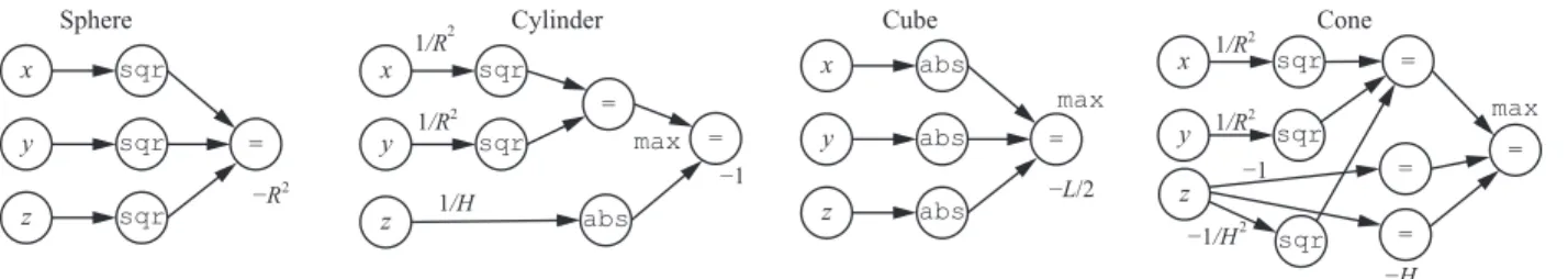
Sphere: F(x, y, z) = x2₊_y2₊_z2₋_R2 Cylinder: F(x, y, z) = maxx2_R+2y2, |z| H −1 Cube: F(x, y, z) = max(|x|,|y|,|z|)− L 2 Cone: F(x, y, z) = max(x2_R+2y2 − z2 H2,−z, z−H) (2.1)

An advantage of implicit surfaces is that the composition of shapes can be easily expressed as the composition of functions, and a composite function can be represented by a (directed acyclic) computation graph, in the same way a neural network is represented as a computation graph.

Suppose a computation graph G = (V, E). It includes a set of nodes V = {x, y, z} ∪ {v1, v2,· · · } ∪ {t}, which includes three input nodes{x, y, z}, a variable number of internal nodes

{v1, v2,· · · }, and a single output nodet. Each nodev ∈ V (excluding input nodes) is associated

with a scalar biasbv, a reduction functionrvthat maps a variable number of real values to a single scalar, and an activation functionφv that maps a real value to a new value. In addition, each edge e∈E is associated with a weightwe.

It is worth noting that different from a standard neural network or a Compositional Pattern Producing Network (CPPN) that only usessumas the reduction function, our reduction function

(28)

x y z sqr sqr sqr = z abs = x y sqr sqr = max 1/R2 1/R2 1/H −1 x y z abs abs abs = max −L/2 _z sqr = x y sqr sqr = 1/R2 1/R2 −1/H2 −1 = −H = max Sphere −R2

Cylinder Cube Cone

Figure 2.2: The computation graphs of four primitive shapes defined in Equation2.1. The unlabeled edge weight and node bias are0, and the unlabeled reduction function issum.

x y z = x’ y’ z’ x y z = −b1 −b2 −b3 (λA)−1

Figure 2.3: Shape transformation represented by graph operation. Left: the graph of the shape before transfor-mation. Right: the graph of the shape after transforma-tion.

can besum,maxormin. As will become clear, this is to allow straightforward composition of shapes.

To evaluate the computation graph, each node takes the weighted activations of its predecessors and applies the reduction function, followed by the activation function plus the bias. Figure2.2 illustrates the graphs of the functions defined in Equation2.1.

Shape transformation To evolve shapes, we define graph operations to generate new shapes from existing ones. We first show how to transform an individual shape. Given an existing shape represented byF(x, y, z), let F(T(x, y, z))represent a transformed shape, whereT : _R3 _→

R3

is a 3D-to-3D map. It is easy to verify thatF(T(x, y, z))represents the transformed shape under

translation, rotation, and scaling if we defineT as

T(x, y, z) = (λA)−1[x, y, z]T−b, (2.2)

where A is a rotation matrix, λ is the scalar, and the b is the translation vector. Note that for

simplicity our definitions have only included a single global scalar, but more flexibility can be easily introduced by allowing different scalars along different axes or an arbitrary invertible matrixA.

(29)

x y z = F1 (1) (1) (1) x y z (2) (2) (2) = F2 x y z = F1 = F2 = min

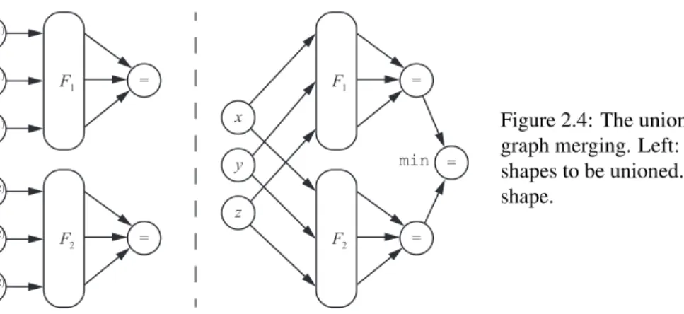
Figure 2.4: The union of two shapes represented by graph merging. Left: the respective graphs of the two shapes to be unioned. Right: the graph of the unioned shape.

in Figure2.3. Given the original graph of the shape, we insert 3 new input nodesx0, y0, z0before the original input nodes, connect new nodes to the original nodes with weights corresponding to the elements of the matrix(λA)−1_{, and set the biases of the original nodes to the vector}₋_b_.

Shape composition In addition to transforming individual shapes, we also define binary oper-ations over two shapes. This allows complex shapes to emerge from the composition of simple ones. Suppose we have two shapes with the implicit representationsF1(x, y, z)andF2(x, y, z). As

a basic fact [117], the union, intersection, and difference of the two can be represented as follows: Funion(x, y, z) = min(F1(x, y, z), F2(x, y, z))

Fintersection(x, y, z) = max(F1(x, y, z), F2(x, y, z))

Fdifference(1,2)(x, y, z) = max(F1(x, y, z),−F2(x, y, z)).

(2.3)

In terms of graph operations, composing two shapes together corresponds to merging two graphs. As illustrated by Figure 2.4, we merge the input nodes of the two graphs and add a new output node that is connected to the two original output nodes. We set the reduction function (max,min, orsum) and the weights of the incoming edges to the new output node according to the specific composition chosen.

(30)

2.3.2 Evolution Algorithm

Our evolution process follows a standard setup. It starts with an initial population ofnshapes:

{s1, s2,· · · , sn}, all of which are primitive shapes described in Equation2.1. Next,mnew shapes ({s0₁, s0₂,· · · , s0_m}) are created from two randomly sampled existing shapes (i.e. two parent shapes).

Specifically, the two parent shapes each undergo a random rotation, a random scaling and a random translation, and are then combined by a random operation chosen from union, intersection and difference to generate a new child shape. Now, the population consists of a total ofn+m(nparent shapes andmchild shapes). Each shape is then evaluated and given a fitness score, based on which n shapes are selected to form the next population. This process is then repeated to evolve more complex shapes.

Having outlined the overall algorithm, we now discuss several specific designs we introduce to make our evolution more efficient and effective.

Fitness propagation Simply evaluating fitness as a function of individual shape is suboptimal in our case. Our shapes are evolved based on composition, and to generate a new shape requires combining existing shapes. If we define fitness strictly on an individual basis, simple shape primitives, which may be useful in producing more complex shapes, can be eliminated during the early rounds of evolution. For example, suppose our goal is to evolve an implicit representation of a target shape. As the population nears the target shape, smaller and simpler cuts and additions are needed to further refine the population. However, if small, simple shapes, which poorly represent the target shape, have been eliminated, such refinement cannot take place.

We introduce fitness propagation to combat this problem. We propagate fitness scores from a child shape to its parents to account for the fact that a parent shape may not have a high fitness in itself, but nonetheless should remain in the population because it can be combined with others to yield good shapes. Suppose in one round of evolution, we evaluate each of thenexisting shapes and mnewly composed shapes and obtainn+mfitness scores{f1,· · · , fn, f10,· · · , f

0

m}. But instead of directly assigning the scores, we propagate themfitness scores of the child shapes back to the

(31)

parent shapes. A parent shapefiis assigned the best fitness score obtained by its children and itself: fi ←max {fj0 :si ∈π(s0j)} ∪ {fi}

, (2.4)

whereπ(s0_j)is the parents of shapes0_j.

Computational resource constraint Because shapes evolve through composition, in the course of evolution the shapes will naturally become more complex and have larger computation graphs. It is easy to verify that the size of the computational graph of a composed shape will at least double in the subsequent population. Thus without any constraint, the average computational cost of a shape will grow exponentially in the number of iterations as the population evolves, quickly depleting available computing resources before useful shapes emerge. To overcome this issue, we impose a resource constraint by capping the growth of the graphs to be linear in the number of rounds of evolution. If the number of nodes of a computation graph exceedsβt, whereβis a hyperparameter andtis time, the graph will be removed from the population and will not be used to construct the next generation of shapes.

Discarding trivial compositions A random composition of two shapes can often result in trivial combinations. For instance, the intersection of shapeAand shapeB may be empty, and the union of two shapes can be the same as one of the parent. We detect and eliminate such cases to prevent them from slowing down the evolution.

Promoting diversity Diversity of the population is important because it prevents the evolution process from overcommitting to a narrow range of directions. If the externally given fitness score is the only criterion for selection, shapes deemed less fit at the moment tend to go extinct quickly, and evolution can get stuck due to a homogenized population. Therefore, we incorporate a diversity constraint into our algorithm: a fixed proportion of the shapes in the population are sampled not based on fitness, but based on the size of their computation graph, with bigger shapes sampled

(32)

proportionally less often.

2.4 Joint Training of Deep Network

The shapes are evolved in conjunction with training a deep network to perform shape-from-shading. The network takes a rendered image as input, and predicts the surface normal at each pixel. To train this network, we render synthetic images and obtain the ground truth normals using the evolved shapes.

The network is trained incrementally with a training set that consists of evolved shapes. LetDi be the training set after theith iteration of the evolution, and letNibe the network at the same time. The training set is initialized to empty before the evolution starts,i.e.D0 =∅, and the network is

initialized with random weights.

In theith evolution iteration, to compute the fitness score of a shapedin the population, we

fine-tune the current networkNi−1 with Di−1 ∪ {d}—the current training set plus the shape in

consideration—to produce a fine-tuned networkN_id₋₁, which is evaluated on a validation set of real images to produce an error metric that is then used to define the fitness score of shaped. After we have evaluated the fitness of every shape in the population, we update the training set with the fittest shaped∗_i,

Di =Di−1∪ {d∗i}, (2.5)

and set theNd∗

i−1 as the current network,

Ni =N_id−∗1. (2.6)

In other words, we maintain a growing training set for the network. In each evolution iteration, for each shape in the population we evaluate what would happen if we add the shape to the training set and continue to train the network with the new training set. This is done for each shape in the population separately, resulting in as many new network instances as there are shapes in the current population. The best shape is then officially added to the training set, and the corresponding

(33)

Target Evolved shapes

t = 50

t = 5 t = 100 t = 200

t = 10 t = 100 t = 200 t = 400

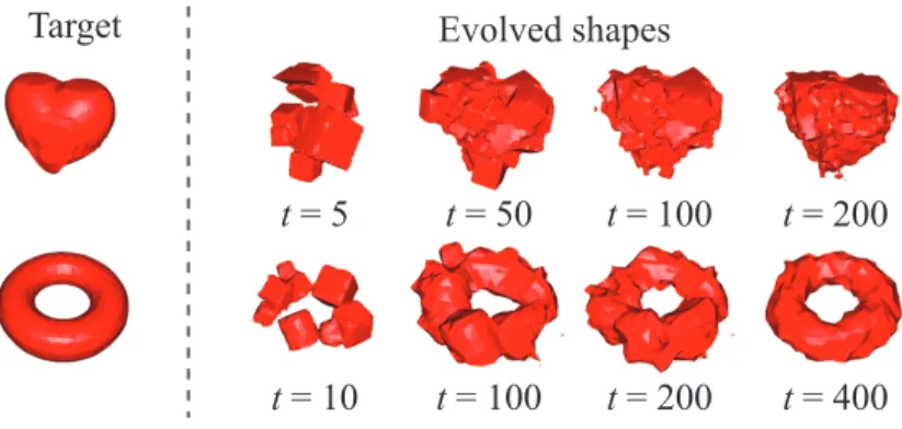
Figure 2.5: Evolution towards a target shape. Left: targets. Right: The fittest shapes in the population as the evolution progresses at different iterations.

fine-tuned network is also kept while the other network instances are discarded. 2.5 Experiments

2.5.1 Standalone Evolution

We first experiment with shape evolution as a standalone module and study the role of several design choices. Similar to [29], we evaluate whether our evolution process is capable of generating shapes close to a given target shape. We define the fitness score of an evolved shape as its intersection over union (IoU) of volume with the target shape.

Implementation details To select the shapes during evolution, half of the population are sampled based on the rankrof their fitness score (from high to low), with the selection probability set to

0.2r_{. The other half of the population are sampled based on the rank}_s_{of their computation graph} size (from small to large), with the relative selection probability set to0.2s_{, in order to maintain} diversity. To compute the volume, we voxelize the shapes to32×32×32grids. The population

sizenis1000and the number of child shapesm = 1000.

Results We use two target shapes, a heart and a torus. Figure2.5shows the two target shapes along with the fittest shape in the population as the evolution progresses. We can see that the evolution is able to produce shapes very close to the targets. Quantitatively, after around 600 iterations, the best IoU of the evolved shapes reaches94.9%for the heart and93.5%for the torus.

(34)

0 25 50 75 100 125 150 175 time / hour 0.00 0.25 0.50 0.75

IoU FitnessProp + DiscardTrivial + Diversity FitnessProp + DiscardTrivial DiscardTrivial ONLY FitnessProp ONLY 0 100 200 300 400 500 600 #iterations 0.00 0.25 0.50 0.75 IoU 0 25 50 75 100 125 150 175 time / hour 0.00 0.25 0.50 0.75

IoU FitnessProp + DiscardTrivial + Diversity FitnessProp + DiscardTrivial DiscardTrivial ONLY FitnessProp ONLY 0 100 200 300 400 500 600 #iterations 0.00 0.25 0.50 0.75 IoU

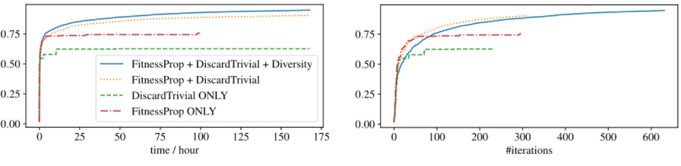
Figure 2.6: The best IoU with the target shape (heart) versus evolution time (top) and the number of iterations (bottom) for different combinations of design choices.

propagation, discarding trivial compositions, and promoting diversity. Figure2.6plots, for different combinations of these choices, the best IoU with the target shape (heart) versus evolution time, in terms of both wall time and the number of iterations. We can see that each of them is beneficial and enabling all three achieves fastest evolution in terms of wall time. Note that, the diversity constraint slows down evolution initially in terms of the number of iterations, but it prevents early saturation and is faster in terms of wall time because of lower computational cost in each iteration.

2.5.2 Joint Evolution and Training

We now evaluate our full algorithm that jointly evolves shapes and trains a deep network. We first describe in detail the setup of our individual components.

Setup of network training We use a stacked hourglass network [102] as our shape-from-shading network. The network consists of a stack of 4 hourglasses, with 16 feature channels for each hourglass and 32 feature channels for the initial layers before the hourglasses. In each round of evolution, we fine-tune the network forτ = 100iterations using RMSprop [150], a batch size of 4,

and the mean angle error as the loss function. Before fine-tuning on the new dataset, we re-initialize the RMSprop optimizer.

Rendering synthetic images To render shapes into synthetic images, we use the Mitsuba ren-derer [60], a physically based photorealistic renren-derer. We run the marching cubes algorithm [85] on the implicit function of a shape with a resolution of64×64×64to generate the triangle mesh for

(35)

rendering. We use a randomly placed orthographic camera, and a directional light with a random direction within 60◦ of the viewing direction to ensure a sufficiently lit shape. All shapes are

rendered with diffuse textureless surfaces, along with self occlusion and shadows. In addition to the images, we also generate ground truth surface normals.

Real images with ground truth For both training and testing, we need a set of real-world images with ground truth of surface normals. For training, we need a validation set of real images to evaluate the fitness of shapes, which is defined as how well they help the performance of a shape-from-shading network on real images. For testing, we need a test set of real images to evaluate the performance of the final network.

We use the MIT-Berkeley Intrinsic Image dataset [8,51] as the source of real images. It includes images of 20 objects captured in a lab setting; each object has two images, one with texture and the other textureless. We use the textureless version of the dataset because our method only evolves shape but not texture. We adopt the official 50-50 train-test split, using the 10 training images as the validation set for fitness evaluation and the 10 test images to evaluate the performance of the final network.

Setup of shape evolution In each iteration of shape evolution, the population size is maintained atn= 100, andm= 100new shapes are composed. To select the shapes, 90% of the population

are sampled by a roulette wheel where the probability of each shape being chosen is proportional to its fitness score. The fitness score is the reciprocal of the mean angle error on the validation set. The remaining 10% are sampled using the diversity promoting strategy, where the shapes are sampled also based on the ranksof their computation graph size (from small to large), with the relative selection probability set to0.5s.

Evaluation protocol To evaluate the shape-from-shading performance of the final network, we use standard metrics proposed by prior work [159,8]. We measure N-MAE and N-MSE,i.e. the

(36)

the mean squared errors of the normal vectors. We also measure the fraction of the pixels whose normals are within 11.25, 22.5, 30 degrees angle distance of the ground-truth normals.

Since our network only accepts 128×128 input size but the images in the MIT-Berkeley dataset

have different sizes, we pad the images and scale them to 128×128 to feed into the network, and

then scale them back and crop to the original sizes for evaluation. 2.5.2.1 Baselines approaches

We compare with a number of baseline approaches including ablated versions of our algorithm. We describe them in detail below.

SIRFS SIRFS [8] is an algorithm with state-of-the-art performance on shape from shading. It is primarily based on optimization and manually designed priors, with a small number of learned parameters. Our method only evolves shapes but not texture, so we compare with SIRFS using the textureless images. Because the published results [8] only textured objects from the MIT-Berkeley Intrinsic Image dataset, we obtained the results on textureless objects using their open source code. Training with ShapeNet We also compare a baseline approach that trains the shape-from-shading network using synthetic images rendered from an external shape dataset. We use a version of ShapeNet [17], a large dataset of 3D CAD models that consists of approximately 51,300 shapes. We evaluate two variants of this approach.

• ShapeNet-vanillaWe train a single deep network on the synthetic images rendered using

shapes in ShapeNet. Both the network structure and the rendering setting are the same as in the evolutionary algorithm. For everyτ RMSprop iterations (the number of iterations used to fine-tune a network in the evolution algorithm), we record the validation performance and save the snapshot of the network. When testing, the snapshot with the best validation performance is used.

(37)

RMSprop training everyτ iterations, initializing from the latest weights. This is because in our evolution algorithm only the network weights are reloaded for incremental training, while the RMSprop training starts from scratch. We include this baseline to eliminate any advantage the restarts might bring in our evolution algorithm.

Ablated versions of our algorithm We consider three ablated versions of our algorithm:

• Ours-no-feedbackThe fitness score is replaced by a random value, while all other parts of the

algorithm remain unchanged. The shapes are still being evolved, and the networks are still being trained, but there is no feedback on how good the shapes are.

• Ours-no-evolutionThe evolution is disabled, which means the population remains to be the

initial set of primitive shapes throughout the whole process. This ablated version is equivalent to training a set of networks on a fixed dataset and picking the one fromn+mnetworks that has the best performance on the validation set everyτ training iterations.

• Ours-no-evolution-plus-ShapeNet The evolution is disabled, and maintain a population of

n+mnetwork instances being trained simultaneously. For eachτ iterations, the network with the best validation performance is selected and copied to replace the entire population. It is equivalent toOurs-no-evolutionexcept that the primitive shapes are replaced by shapes

randomly sampled from ShapeNet each time we render an image. This ablation is to evaluate whether our evolved shapes are better than ShapeNet shapes, controlling for any advantage our training algorithm might have even without any evolution taking place.

2.5.2.2 Results and analysis

Table2.1compares the baselines with our approach. We first see that the deep network trained through shape evolution outperforms the state-of-the-art SIRFS algorithm, without using any external dataset except for the 10 training images in the MIT-Berkeley dataset that are also used by SIRFS.

(38)

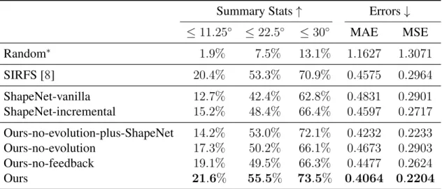
Table 2.1: The results of baselines and our approach on the test images.∗_{Measured by uniformly randomly outputting} unit vectors on the+zhemisphere.

Summary Stats↑ Errors↓

≤11.25◦ ≤22.5◦ ≤30◦ MAE MSE Random∗ ₁_._9% ₇_._5% ₁₃_._1% ₁_.₁₆₂₇ ₁_.₃₀₇₁ SIRFS [8] 20.4% 53.3% 70.9% 0.4575 0.2964 ShapeNet-vanilla 12.7% 42.4% 62.8% 0.4831 0.2901 ShapeNet-incremental 15.2% 48.4% 66.4% 0.4597 0.2717 Ours-no-evolution-plus-ShapeNet 14.2% 53.0% 72.1% 0.4232 0.2233 Ours-no-evolution 17.3% 50.2% 66.1% 0.4673 0.2903 Ours-no-feedback 19.1% 49.5% 66.3% 0.4477 0.2624 Ours 21.6% 55.5% 73.5% 0.4064 0.2204

We also see that our algorithm outperforms all baselines trained on ShapeNet as well as all ablated versions. This shows that our approach can do away with an external shape dataset and generate useful shapes from simple primitives, and the evolved shapes are as useful as shapes from ShapeNet for this shape-from-shading task. Figure2.8shows example shapes at different stages of the evolution, as well as shapes from ShapeNet, and Figure2.7shows qualitative results of our method and SIRFS on the test data.

More specifically, theOurs-no-evolution-plus-ShapeNetablation shows that our evolved shapes

are actually more useful than ShapeNet for the task, although this is not surprising given that the evolution is biased toward being useful. Also it shows that the advantage our method has over using ShapeNet is due to evolution, not idiosyncrasies of our training procedure.

TheOurs-no-evolutionablation shows that our good performance is not a result of well chosen

primitive shapes, and evolution actually generates better shapes. TheOurs-no-feedbackablation

shows that the joint evolution and training is also important—random evolution can produce complex shapes, but without guidance from network training, the shapes are only slightly more useful than the primitives.

(39)

Input PredictionOur Angle Error Angle Error Truth Ground PredictionSIRFS

Figure 2.7: The qualitative results of our method and SIRFS [8] on the test data.

Shape evolution over time

ShapeNet

(40)

CHAPTER 3 Learning to Generate 3D Synthetic Data through Hybrid Gradient

1

3.1 Introduction

Synthetic images rendered by graphics engines have emerged as a promising source of training data for deep networks, especially for vision and robotics tasks that involve perceiving 3D structures from RGB pixels [15,172,155,122,95,164,18,68,140,120,119,175,77]. A major appeal of generating training images from computer graphics is that they have a virtually unlimited supply and come with high-quality 3D ground truth for free.

Despite its great promise, however, using synthetic training images from graphics poses its own challenges. One of them is ensuring that the synthetic training images are useful for real-world tasks, in the sense that they help train a network to perform well on real images. Ensuring this is challenging because a graphics-based generation pipeline requires numerous design decisions, including the selection of 3D shapes, the composition of scene layout, the application of texture, the configuration of lighting, and the placement of the camera. These design decisions can profoundly impact the usefulness of the generated training data, but have largely been made manually by researchers in prior work, potentially leading to suboptimal results.

In this paper, we address the problem of automatically optimizing a generation pipeline of synthetic 3D training data, with the explicit objective of improving the generalization performance of a trained deep network on real images.

One idea is black-box optimization: we try a particular configuration of the pipeline, use the pipeline to generate training images, train a deep network on these images, and evaluate the network

(41)

evaluate Training images

and 3D ground truth

Parameters Performance

3D composition

and rendering train Network weights

Hybrid Gradient Approximate Gradient Analytical Gradient

Real images

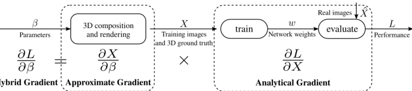
Figure 3.1: Our hybrid gradient method. We parametrize the design decisions as a real vectorβ and optimize the

function of performanceLwith respect toβ. Fromβto the generated training images and ground truth, we compute

the approximate gradient by averaging finite difference approximations. From training samplesXtoL, we compute the

analytical gradient through backpropagation with unrolled training steps.

on a validation set of real images. We can treat the performance of the trained network as a black-box function of the configuration of the generation pipeline, and apply black-black-box optimization techniques. Recent works [171, 123] have explored this exact direction. In Chapter 2, we use genetic algorithms to optimize the 3D shapes used in the generation pipeline. In particular, we start with a collection of simple primitive shapes such as cubes and spheres, and evolve them through mutation and combination into complex shapes, whose fitness is determined by the generalization performance of a trained network. We have shown that the 3D shapes evolved from scratch can provide more useful training data than manually created 3D CAD models. Meanwhile, Ruiz et al. [123] use black box reinforcement learning algorithms to optimize the parameters of a simulator, and shows that their approaches converge to the optimal solution in controlled experiments and can indeed discover good sets of parameters.

The advantage of black-box optimization is that it assumes nothing about the function being opti-mized as long as it can be evaluated. As a result, it can be applied to any existing function, including advanced photorealistic renderers. On the other hand, black-box optimization is computationally expensive—knowing nothing else about the function, it needs many trials to find a reasonable update to the current solution. In contrast, gradient-based optimization can be much more efficient by assuming the availability of the analytical gradient, which can be efficiently computed and directly correspond to good updates to the current solution, but the downside is that the analytical gradient is often unavailable, especially for many advanced photorealistic renderers.