WP 11-07
STEFAN GRUBERUniversity of Innsbruck, Innsbruck, Austria University of Bologna, Bologna, Italy
and
Rimini Centre for Economic Analysis, Rimini, Italy
LUIGI MARATTIN University of Siena, Siena, Italy
“N
O
T
AXATION WITHOUT
I
NFRASTRUCTURE
”
Copyright belongs to the author. Small sections of the text, not exceeding three paragraphs, can be used provided proper acknowledgement is given.
The Rimini Centre for Economic Analysis (RCEA) was established in March 2007. RCEA is a private, non-profit organization dedicated to independent research in Applied and Theoretical Economics and related fields. RCEA organizes seminars and workshops, sponsors a general interest journal The Review of Economic Analysis, and organizes a biennial conference: Small Open Economies in the Globalized World (SOEGW). Scientific work contributed by the RCEA Scholars is published in the RCEA Working Papers series.
The views expressed in this paper are those of the authors. No responsibility for them should be attributed to the Rimini Centre for Economic Analysis.
No Taxation without Infrastructure
Stefan Gruber
a,b,c,∗
, Luigi Marattin
b,daUniversity of Innsbruck, Innsbruck, Austria. bUniversity of Bologna, Bologna, Italy.
cRCEA, The Rimini Center for Economic Analysis, Rimini, Italy. dUniversity of Siena, Siena, Italy.
Abstract
This paper presents a New Economic Geography model with distortionary taxation and endogenized transport costs. Tax revenues finance a public good, infrastructure. We show that the introduction of costly public investment in infrastructure leads to more pronounced agglomeration patterns. With respect to the regions sizes, in the periphery, the price-index for manufacturing goods decreases, whereas for the core, the price-index is rather high since the distortionary effect of taxes dominates. Free riding is beneficial for the periphery, which can devote all its tax revenue to local demand support, generating a positive home market effect and driving the catch-up process.
Key words: New Economic Geography, Taxation, Endogenous Transport Costs, Infrastructure
JEL Classification: F12, H25, H54, R12
∗ Corresponding author. University of Innsbruck, Department of Economics,
Uni-versit¨atsstrasse 15, A-6020 Innsbruck, Austria. Phone: 512-507-7371. Fax: +43-512-507-2980.
Email addresses: [email protected] (Stefan Gruber),
1 Introduction
According to the European Commission, transport infrastructure improve-ments play ’a key role in the efforts to reduce regional and social disparities in the European Union, and in the strengthening of its economic and social co-hesion’ (Commission of the European Communities (1999)). Hence, the Com-mission supports and endorses the development of Trans-European Transport Networks (TEN-T) also 30 axes of priority, which now also encompass the new Eastern European member states, for instance a corridor from Tallin via Riga and Warsaw to Bratislava and Vienna (see Commission of the European Com-munities (2005)). Both the European Union as well as national governments will contribute to its financing. According to Commission of the European Communities (2005), total costs are estimated to be around 330 billion Euros in the period from 2007-2013, where more than half of these costs need to be covered by the member states and other non-EU-related sources. Those TEN-T’s are a key element in the revised ’Lisbon strategy for competitiveness and employment in Europe’, since the EU considers good transport infrastructure, and good accessibility for and of all its members as a key element for economic development in Europe.
The economic literature seems to support this view. According to Limao and Venables (1999), the elasticity of trade volumes with respect to transport costs is estimated at around −2.5, i.e., halving transport costs increases the volume of trade by a factor of five. For outside the EU, Fan and Zhang (2004) in a study on Chinese rural regions confirm that infrastructure is a key to rural development, particularly in all non-agricultural sectors. Henderson et al. (2001) point into a similar direction for African countries and regions.
In this paper we look at the users of infrastructure, firms and consumers, and we explore the links between infrastructure and its (public) financing through taxes. The vehicle being employed in this paper is a simple New Economic Geography (henceforth: NEG) model following Krugman (Krugman, 1991a,b) and Fujita et al. (1999), where we put two things into the focus of research, (i) endogenizing transport cost, and (ii) regional governments and taxation. According to Puga (2002), those models are suitable for this type of analysis, since they focus on the relations between transport costs, agglomeration, and regional disparities, which makes them especially useful for studying to study the role of (transport) infrastructure.
The endogenization of transport costs comes in two steps. First, introducing a corporate sales tax generates revenues for the regions. Regional governments allocate these tax revenues between infrastructure investments and lump-sum transfers to their respective region’s population. Second, the infrastructure is being built using the same production technology as for the manufactured good. The quantity of infrastructure provided is weighted by a scaling and efficiency parameter which determines the amount by which the transport costs are being reduced. These reduced transport costs, of course, influence the firms’ decisions on location and trade.
In the literature on NEG and international trade, there have been a lot of theoretical and empirical contributions investigating public finance, taxation-related problems and, on the other hand, transport costs. As to the former, the literature dates back to the basic tax competition model (for an excellent survey, see Wilson (1999) and Krogstrup (2002)). More recent contributions include Andersson and Forslid (2003) who build a NEG-model where the tax revenue collected is used to finance a public good entering the utility function.
They use the analytically solvable model of Forslid and Ottaviano (2003) and analyze how the tax competition game between countries affects the distribu-tion of workers; they find that even perfectly coordinated tax increases across countries destabilize the dispersion equilibrium of workers.
Baldwin and Krugman (2004) focus on international tax competition and start from the observation that in the European integration process a downward levelling of tax rates has not been observable so far, but there is rather a gradual increase in taxation as the integration process moves on. Similarly to Puga’s bell-shaped agglomeration pattern (see Puga, 1999) which emerges during integration (i.e. disparities between regions first become large, then diminish), Baldwin and Krugman (2004) find the same for tax rates. By using a simple two-region NEG-model in which governments collect taxes from firms’ profits, they challenge the result of the standard tax-competition literature predicting a race to the bottom in tax rates in order to attract firms. They insert agglomeration issues to explain the dynamics of industrial integration and tax rates in Europe.
As for the literature on transport costs, the way they are usually being mod-elled is the ”iceberg” assumption, formally introduced by Samuelson (1952, 1954), even though the first formulation dates back to Von Th¨unen (1826). Bottazzi and Ottaviano (1996) present an overview of various attempts to deal with transport costs in international trade, and provide a general model to evaluate iceberg transport costs, and other alternatives of modelling trans-portation in international trade.
Anderson and van Wincoop (2004) provide a theoretical and empirical analysis of all costs involved in shipping a good from the producer to the final consumer,
also addressing some important measurement issues. Duranton and Storper (2005) start from the empirical observation of declining transport costs, and propose a model of vertically linked industries in which providing a given level of quality to suppliers becomes more costly with distance. Their conclusion is that, due to the fact that lower transport costs imply that higher quality inputs are traded in equilibrium, trade costs can increase despite lower transport costs.
Larch (2005) introduces a model of international trade with multinational en-terprises with a separate and multinationalized transport sector. This allows, for instance, to relax the assumption that transport costs are the same for all goods, and to disentangle the production of goods and transport services. However, there are still exogenously given transport costs for shipping goods. Kilkenny (1998) deals with transport costs in a general equilibrium model us-ing a bilateral regional Social Accountus-ing Matrix, specifically aimed at rural development issues. She shows the existence of an initially negative, but ulti-mately positive relationship between a reduction of transport costs and rural development. The basic intuition is that reducing transport costs from rural locations may also reduces transport costs to rural areas.
However, in all these contributions, transport costs are still exogenously given. Our contribution looks at regional governments who collect distortionary taxes via a corporate sales tax, so to finance investment in public infrastructure, which in turn decrease transport costs. It can be shown that public infrastruc-ture investments lead to more pronounced agglomeration patterns, i.e. the concentration of industries is fostered, which confirms previous results by An-dersson and Forslid (2003) or Baldwin et al. (2003). Nonetheless, this is also
beneficial for the region ending up as the periphery, since also in this region the price index for manufactured goods decreases, which is due to cheaper im-ported product varieties. The reduction of transport costs is very effective for high initial values of trade costs (i.e. before infrastructure investments), while there are less absolute effects when transport costs are already low. In terms of regional policy, it can be shown that it might be useful if such infrastructure investments are only financed by the central region (i.e., the periphery receiv-ing for instance structural funds benefits by the EU, or - in terms of modelreceiv-ing - being a free rider in infrastructure provision), since both regions benefit from such investments, while the periphery can spend its locally collected taxes for local purposes.
The remainder of the paper is organized as follows: Section 2 introduces the model, Section 3 briefly lines out the analyses being conducted. Section 4 investigates the core-periphery patterns, as well as the effects of the infras-tructure provided on trade costs and firms, whereas Section 5 looks at the sensitivity of the model and provides additional insights regarding the major policy parameters. The last Section summarizes and concludes.
2 The Model
2.1 Households
There are two regions, referred to as region 1 and 2, and indexed as {i, j} =
{1,2}. Both regions produce two goods, X andZ.Z is a homogenous agricul-tural good produced at constant returns to scale by a competitive industry.X -goods (manufacturing -goods) are differentiated in the usual Dixit and Stiglitz
(1977) fashion. Firms may sell on the local market and export to the other region, where the number of firms from region i is denoted by ni. Therefore,
Xij are the exports of region i-based firms to region j1. Xic denotes the
con-sumption of X in region i, being a CES aggregate of the individual varieties. The utility of regioni (Ui) can thus be formulated as follows:
Ui=Xicµ(Zii+Zji)1−µ, Xic≡ ni(Xii)σ−σ1 +n j µ X ji 1 +τ ¶σ−1 σ σ σ−1 , (1)
whereµ denotes the Cobb-Douglas expenditure share for differentiated prod-ucts, and σ >1 is the elasticity of substitution between varieties.
We assume that Z-goods are costlessly tradable across regions, whereas X -goods trade incurs iceberg transport costs (τ), which are symmetric for either direction of shipment. In terms of quantity, one unit of consumption of an
X-variety in region j requires a firm in i to send (1 +τ) units. For conve-nience, quantities of X are defined as firm-specific productions for the re-spective foreign market. However, as in our model transport costs may vary with government expenditures (as outlined below), the transport costs are not exogenously given in this setting.
As usual, the consumer’s maximization problem can be solved in two steps. In the first step, each variety Xji needs to be chosen such that it minimizes the
cost of attaining Xic, whatever the consumption ofXic is. In the second step,
consumers allocate income between the Z-good, and the composite X-good. Letpji be the price of anX-variety in regioniproduced by a firm in region j.
The price for the homogenous agricultural good, qi, is indexed once, since all
must face the same price qi. We takeq1 as the num´eraire. Further,Pi denotes
the price aggregator, defined as the minimum cost of buying one unit ofXi at
prices pji of an individual variety:
Pi = min Xji
X
i,j
pjiXji s.t. Xi = 1. (2)
The first-stage budgeting problem leads to:
Xji= (pji)−σPiσ−1αYi ∀ i, j ∈ {1,2}, (3)
where Yi denotes total expenditures of consumers in region i. Identical price
elasticities of demand and identical marginal costs (technologies) within a re-gion ensure that the price of a locally produced manufacturing good is equal to the mill price for exports. Hence, prices of all manufacturing goods produced in one region are equal in equilibrium.pi denotes the price of all goods produced
in region i. With these assumptions, the price aggregatorPi of differentiated
goods consumed in region i can be written as
Pi = h nip1i−σ+nj((1 +τ)pj)1−σ i 1 1−σ . (4)
Note that due to the adopted assumptions about technology, factor markets, and demand − in equilibrium− pi ≡pii =pji and pj(1 +τ)≡ pji =pii. The
second-stage budgeting yields the division of expenditures between the two sectors: Xic= µ Pi Yi, (5) Zii+Zji= 1−µ qi Yi (6)
2.2 Factor Markets, Production and Income
Let wLi and wT i denote the nominal factor rewards of labor and land in
re-gioni, respectively. There is perfect competition in theZ-sector, and each firm produces under constant returns to scale using a CES production technology, employing labor (L) and land (T) (where ’b’ is the coefficient forT and ’1−b’ for L), with an elasticity of substitution of 1/(1−ρz) and (−∞ < ρz < 1).
As all firms face the same factor prices and the CES technology is homo-thetic and exhibits constant returns to scale, [(1−b)Lρz
i +bTiρz]
1
ρz, all firms in a region face the same unit input coefficients. The region specific unit in-put coefficients for the two factors of Z-production can be derived by cost minimization subject to this CES technology:
aLzi= µ w Li 1−b ¶ 1 ρz−1 Ã wρz T i b ! 1 ρz−1 + Ã wρz Li 1−b ! 1 ρz−1 −1 ρz (7) aT zi= µw T i b ¶ 1 ρz−1 Ã wρz T i b ! 1 ρz−1 + Ã wρz Li 1−b ! 1 ρz−1 −1 ρz , (8)
Variable unit costs (i.e., marginal costs)cZi satisfy
cZi≥aLziwLi+aT ziwT i ⊥ Zii ≥0, (9)
where⊥indicates that at least one of the adjacent conditions has to hold with equality. This implies
cZi≥qj ⊥ Zij ≥0. (10)
There is monopolistic competition in the X-sector, and again each firm pro-duces under a CES production technology, using labor (L) and land (T) (where
’a’ is the coefficient for L and ’1−a’ for T), with an elasticity of substitu-tion of 1/(1−ρx) and (−∞ < ρx < 1). As all firms face the same factor
prices and the CES technology is homothetic and exhibits constant returns to scale, [aLρx
i + (1−a)Tiρx]
1
ρx, all firms in a region face the same unit in-put coefficients. The region specific unit inin-put coefficients for the two factors of X-production can be derived by cost minimization subject to this CES technology: aLxi= µw Li a ¶ 1 ρx−1 Ã wρx Li a ! 1 ρx−1 + Ã wρx T i 1−a ! 1 ρx−1 −1 ρx (11) aT xi= µ w T i 1−a ¶ 1 ρx−1 Ã wρx Li a ! 1 ρx−1 + Ã wρx T i 1−a ! 1 ρx−1 −1 ρx (12)
Additionally, X-sector firms require labor (aLni) and land to set up plants
(aT ni), leading to increasing returns to scale in production.
Factor market clearing in region i for labor (Li) and land (Ti) requires
Li≥aLxini(Xii+Xij) +aLnini+aLxiIi+
aLziwLi(Zii+Zij) ⊥ wLi ≥0, (13)
Ti≥aT xini(Xii+Xij) +aT nini+aT xiIi+
aT ziwT i(Zii+Zij) ⊥ wT i ≥0, (14)
where Ii denotes the infrastructure provided in region i.
Variable unit costs of producing an X-variety in region i are given by cXi =
aLxiwLi+aT xiwT i. There is a fixed markup over variable costs, which is
de-termined by the elasticity of substitution between varieties. Given that under CES-utility demand for all varieties is positive, the price setting behavior by
firms is given by pi =cXi σ σ−1 1 1−taxi , (15)
wheretaxi represents the tax rate imposed on firms profits in order to finance
public infrastructure provision, which will be laid out in the next subsection. Free entry implies that firms earn zero profits, since operating profits are used to cover fixed costs. The corresponding zero profit condition determines the numbers of firms.
Manufacturing firms in ihave to bear fixed costs ofF Cni=aLiwLi+aT niwT i.
The zero profit condition, therefore, implies
F Cni ≥
pi(Xii+Xij)
σ (1−taxi) ⊥ ni ≥0. (16)
All factors are owned by the households, so that consumer income (i.e., GNP) in region i is given by
Yi =wLiLi+wT iTi+ (1−κi)Gi (17)
The equivalence of total factor income (Yi, Yj) and demand in each region
implicitly balances payments between regions.
Real factor rewards (ω) are normalized by region-specific costs of living,
Pi−µqµi−1, and are thus given by:
2.3 Taxation, Infrastructure, and Transport Costs
In our model we aim at endogenizing transport cost by tax-financed and pub-licly provided infrastructure.
Taxes (taxi) are introduced as a distortionary sales tax. The profit function
of firms therefore becomes
Πi =pi(Xii+Xij) (1−taxi)−cXi(Xii+Xij)−F Cni, (19)
where Πi are the profits of a regioni firm.
The distortionary effect of this tax can be seen in the resulting pricing equation (replicating equation 15): pi =cXi σ σ−1 1 1−taxi (20)
Hence, the total tax revenues, and subsequently total government spending in region iis
Gi =taxipini(Xii+Xij) +T Ri, (21)
where T Ri are transfers by other administrative bodies to region i’s
govern-ment, such as contributions by the European Commission’s structural funds to regional development policy measures. These transfers are exogenous to the model, i.e. public spending in region i can be higher than its actual budget without incurring a deficit.
From these tax revenues, a fraction 0 < κi < 1 is devoted to infrastructure
regioni’s population. For simplicity, we assume that the production technology for infrastructure is the same as for manufacturing goods, but without being subject to economies of scale. Thus, the amount of infrastructure (Ii) being
provided by region i’s government is
Ii =
κiGi
aLxiwLi+aT xiwT i
. (22)
We assume that both regions’ infrastructure contributes to the reduction of transport costs for shipments between the two regions. Hence, the resulting endogenously determined value for transport costs is determined by
τ = ti
(Ii+Ij + 1)β
, (23)
where ti is an ’initial value’ for transport costs, which also corresponds to a
’no-tax scenario’ without taxes and infrastructure, i.e. to the standard NEG-model with exogenously given transport costs. It may also be regarded as general impediments to trade between the two regions. 0< β <1 is a scaling parameter which also reflects the ’effectiveness’ of the infrastructure provided. Furthermore, note that both regions’ infrastructure investments simultane-ously affect the actual reduction of trade costs (τ).
3 Analyzing the Model
The analysis of the model is conducted along several lines of investigation. First, the standard agglomeration structure will be evaluated, which means for this model, that the ’initial value’ of transport costs, i.e. the value oftthat would apply for a scenario without taxes, varies from 1% to 99% of the price of X-goods. Since publicly provided and tax-financed infrastructure might be
interpretable as quite many different things, not just, say, better roads re-ducing travel time, and hence physical transport costs between places, we suggest to interpret the endogenous transport costs (τ) of the present model more generally as trade costs. This is especially important in our model, since regional public authorities usually do not have the opportunity to influence ’pure’ transport costs, but they rather can try to generally improve their re-gion’s competitive position. Secondly, we look at variations of the parameters which are of our primary interest, the tax rate (tax), and the fraction of gov-ernment expenditures devoted to infrastructure building (κ). This also serves to analyze the model’s sensitivity to parameter changes. Thus, the main focus of the following analyses is put on investigating how the parameters which may be influenced by policy makers shape the economy.
In contrast to the standard NEG-models `a la Krugman (1991b), production of the manufacturing good uses two input factors (L and T). In those models it is straightforward to assume that the factor used in the manufacturing sector is mobile across regions. In line with the literature, all factors are immobile in the short run. In the long run, we investigate situations where L is mobile across regions. We have chosen the following parameter values for all of the following simulations: σ= 4, µ= 0.35, β = 0.1, a=b = 0.8, ρx =ρz =−0.5,
L=L1 +L2 = 60, T =T1+T2 = 100, t= 0.7 if constant, taxi = taxj = 0.2
if constant, κi =κj = 1 if constant.
4 Core-Periphery Patterns, Firms, and Trade Costs
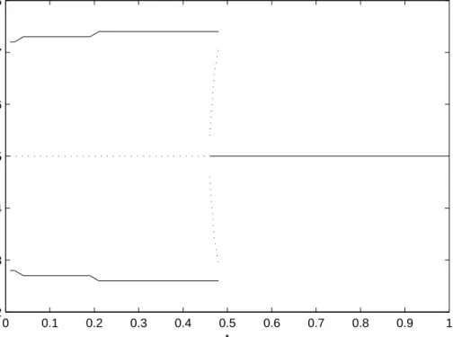
In Figure 1 we show the no-tax and no-infrastructure bifurcation diagram. This is obtained by setting both the tax rates and, therefore, the
infrastruc-ture expendiinfrastruc-tures equal to zero, and varying the initial impediments to trade (t) between 1% and 99% of the price of manufacturing goods, which gives the usual bifurcation diagrams2. The results show that the main qualitative
results from Krugman (1991b) can be replicated, i.e., there is agglomeration at low trade costs, and dispersion at higher trade costs. Due to our produc-tion technology assumpproduc-tions (CES producproduc-tion funcproduc-tion in both sectors, and flexible input coefficients) there is no full-agglomeration equilibrium. However, there is still partial agglomeration at lower initial values of trade costs, and a symmetric equilibrium at higher values of t. Then, in Figure 2 we activate taxes and infrastructure spending by setting the tax rates in both region to
taxi = 0.2 and κi = 13. The endogenization of trade costs through public
infrastructure investments leads the partially agglomerated equilibrium to be sustainable for a larger range of trade costs. The endogenization of trade costs through public infrastructure investments in this framework leads the partially agglomerated equilibrium to be sustainable for a larger range of trade costs. The infrastructure provided by the regions’ governments allows the agglom-erated equilibrium to remain stable for higher initial (i.e., no-tax) values of trade costs. This result confirms Baldwin et al. (2003, Ch. 17), who find that infrastructure which facilitates interregional trade leads to increased spatial concentration. Baldwin et al. (2003, Ch. 17) also note that this subsequently leads to higher growth in the whole economy (i.e., also in the periphery), and to a decrease in nominal income inequalities between the center and the periphery.
− Figures 1 and 2 −
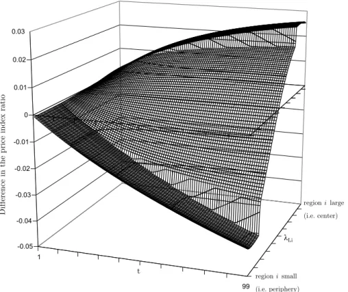
Lower trade costs due to public infrastructure investments also influence re-gional disparities. The price index of manufacturing goods decreases as trade
costs diminish. This effect is the net result of two opposing forces, (i) lower trade costs leading to lower costs for imported goods, hence constituting a positive price index effect, and (ii) more goods need to be imported since some firms might have an incentive to relocate to the center, which in turn means that more goods have to be imported in total, resulting in a negative price index effect.
Comparing the differences of the price indices for manufacturing goods in the benchmark case to the no-tax (and hence no-infrastructure) scenario, it turns out that the differences in price index ratios is high at high trade costs, and approach zero as trade costs approach zero. As a result, public infrastruc-ture provision by regional authorities is beneficial for the center as well as the periphery, since the prices for manufacturing goods also decrease in the periphery despite hosting less firms as trade costs diminish (for the latter, see also Figure 7, left panel). Looking at Figure 3, it can be seen that at low values of t, the are almost no differences in the price indices between the small (peripheral) and the large (central) region. At higher t’s, the smaller region’s price index decreases compared to the no-infrastructure setting, since infrastructure reduces transport costs, and hence the price of imported goods. The larger region does not enjoy these benefits since it host already the major share of firms. Therefore, infrastructure investments do not play an important role, but instead the larger region suffers from the taxes imposed. This result confirms Kilkenny (1998) who finds that a reduction of transport costs in rural areas leads to an improvement in rural development.
Looking at the amount of tax revenues, which subsequently become govern-ment expenditures, we find a Laffer-curve shape as the size of a region varies. The maximum tax revenues are reached when a region hosts around 75% of the workers, depending on the value oft(see Figure 4). Note that this corresponds to the size of the larger region in the partially agglomerated equilibrium of Figure 2.
− Figure 4 −
Changes in the exogenously given tax rate (tax) cause the agglomeration equi-librium to be sustainable for a larger range of values oftthan in the benchmark case, provided that the tax rate does not become too high. Quite similar effects are observable when altering the fraction of government expenditures devoted to infrastructure provision (κ). The higher κ, the more sustainable agglom-eration becomes due to the fact that more (or better) infrastructure will be provided. But also a κi =κj = 0 does not lead to a symmetric agglomeration
equilibrium only. Of course, in this case no infrastructure can be provided to reduce trade costs, but at lower initial values of t a core-periphery structure emerges in this case, too.
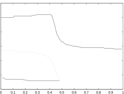
If one region free rides in infrastructure provision, i.e. κi = 0 while κj >0, a
somewhat different picture develops (see Figure 5). In this situation, there is again partial agglomeration at low trade costs. However, the smaller region’s equilibrium breaks as the initial trade costs approach about t= 0.5, while the (at lowt’s) larger region’s equilibrium agglomeration path remains sustainable over the whole range of trade costs.
Note that as the smaller region’s equilibrium breaks, the larger region’s ag-glomeration becomes significantly less pronounced. This equilibrium becomes
the only one at higher trade costs, and decreases even slightly belowλLi = 0.5.
This means that at higher initial trade costs, there emerges a picture which is similar to the original core-periphery pattern, but slightly asymmetric. How-ever, the asymmetry is not as pronounced as one might have expected it. The free riding region is almost of equal size as the other one (λLi ≈ 0.48). This
is due to the fact that there is no interregional tax competition in the present setup, and that the region which free rides in infrastructure provision trans-fers its entire tax revenues lump-sum to its population generating additional income and hence additional demand. Therefore, there are always some firms having incentives to locate in the free riding region.
Looking at this result from a social planner’s perspective, we find that free rid-ing for a smaller, or a peripheral region is beneficial. A region which should be better connected to central regions by implementing regional policy measures, therefore, should not contribute to public infrastructure investments if initially the trade costs are high (i.e., before implementing any policy measures). This is due to the fact that the free riding region keeps their tax revenues within the region and generates additional income through the lump-sum redistribution of the tax revenues among its population. A better infrastructure, although financed by a different region, develops the connections between those regions such that it becomes possible, also for the more remotely located region, to attract additional firms. Note, that instead of tax competition, the role of com-petition in this model is played by the independent decision of each regional government to set itsκ, i.e. to divide its government expenditures between in-frastructure investment and lump-sum transfers to its respective population.
Asymmetric taxation between the two regions exclusively leads to agglomer-ation in the region with the lower tax rate (region j in this case). This is a quite intuitive a result since the region with a lower tax rate attracts more firms which in turn attract more workers (see Figure 6). Note that region i
always remains small in this scenario (it is the only stable equilibrium), while region j is rather big.
− Figure 6 −
A similar result, though through a different channel, occurs when the endow-ment with land (T) differs across region. In this case, there is agglomeration in the region endowed with more land. This is due to the fact that both goods,
X and Z, require someT in production and X-sector firms also need land as a fixed input for setting up their production plant. Only at very low initial trade costs, agglomeration in the smaller region (in terms of T) may be a long run stable equilibrium.
Varying the scaling and efficiency parameter β shows that a higher β leads (i) to a more significant reduction in trade costs (τ) which in turn makes (ii) the partially agglomerated equilibrium more sustainable, also at higher initial values of trade costs (t).
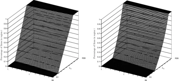
Looking at regioni’s share of firms and at the infrastructure provided in region
i, we note several things. First, if region i has less than about 20% of the world’s endowment with labor (see theλLi-axis in Figures 7 and 8, left panel
in each case), there are no firms headquartered in regioni(Figure 7), and thus there is also no infrastructure being provided by regioni (Figure 8). The two right hand panels of these two figures show the same analyses for asymmetric taxation (taxi = 0.5, while taxj remains at its original value of 0.2). Figure 7
shows that due to the higher tax rate in region i, the area without any firms in region i increases by about 50%, and hence also the area where region i is not able to provide public infrastructure4. From Figure 6 we know that the
only stable equilibrium configuration for workers emerges when regionihosts about 25% of the workers (in region j there are the remaining about 75%). Hence, in this asymmetric taxation-scenario, only the region with lower taxes (i.e., region j) will host firms (for all values of t or τ). Thus, region i needs to import all of its manufacturing goods from region j. This constitutes the same result as a full-agglomeration equilibrium of a standard model, despite regioni hosting some of the workers in our scenario. The tax-rate-differential (of 30%) between both regions outweighs the rather large share of workers in regioni. Looking at the right panel of Figure 7, if regioniwas very large (i.e., at a large λLi), firms would have an incentive to relocate to j because of the
lower tax rate there, until the stable equilibrium is reached.
− Figures 7 and 8 −
Turning to the endogenized trade costs (τ), and investigating the influence of public infrastructure provision on the reduction of trade costs, we generally find the following. The higher the initial trade costs are, the larger the absolute effect of infrastructure, and thus the larger the reduction of trade costs will be. Hence, the absolute decrease of trade costs caused by infrastructure in-vestments is higher if the initial impediments to trade are high. This decrease would be even stronger if the scaling and efficiency parameter β was higher, also at higher tax rates. In other words, for regions being rather remote from economic centers and having high interregional impediments to trade, it makes more sense to strengthen the infrastructure network than for quite integrated or centrally located regions where trade costs are already quite low.
Some of the above findings can easily be seen by inspecting the equations on infrastructure provision, equations 21, 22, and 23. Plugging equation 21 into 22, we obtain
Ii =
κi[taxipini(Xii+Xij) +T Ri]
aLxiwLi+aT xiwT i
, (24)
and plugging the resulting equation 24 into 23 we have
τ = h ti κi[taxipini(Xii+Xij)+T Ri] aLxiwLi+aT xiwT i + κj[taxjpjnj(Xjj+Xji)+T Rj] aLxjwLj+aT xjwT j + 1 iβ, (25)
Inspecting equation 24, public infrastructure investments are generally facili-tated by higher taxes (since there is more money to be spent), a larger number of firms and higher quantities being produced in a region (more firms pro-ducing higher quantities pay more taxes). Consequently, this leads to larger reductions of trade costs (see equation 25). Additionally, a higher efficiency of the infrastructure provided (i.e., a higher β), also leads to a stronger re-duction of trade costs. Similarly, some external funding via transfer payments (where ’external’ means external to regional budgets, denoted by T R in the above equations) facilitates and increases regional public infrastructure pro-vision. Clearly, infrastructure becomes more expensive, and thus its provision decreases, as the factor prices and/or the factor input requirements rise.
5 Sensitivity Analysis
The sensitivity of the model can be analyzed in several ways, which also pro-vides additional insights. Apart from doing the fairly standard simulation exercise of varying transport costs (which in this paper means varying the
initial impediments to trade, t), we also simulate variations of the two policy parameterstaxandκ. We call these two parameters ’policy parameters’, since these two values may be chosen by the regional decision makers. Additionally, various t’s for these two scenarios are being tested.
5.1 Variations of µ, σ and ρ
Variations of the elasticity of substitution between varieties of the differenti-ated manufacturing good, σ, and the technical rate of substitution between input factors,ρ, show that the model’s reactions are very stable. In terms of the bifurcation diagrams, this means that they are either stretched or compressed (i.e., more or less pronounced agglomeration equilibria) or shifted to the left or to the right (i.e., more or less sustainable agglomeration or dispersion equilib-ria) as it has to be expected qualitatively by the respective parameter change. The same applies for the income expenditure share for manufactures,µ, where a higher µ leads to stronger agglomerations in equilibrium.
5.2 Variations of the tax rate and the government expenditures for infras-tructure
Varying the tax rate (tax) and the fraction of government expenditures de-voted to infrastructure building (κ) shows no effect as the initial trade costs are high (t= 0.7). We have first chosen a rather high value oftfor the analyses, in order to be able to reflect the situation that may occur between centrally and peripherally located regions. As all the bifurcation diagrams from before show, there is always a stable symmetric equilibrium only at these values of
t. Hence, variations of tax and κ only affect more integrated economies with lower trade costs.
Att = 0.2, the opposite picture develops. Here, agglomeration is a sustainable equilibrium for all values of both tax and κ, since trade costs are simply low enough to render agglomeration sustainable, no matter how the other parameters are configured.
As the fraction of government expenditures devoted to infrastructure invest-ments, κ, varies from 0 to 1, interesting insights may be gained as far as the development of trade costs (τ) is concerned. Figure 9 (left panel) shows that an equal division of the government expenditures between infrastructure in-vestments and transfers to the population (i.e. κ = 0.5) leads to a reduction of trade costs by about 0.09. An additional increase of κ up to κ= 1 reduces trade costs only by a further 0.03 points. Thus, a region’s government needs to account for this decreasing utility of infrastructure investments when de-ciding on its policy measures. The right panel of Figure 9 shows that a higher efficiency of infrastructure provision (β) increases the reduction of trade costs, while the decreasing utility of infrastructure investments remains evident.
− Figure 9 −
Variations of the tax rate do not show any significant changes in the core-periphery patterns as long as they are coordinated in both regions. Also, the development of tax revenues and infrastructure provision is unaffected by co-ordinated changes in the tax rate. However, the effects on trade costs are noteworthy. No matter what the tax rate is, trade costs are lowest when work-ers (and industries) are concentrated in either of the regions, whereas they tend to be somewhat higher when the regions are of equal size (see Figure 10).
−Figure 10 −
6 Conclusions
In this paper we endogenize transport (trade) costs using the basic New Eco-nomic Geography model, in which we also enrich the production side by al-lowing two factors of production. The endogenization of transport costs comes in two steps. First, introducing a corporate sales tax generates revenues for the regions. Regional governments allocate these tax revenues between in-frastructure investments and a lump-sum transfer to their respective region’s population. Second, the infrastructure is being built using the same production technology as for the manufactured good. The quantity of infrastructure pro-vided is weighted by a scaling and efficiency parameter determines the amount by which the transport costs are being reduced. These reduced transport costs enter into the model influencing the firms’ decisions on location and trade. Our results can be summarized as follows. First, confirming the previous re-sults from Andersson and Forslid (2003) or Baldwin et al. (2003), although in different settings, we show that the introduction of costly public invest-ment in infrastructure leads to more pronounced agglomeration patterns: the core-periphery pattern becomes more sustainable for a wider range of initial trade costs. Varying the tax rate (or the fraction of public revenue devoted to infrastructure) renders the agglomeration equilibrium even more sustainable, provided that the tax rate does not become too high. The stability of core-periphery equilibrium is further supported by the finding according to which public revenue is maximized when one of the region hosts approximately 75% of the manufacturing industries.
Second, the effects on prices are the following. With respect to the regions sizes, for the region ending up as periphery, generally the price-index for man-ufacturing goods decreases, since the import-price-effect prevails on the nega-tive price-index effects. For the region ending up as the core, the price-index is rather high since the distortionary effect of increased taxation (used to finance infrastructure) dominates. With respect to initial trade cost, we find that as they approach zero, the price-index with infrastructure spending approaches the value of the same index without infrastructure spending. As trade costs in-crease, the former decreases, thereby displaying the beneficial effects of public investment.
Third, free riding is beneficial. We show that having infrastructure being fi-nanced only by the larger region makes its equilibrium agglomeration path sustainable over the whole range of initial trade costs. Furthermore, the pe-riphery can devote all its tax revenue to local demand support, thereby gen-erating additional income and a positive home market effect (which actually ends up driving the catch-up process).
Finally, decreasing marginal utility of infrastructure spending, and the im-portance of the efficiency parameter, strengthen the conclusion that at high initial trade costs it is socially desirable to increase taxation (especially in the larger region) in order to finance public investment.
However, our framework lacks interregional tax competition, and the strategic interactions between core and periphery regarding infrastructure building. We feel that in this direction, enriched by public finance considerations about different types of taxation on different agents, some promising analysis can be carried out in the future.
Acknowledgements
We would like to thank Antonio Accetturo, Marius Br¨ulhart, Simon Loretz, Jim Markusen, Giordano Mion, Gianmarco Ottaviano, Michael Pfaffermayr, and participants at the 2006 ETSG Meetings in Vienna as well as at the 2007 Workshop on Economic Geography at the Rimini Center for Economic Analysis for valuable comments and discussions. Of course, all the remaining errors are ours.
We gratefully acknowledge financial support from the TERA project funded by the European Commission within the 6th Framework Programme of RTD
(grant no. FP6-SSP-2005-006469). This publication does not necessarily re-flect the European Commission’s views and in no ways anticipates the Com-mission’s future policy in this area.
Notes
1Whenever we use iandj from the set{1,2}, this implies that i6=j.
2In all the bifurcation diagrams, solid lines denote long-run stable equilibria,
whereas dotted lines depict unstable equilibria.
3Figure 2 constitutes the benchmark case for all the subsequent analyses and
comparisons.
4Note that in those cases where the share of firms in region i is zero and no
infrastructure is being provided, also the tax revenues and hence government ex-penditures are zero.
References
Andersson, F. and R. Forslid, 2003, Tax Competition and Economic Geogra-phy, Journal of Public Economic Theory 5, 279-303.
Anderson, J.E. and E. van Wincoop, 2004, Trade Costs, NBER Working Paper 10480.
Baldwin, R.E., Forslid, R., Martin, P., Ottaviano, G.I.P., and F. Robert-Nicoud, 2003, Economic Geography and Public Policy (Princeton University Press, Princeton).
Baldwin, R.E. and P. Krugman, 2004, Agglomeration, Integration, and Tax Harmonization, European Economic Review 48, 1-23.
Borck, R. and M. Pfl¨uger, 2006, Agglomeration and Tax Competition, Euro-pean Economic Review 50, 647-668.
Bottazzi, L. and G.I.P. Ottaviano, 1996, Modelling Transport Costs in In-ternational Trade: A Comparison among Alternative Approaches, Working Paper no. 105, Innocenzo Gasparin Institute for Economic Research. Commission of the European Communities, 1999, Communication from the
Commission to the Council, the European Parliament, the Economic and Social Committee and the Committee of the Regions on Cohesion and Transport, COM (1998) 806 (Commission of the European Communities, Brussels).
European Commission, Energy and Transport DG, 2005, Trans-European Transport Network, TEN-T, Priority Axes and Projects 2005 (Commission of the European Communities, Brussels).
Dixit, A.K. and J.E. Stiglitz, 1977, Monopolistic Competition and Optimum Product Diversity, American Economic Review 67, 297-308.
Trade with Endogenous Transaction Costs, CEPR Discussion Paper 4933. Fan, S. and X. Zhang, 2004, Infrastructure and Regional Economic
Develop-ment in China, China Economic Review 15, 203-214.
Forslid, R. and G.I.P. Ottaviano, 2003, An Analytically Solvable Core-Periphery Model, Journal of Economic Geography 3, 229-240.
Fujita, M., Krugman, P. and A.J. Venables, 1999, The Spatial Economy -Cities, Regions, and International Trade (The MIT Press, Cambridge, MA). Fujita, M. and J.-F. Thisse, 2002, Economics of Agglomeration (Cambridge
University Press, Cambridge, MA).
Henderson, J.V., Shalizi, Z. and A.J. Venables, 2001, Geography and Devel-opment, Journal of Economic Geography 1, 81-105.
Kilkenny, M., 1998, Transport Costs and Rural Development, Journal of Re-gional Science 38, 293-312.
Krogstrup, S., 2002, What do Theories of Tax Competition Predict for Cap-ital Taxes in EU countries? A Review of the Tax Competition Literature, mimeo., (Geneva, HEI).
Krugman, P., 1991a, Geography and Trade (Leuven University Press and Cambridge University Press, Leuven, Cambridge).
Krugman, P., 1991b, Increasing Returns and Economic Geography, Journal of Political Economy 99, 483-499.
Larch, M., 2005, The Multinationalization of the Transport Sector, Discussion Paper TI 2005-019/2, Tinbergen Institute, Rotterdam.
Limao, N. and A.J. Venables, 1999, Infrastructure, Geographical Disadvan-tage, and Transport Costs, World Bank Policy Research Working Paper 2257.
Marshall, A., 1891, Principles of Economics, vol. 1, second edition (MacMillan, London, New York).
Puga, D., 1999, The Rise and Fall of Regional Inequalities, European Economic Review 43, 303-334.
Puga, D., 2002, European Regional Policies in the Light of Recent Location Theories, Journal of Economic Geography 2, 373-406.
Samuelson, P.A., 1952, The Transfer Problem and Transport Costs: The Terms of Trade when Impediments are Absent, Economic Journal LXII, 278-304. Samuelson, P.A., 1954, The Transfer Problem and Transport Costs, II:
Anal-ysis of Effects of Trade Impediments, Economic Journal LXIV, 264-289. Th¨unen, J.H. von, 1826 [1921], Der isolierte Staat in Beziehung auf
Land-wirtschaft und National¨okonomie, Neudruck der Ausgabe letzter Hand (2. bzw. 1. Auflage, 1842 bzw. 1850), Zweite Auflage (Verlag von Gustav Fis-cher, Jena).
Wilson, J., 1999, Theories of Tax Competition, National Tax Journal LII, 269-304.
0 0.1 0.2 0.3 0.4 0.5 0.6 0.7 0.8 0.9 1 0.2 0.3 0.4 0.5 0.6 0.7 0.8 t λ Li
Fig. 1. Standard CP-pattern without taxation and infrastructure, and λT = 0.5.
0 0.1 0.2 0.3 0.4 0.5 0.6 0.7 0.8 0.9 1 0.2 0.3 0.4 0.5 0.6 0.7 0.8 t λ Li
Fig. 2. CP-pattern with taxation and infrastructure, and λT = 0.5. Benchmark scenario.
1 99 R1 R99 -0.05 -0.04 -0.03 -0.02 -0.01 0 0.01 0.02 0.03 ȜLi regioni large (i.e. center) regioni small (i.e. periphery) t D if fe re n ce i n t h e p ri ce i n d ex r at io
Fig. 3. Difference in the price-index ratio for manufacturing goods between the scenarios of Figures 2 and 1.
1 99 R1 R99 0 1 2 3 4 5 6 7 ȜLi 1 99 t T a x r ev en u es i n r eg io n i
0 0.1 0.2 0.3 0.4 0.5 0.6 0.7 0.8 0.9 1 0.2 0.3 0.4 0.5 0.6 0.7 0.8 t λ Li
Fig. 5. Core-periphery pattern with region ifree riding in infrastructure provision, and λT = 0.5. 0 0.1 0.2 0.3 0.4 0.5 0.6 0.7 0.8 0.9 1 0.2 0.3 0.4 0.5 0.6 0.7 0.8 t λ Li
1 99 R1 R99 0 0.1 0.2 0.3 0.4 0.5 0.6 0.7 0.8 0.9 1 ȜLi t P er ce n ta ge o f fi rm s in r eg io n i 1 99 R1 R99 0 0.1 0.2 0.3 0.4 0.5 0.6 0.7 0.8 0.9 1 P er ce n ta ge o f fi rm s in r eg io n i t ȜLi
Fig. 7. Share of firms in region i(left panel, benchmark case) and with taxi = 0.5
and taxj = 0.2 (right panel).
1 99 R1 R99 0 1 2 3 4 5 6 7 In fr a st ru ct u re i n r eg io n i t ȜLi 1 99 R1 R99 0 2 4 6 8 10 12 14 16 In fr a st ru ct u re i n r eg io n i t ȜLi
Fig. 8. Infrastructure provided in region i (left panel, benchmark case) and with
1 11 21 31 41 51 61 71 81 91 R1 0 0.1 0.2 0.3 0.4 0.5 0.6 0.7 N τ 1 11 21 31 41 51 61 71 81 91 R1 0 0.1 0.2 0.3 0.4 0.5 0.6 0.7 τ N
Fig. 9. Trade costs asκ varies withβ = 0.1 (left panel),β= 0.25 (right panel), and
t= 0.7. 1 99 R1 R99 1.6795 1.68 1.6805 1.681 1.6815 1.682 1.6825 tax ȜLi τ 1 99