BOOSTING ALGORITHMS: REGULARIZATION, PREDICTION AND MODEL FITTING By Peter B¨uhlmann and Torsten Hothorn
ETH Z¨urich and Universit¨at Erlangen-N¨urnberg
We present a statistical perspective on boosting. Special empha-sis is given to estimating potentially complex parametric or nonpara-metric models, including generalized linear and additive models as well as regression models for survival analysis. Concepts of degrees of freedom and corresponding Akaike or Bayesian information cri-teria, particularly useful for regularization and variable selection in high-dimensional covariate spaces, are discussed as well.
The practical aspects of boosting procedures for fitting statistical models are illustrated by means of the dedicated open-source soft-ware packagemboost. This package implements functions which can be used for model fitting, prediction and variable selection. It is flex-ible, allowing for the implementation of new boosting algorithms op-timizing user-specified loss functions.
1. Introduction. Freund and Schapire’s AdaBoost algorithm for clas-sification [29–31] has attracted much attention in the machine learning com-munity [cf.76, and the references therein] as well as in related areas in statis-tics [15,16,33]. Various versions of the AdaBoost algorithm have proven to be very competitive in terms of prediction accuracy in a variety of applica-tions. Boosting methods have been originally proposed as ensemble methods, see Section1.1, which rely on the principle of generating multiple predictions and majority voting (averaging) among the individual classifiers.
Later, Breiman [15,16] made a path-breaking observation that the Ada-Boost algorithm can be viewed as a gradient descent algorithm in func-tion space, inspired by numerical optimizafunc-tion and statistical estimafunc-tion. Moreover, Friedman et al. [33] laid out further important foundations which linked AdaBoost and other boosting algorithms to the framework of statis-tical estimation and additive basis expansion. In their terminology, boosting is represented as “stagewise, additive modeling”: the word “additive” doesn’t imply a model fit which is additive in the covariates, see our Section4, but refers to the fact that boosting is an additive (in fact, a linear) combination of “simple” (function) estimators. Also Mason et al. [62] and R¨atsch et al. [70] developed related ideas which were mainly acknowledged in the machine
Keywords and phrases:Generalized linear models, Generalized additive models, Gradi-ent boosting, Survival analysis, Variable selection, Software
learning community. In Hastie et al. [42], additional views on boosting are given: in particular, the authors first pointed out the relation between boost-ing and`1-penalized estimation. The insights of Friedman et al. [33] opened
new perspectives, namely to use boosting methods in many other contexts than classification. We mention here boosting methods for regression (in-cluding generalized regression) [22, 32, 71], for density estimation [73], for survival analysis [45,71] or for multivariate analysis [33,59]. In quite a few of these proposals, boosting is not only a black-box prediction tool but also an estimation method for models with a specific structure such as linearity or additivity [18, 22, 45]. Boosting can then be seen as an interesting reg-ularization scheme for estimating a model. This statistical perspective will drive the focus of our exposition of boosting.
We present here some coherent explanations and illustrations of concepts about boosting, some derivations which are novel, and we aim to increase the understanding of some methods and some selected known results. Be-sides giving an overview on theoretical concepts of boosting as an algorithm for fitting statistical models, we look at the methodology from a practical point of view as well. The dedicated add-on packagemboost [“model-based boosting”, 43] to the R system for statistical computing [69] implements computational tools which enable the data analyst to compute on the theo-retical concepts explained in this paper as close as possible. The illustrations presented throughout the paper focus on three regression problems with con-tinuous, binary and censored response variables, some of them having a large number of covariates. For each example, we only present the most important steps of the analysis. The complete analysis is contained in avignette as part of the mboost package (see Appendix A) so that every result shown in this paper is reproducible.
Unless stated differently, we assume that the data are realizations of ran-dom variables
(X1, Y1), . . . ,(Xn, Yn)
from a stationary process withp-dimensional predictor variablesXiand one-dimensional response variables Yi; for the case of multivariate responses, some references are given in Section 9.1. In particular, the setting above includes independent, identically distributed (i.i.d.) observations. The gen-eralization to stationary processes is fairly straightforward: the methods and algorithms are the same as in the i.i.d. framework, but the mathematical theory requires more elaborate techniques. Essentially, one needs to ensure that some (uniform) laws of large numbers still hold, e.g., assuming station-ary, mixing sequences: some rigorous results are given in [59] and [57].
1.1. Ensemble schemes: multiple prediction and aggregation. Ensemble schemes construct multiple function estimates or predictions from re-weighted data and use a linear (or sometimes convex) combination thereof for pro-ducing the final, aggregated estimator or prediction.
First, we specify a base procedure which constructs a function estimate ˆ
g(·) with values in R, based on some data (X1, Y1), . . . ,(Xn, Yn): (X1, Y1), . . . ,(Xn, Yn)
base procedure
−→ gˆ(·). For example, a very popular base procedure is a regression tree.
Then, generating an ensemble from the base procedures, i.e., an ensemble of function estimates or predictions, works generally as follows:
re-weighted data 1 base procedure−→ gˆ[1](·) re-weighted data 2 base procedure−→ gˆ[2](·)
· · · ·
· · · ·
re-weighted dataM base procedure−→ gˆ[M](·)
aggregation: ˆfA(·) = M
P
m=1
αmgˆ[m](·).
What is termed here with “re-weighted data” means that we assign individ-ual data weights to every of the n sample points. We have also implicitly assumed that the base procedure allows to do some weighted fitting, i.e., estimation is based on a weighted sample. Throughout the paper (except in Section 1.2), we assume that a base procedure estimate ˆg(·) is real-valued (i.e., a regression procedure) making it more adequate for the “statistical perspective” on boosting, in particular for the generic FGD algorithm in Section2.1.
The above description of an ensemble scheme is too general to be of any direct use. The specification of the data re-weighting mechanism as well as the form of the linear combination coefficients{αm}Mm=1are crucial, and
var-ious choices characterize different ensemble schemes. Most boosting methods are special kinds ofsequential ensemble schemes, where the data weights in iteration m depend on the results from the previous iteration m−1 only (memoryless with respect to iterationsm−2, m−3, . . .). Examples of other ensemble schemes include bagging [14] or random forests [1,17].
1.2. AdaBoost. The AdaBoost algorithm for binary classification [31] is the most well known boosting algorithm. The base procedure is a classifier
with values in{0,1}(slightly different from a real-valued function estimator as assumed above), e.g., a classification tree.
AdaBoost algorithm
1. Initialize some weights for individual sample points: w[0]i = 1/n for
i= 1, . . . , n. Set m= 0.
2. Increase m by 1. Fit the base procedure to the weighted data, i.e., do a weighted fitting using the weightswi[m−1], yielding the classifier ˆ
g[m](·).
3. Compute the weighted in-sample misclassification rate err[m]= n X i=1 wi[m−1]IYi6= ˆg[m](Xi) / n X i=1 w[im−1], α[m]= log 1−err [m] err[m] ! ,
and up-date the weights ˜ wi=w[m −1] i exp α[m]IYi6= ˆg[m](Xi) , w[im]= ˜wi/ n X j=1 ˜ wj.
4. Iterate steps 2 and 3 untilm=mstopand build the aggregated classifier
by weighted majority voting: ˆ fAdaBoost(x) = argmin y∈{0,1} mstop X m=1 α[m]I(ˆg[m](x) =y).
By using the terminologymstop (instead ofM as in the general description
of ensemble schemes), we emphasize here and later that the iteration process should be stopped to avoid overfitting. It is a tuning parameter of AdaBoost which may be selected using some cross-validation scheme.
1.3. Slow overfitting behavior. It has been debated until about the year of 2000 whether the AdaBoost algorithm is immune to overfitting when run-ning more iterations, i.e., stopping wouldn’t be necessary. It is clear nowa-days that AdaBoost and also other boosting algorithms are overfitting even-tually, and early stopping (using a value of mstop before convergence of the
surrogate loss function, given in (3.3), takes place) is necessary [7,51,64]. We emphasize that this is not in contradiction to the experimental results
by Breiman [15] where the test set misclassification error still decreases after the training misclassification error is zero (because the training error of the surrogate loss function in (3.3) is not zero before numerical convergence).
Nevertheless, the AdaBoost algorithm is quite resistant to overfitting (slow overfitting behavior) when increasing the number of iterations mstop.
This has been observed empirically, although some cases with clear overfit-ting do occur for some datasets [64]. A stream of work has been devoted to develop VC-type bounds for the generalization (out-of-sample) error to ex-plain why boosting is overfitting very slowly only. Schapire et al. [77] prove a remarkable bound for the generalization misclassification error for classifiers in the convex hull of a base procedure. This bound for the misclassifica-tion error has been improved by Koltchinskii and Panchenko [53], deriving also a generalization bound for AdaBoost which depends on the number of boosting iterations.
It has been argued in [33, rejoinder] and [21] that the overfitting resis-tance (slow overfitting behavior) is much stronger for the misclassification error than many other loss functions such as the (out-of-sample) negative log-likelihood (e.g., squared error in Gaussian regression). Thus, boosting’s resistance of overfitting is coupled with a general fact that overfitting is less an issue for classification (i.e., the 0-1 loss function). Furthermore, it is proved in [6] that the misclassification risk can be bounded by the risk of the surrogate loss function: it demonstrates from a different perspective that the 0-1 loss can exhibit quite a different behavior than the surrogate loss.
Finally, Section 5.1 develops the variance and bias for boosting when utilized to fit a one-dimensional curve. Figure 5.1 illustrates the difference between the boosting and the smoothing spline approach, and the eigen-analysis of the boosting method (see Formula (5.2)) yields the following: boosting’s variance increases with exponentially small increments while its squared bias decreases exponentially fast as the number of iterations grow. This also explains why boosting’s overfitting kicks in very slowly.
1.4. Historical remarks. The idea of boosting as an ensemble method for improving the predictive performance of a base procedure seems to have its roots in machine learning. Kearns and Valiant [52] proved that if individual classifiers perform at least slightly better than guessing at random, their predictions can be combined and averaged yielding much better predictions. Later, Schapire [75] proposed a boosting algorithm with provable polynomial run-time to construct such a better ensemble of classifiers. The AdaBoost algorithm [29–31] is considered as a first path-breaking step towards practi-cally feasible boosting algorithms.
The results from Breiman [15, 16], showing that boosting can be inter-preted as a functional gradient descent algorithm, uncover older roots of boosting. In the context of regression, there is an immediate connection to the Gauss-Southwell algorithm [79] for solving a linear system of equations (see Section4.1) and to Tukey’s [83] method of “twicing” (see Section5.1).
2. Functional gradient descent. Breiman [15, 16] showed that the AdaBoost algorithm can be represented as a steepest descent algorithm in function space which we call functional gradient descent (FGD). Friedman et al. [33] and Friedman [32] then developed a more general, statistical frame-work which yields a direct interpretation of boosting as a method for func-tion estimafunc-tion. In their terminology, it is a “stagewise, additive modeling” approach (but the word “additive” doesn’t imply a model fit which is addi-tive in the covariates, see Section4). Consider the problem of estimating a real-valued function
f∗(·) = argmin f(·)
E[ρ(Y, f(X))], (2.1)
whereρ(·,·) is a loss function which is typically assumed to be differentiable and convex with respect to the second argument. For example, the squared error loss ρ(y, f) = |y −f|2 yields the well-known population minimizer
f∗(x) =E[Y|X=x].
2.1. The generic FGD or boosting algorithm. In the sequel, FGD and boosting are used as equivalent terminology for the same method or algo-rithm.
Estimation off∗(·) in (2.1) with boosting can be done by considering the empirical riskn−1Pn
i=1ρ(Yi, f(Xi)) and pursuing iterative steepest descent in function space. The following algorithm has been given by Friedman [32].
Generic FGD algorithm
1. Initialize ˆf[0](·) with an offset value. Common choices are ˆ f[0](·)≡argmin c n−1 n X i=1 ρ(Yi, c) or ˆf[0](·)≡0. Setm= 0.
2. Increasem by 1. Compute the negative gradient−∂f∂ ρ(Y, f) and eval-uate at ˆf[m−1](Xi):
Ui=−
∂
∂fρ(Yi, f)|f= ˆf[m−1](X
3. Fit the negative gradient vectorU1, . . . , Un toX1, . . . , Xn by the real-valued base procedure (e.g., regression)
(Xi, Ui)ni=1
base procedure
−→ gˆ[m](·).
Thus, ˆg[m](·) can be viewed as an approximation of the negative gra-dient vector.
4. Up-date ˆf[m](·) = ˆf[m−1](·) +ν·gˆ[m](·), where 0 < ν ≤ 1 is a step-length factor (see below), i.e., proceed along an estimate of the negative gradient vector.
5. Iterate steps 2 to 4 untilm=mstop for some stopping iterationmstop.
The stopping iteration, which is the main tuning parameter, can be deter-mined via cross-validation or some information criterion, see Section 5.4. The choice of the step-length factor ν in step 4 is of minor importance, as long as it is “small” such asν = 0.1. A smaller value ofν typically requires a larger number of boosting iterations and thus more computing time, while the predictive accuracy has been empirically found to be potentially better and almost never worse when choosingν“sufficiently small” (e.g., ν = 0.1) [32]. Friedman [32] suggests to use an additional line search between steps 3 and 4 (in case of other loss functions ρ(·,·) than squared error): it yields a slightly different algorithm but the additional line search seems unneces-sary for achieving a good estimator ˆf[mstop]. The latter statement is based
on empirical evidence and some mathematical reasoning as described at the beginning of Section7.
2.1.1. Alternative formulation in function space. In steps 2 and 3 of the generic FGD algorithm, we associated with U1, . . . , Un a negative gradient vector. A reason for this can be seen from the following formulation in func-tion space which is similar to the exposifunc-tion in Mason et al. [62] and to the discussion in Ridgeway [72].
Consider the empirical risk functionalC(f) =n−1Pn
i=1ρ(Yi, f(Xi)) and the usual inner producthf, gi=n−1Pn
i=1f(Xi)g(Xi). We can then calculate
the negative Gˆateaux derivativedC(·) of the functionalC(·), −dC(f)(x) =− ∂
∂αC(f +αδx)|α=0, f :R
p →
R, x∈Rp,
whereδxdenotes the delta- (or indicator-) function atx∈Rp. In particular, when evaluating the derivative−dC at ˆf[m−1] and Xi, we get
with U1, ..., Un exactly as in steps 2 and 3 of the generic FGD algorithm. Thus, the negative gradient vectorU1, . . . , Un can be interpreted as a func-tional (Gˆateaux) derivative evaluated at the data points.
We point out that the algorithm in Mason et al. [62] is different from the generic FGD method above: while the latter is fitting the negative gra-dient vector by the base procedure, typically using (nonparametric) least squares, Mason et al. [62] fit the base procedure by maximizing − hU,ˆgi =
n−1Pn
i=1Uigˆ(Xi). For certain base procedures, the two algorithms coincide. For example, if ˆg(·) is the componentwise linear least squares base procedure described in (4.1), it holds that n−1Pn
i=1(Ui−gˆ(Xi))2=C− hU,gˆi, where
C=n−1Pn
i=1Ui2 is a constant.
3. Some loss functions and boosting algorithms. Various boosting algorithms can be defined by specifying different (surrogate) loss functions
ρ(·,·). Themboost package provides an environment for defining loss func-tions via boost family objects, as exemplified below.
3.1. Binary classification. For binary classification, the response variable is Y ∈ {0,1} with P[Y = 1] =p. Often, it is notationally more convenient to encode the response by ˜Y = 2Y −1 ∈ {−1,+1} (this coding is used in mboost as well). We consider the negative binomial log-likelihood as loss function:
−(ylog(p) + (1−y) log(1−p)).
We parametrizep= exp(f)/(exp(f)+exp(−f)) so thatf = log(p/(1−p))/2 equals half of the log-odds ratio; the factor 1/2 is a bit unusual but it will enable that the population minimizer of the loss in (3.1) is the same as for the exponential loss in (3.3) below. Then, the negative log-likelihood is
log(1 + exp(−2˜yf)).
By scaling, we prefer to use the equivalent loss function
ρlog-lik(˜y, f) = log2(1 + exp(−2˜yf)),
(3.1)
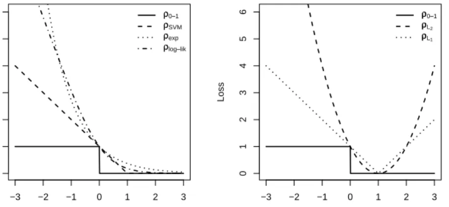
which then becomes an upper bound of the misclassification error, see Fig-ure1. Inmboost, the negative gradient of this loss function is implemented in a functionBinomial()returning an object of class boost family which con-tains the negative gradient function as a slot (assuming a binary response variabley∈ {−1,+1}).
The population minimizer can be shown to be [33, cf.] flog-lik∗ (x) = 1 2log p(x) 1−p(x) , p(x) =P[Y = 1|X =x].
The loss function in (3.1) is a function of ˜yf, the so-called margin value, where the functionf induces the following classifier forY:
C(x) = 1 iff(x)>0 0 iff(x)<0 undetermined iff(x) = 0.
Therefore, a misclassification (including the undetermined case) happens if and only if ˜Y f(X)≤0. Hence, the misclassification loss is
ρ0-1(y, f) =I{yf˜ ≤0},
(3.2)
whose population minimizer is equivalent to the Bayes classifier (for ˜Y ∈ {−1,+1})
f0-1∗ (x) =
(
+1 ifp(x)>1/2 −1 ifp(x)≤1/2,
where p(x) = P[Y = 1|X = x]. Note that the 0-1 loss in (3.2) cannot be used for boosting or FGD: it is non-differentiable and also non-convex as a function of the margin value ˜yf. The negative log-likelihood loss in (3.1) can be viewed as a convex upper approximation of the (computationally intractable) non-convex 0-1 loss, see Figure1. We will describe in Section3.3
the BinomialBoosting algorithm (similar to LogitBoost [33]) which uses the negative log-likelihood as loss function (i.e. the surrogate loss which is the implementing loss function for the algorithm).
Another upper convex approximation of the 0-1 loss function in (3.2) is the exponential loss
ρexp(y, f) = exp(−˜yf),
(3.3)
implemented (with notationy∈ {−1,+1}) in mboost asAdaExp()family. The population minimizer can be shown to be the same as for the log-likelihood loss [33, cf.]: fexp∗ (x) = 1 2log p(x) 1−p(x) , p(x) =P[Y = 1|X=x].
Using functional gradient descent with different (surrogate) loss functions yields different boosting algorithms. When using the log-likelihood loss in (3.1), we obtain LogitBoost [33] or BinomialBoosting from Section3.3; and with the exponential loss in (3.3), we essentially get AdaBoost [30] from Section1.2.
We interpret the boosting estimate ˆf[m](·) as an estimate of the
popula-tion minimizerf∗(·). Thus, the output from AdaBoost, Logit- or Binomial-Boosting are estimates of half of the log-odds ratio. In particular, we define probability estimates via
ˆ
p[m](x) = exp( ˆf
[m](x))
exp( ˆf[m](x)) + exp(−fˆ[m](x)).
The reason for constructing these probability estimates is based on the fact that boosting with a suitable stopping iteration is consistent [7, 51]. Some cautionary remarks about this line of argumentation are presented by Mease et al. [64].
Very popular in machine learning is the hinge function, the standard loss function for support vector machines:
ρSVM(y, f) = [1−yf˜ ]+,
where [x]+ =xI{x>0} denotes the positive part. It is also an upper convex
bound of the misclassification error, see Figure 1. Its population minimizer is
fSVM∗ (x) = sign(p(x)−1/2)
which is the Bayes classifier for ˜Y ∈ {−1,+1}. Since fSVM∗ (·) is a classi-fier and non-invertible function of p(x), there is no direct way to obtain conditional class probability estimates.
3.2. Regression. For regression with response Y ∈ R, we use most of-ten the squared error loss (scaled by the factor 1/2 such that the negative gradient vector equals the residuals, see Section3.3 below),
ρL2(y, f) =
1 2|y−f|
2
(3.4)
with population minimizer
−3 −2 −1 0 1 2 3 0 1 2 3 4 5 6 monotone ((2y−−1))f Loss ρρ0−−1 ρρSVM ρρexp ρρlog−−lik −3 −2 −1 0 1 2 3 0 1 2 3 4 5 6 non−monotone ((2y−−1))f Loss ρρ0−−1 ρρL2 ρρL1
Fig 1. Losses, as functions of the marginyf˜ = (2y−1)f, for binary classification.
Left panel with monotone loss functions: 0-1 loss, exponential loss, negative log-likelihood, hinge loss (SVM); right panel with non-monotone loss functions: squared
error (L2) and absolute error (L1) as in (3.5).
The corresponding boosting algorithm isL2Boosting, see Friedman [32] and
B¨uhlmann and Yu [22]. It is described in more detail in Section 3.3. This loss function is available inmboost as family GaussReg().
Alternative loss functions which have some robustness properties (with re-spect to the error distribution, i.e., in “Y-space”) include theL1- and
Huber-loss. The former is
ρL1(y, f) =|y−f|
with population minimizer
f∗(x) = median(Y|X=x) and is implemented inmboost asLaplace().
Although theL1-loss is not differentiable at the pointy=f, we can
com-pute partial derivatives since the single pointy =f (usually) has probability zero to be realized by the data. A compromise between the L1- andL2-loss
is the Huber-loss function from robust statistics:
ρHuber(y, f) =
(
|y−f|2/2, if|y−f| ≤δ
which is available inmboostasHuber(). A strategy for choosing (a changing)
δ adaptively has been proposed by Friedman [32]:
δm= median({|Yi−fˆ[m−1](Xi)|; i= 1, . . . , n}), where the previous fit ˆf[m−1](·) is used.
3.2.1. Connections to binary classification. Motivated from the popula-tion point of view, theL2- orL1-loss can also be used for binary classification.
ForY ∈ {0,1}, the population minimizers are
fL∗2(x) =E[Y|X =x] =p(x) =P[Y = 1|X =x],
fL∗1(x) = median(Y|X =x) =
(
1 ifp(x)>1/2 0 ifp(x)≤1/2.
Thus, the population minimizer of theL1-loss is the Bayes classifier.
Moreover, both the L1- and L2-loss functions can be parametrized as
functions of the margin value ˜yf (˜y∈ {−1,+1}): |˜y−f| = |1−yf˜ |,
|˜y−f|2 = |1−yf˜ |2= (1−2˜yf+ (˜yf)2.
(3.5)
The L1- and L2-loss functions are non-monotone functions of the margin
value ˜yf, see Figure 1. A negative aspect is that they penalize margin val-ues which are greater than 1: penalizing large margin valval-ues can be seen as a way to encourage solutions ˆf ∈ [−1,1] which is the range of the popula-tion minimizersfL∗1 and fL∗2 (for ˜Y ∈ {−1,+1}) , respectively. However, as discussed below, we prefer to use monotone loss functions.
The L2-loss for classification (with response variable y ∈ {−1,+1}) is
implemented inGaussClass().
All loss functions mentioned for binary classification (displayed in Fig-ure1) can be viewed and interpreted from the perspective of proper scoring rules, cf. Buja et al. [24]. We usually prefer the negative log-likelihood loss in (3.1) because: (i) it yields probability estimates; (ii) it is a monotone loss function of the margin value ˜yf; (iii) it grows linearly as the margin value ˜yf
tends to−∞, unlike the exponential loss in (3.3). The third point reflects a robustness aspect: it is similar to Huber’s loss function which also penalizes large values linearly (instead of quadratically as with theL2-loss).
3.3. Two important boosting algorithms. Table 1 summarizes the most popular loss functions and their corresponding boosting algorithms. We now describe the two algorithms appearing in the last two rows of Table1in more detail.
range spaces ρ(y, f) f∗(x) algorithm y∈ {0,1}, f∈R exp(−(2y−1)f) 12log
p(x) 1−p(x) AdaBoost y∈ {0,1}, f∈R log2(1 +e −2(2y−1)f) 1 2log p(x) 1−p(x) LogitBoost / BinomialBoosting y∈R, f∈R 12|y−f| 2 E[Y|X =x] L2Boosting Table 1
Various loss functionsρ(y, f), population minimizersf∗(x)and names of corresponding boosting algorithms;p(x) =P[Y = 1|X=x].
3.3.1. L2Boosting. L2Boosting is the simplest and perhaps most
instruc-tive boosting algorithm. It is very useful for regression, in particular in presence of very many predictor variables. Applying the general description of the FGD-algorithm from Section 2.1 to the squared error loss function
ρL2(y, f) =|y−f|
2/2, we obtain the following algorithm.
L2Boosting algorithm
1. Initialize ˆf[0](·) with an offset value. The default value is ˆf[0](·)≡Y. Setm= 0.
2. Increase m by 1. Compute the residuals Ui = Yi −fˆ[m−1](Xi) for
i= 1, . . . , n.
3. Fit the residual vector U1, . . . , Un to X1, . . . , Xn by the real-valued base procedure (e.g., regression)
(Xi, Ui)ni=1
base procedure
−→ gˆ[m](·).
4. Up-date ˆf[m](·) = ˆf[m−1](·)+ν·ˆg[m](·), where 0< ν ≤1 is a step-length factor (as in the general FGD-algorithm).
5. Iterate steps 2 to 4 untilm=mstop for some stopping iterationmstop.
The stopping iteration mstop is the main tuning parameter which can be
selected using cross-validation or some information criterion as described in Section5.4.
The derivation from the generic FGD algorithm in Section2.1is straight-forward. Note that the negative gradient vector becomes the residual vector. Thus,L2Boosting amounts to refitting residuals multiple times. Tukey [83]
recognized this to be useful and proposed “twicing” which is nothing else thanL2Boosting usingmstop= 2 (andν = 1).
3.3.2. BinomialBoosting: the FGD version of LogitBoost. We already gave some reasons at the end of Section3.2.1why the negative log-likelihood loss function in (3.1) is very useful for binary classification problems. Fried-man et al. [33] were first in advocating this, and they proposed LogitBoost
which is very similar to the generic FGD algorithm when using the loss from (3.1): the deviation from FGD is the use of Newton’s method involving the Hessian matrix (instead of a step-length for the gradient).
For the sake of coherence with the generic functional gradient descent algorithm in Section2.1, we describe here a version of LogitBoost: to avoid conflicting terminology, we coin it BinomialBoosting.
BinomialBoosting algorithm
Apply the generic FGD algorithm from Section2.1using the loss func-tion ρlog-lik from (3.1). The default offset value is ˆf[0](·) ≡log(ˆp/(1−
ˆ
p))/2, where ˆp is the relative frequency ofY = 1.
With BinomialBoosting, there is no need that the base procedure is able to do weighted fitting: this constitutes a slight difference to the requirement for LogitBoost [33].
3.4. Other data structures and models. Due to the generic nature of boosting or functional gradient descent, we can use the technique in very many other settings. For data with univariate responses and loss functions which are differentiable with respect to the second argument, the boosting algorithm is described in Section2.1. Survival analysis is an important area of application with censored observations: we describe in Section 8 how to deal with it.
4. Choosing the base procedure. Every boosting algorithm requires the specification of a base procedure. This choice can be driven by the aim of optimizing the predictive capacity only or by considering some structural properties of the boosting estimate in addition. We find the latter usually more interesting as it allows for better interpretation of the resulting model. We recall that the generic boosting estimator is a sum of base procedure estimates ˆ f[m](·) =ν m X k=1 ˆ g[k](·).
Therefore, structural properties of the boosting function estimator are in-duced by a linear combination of structural characteristics of the base pro-cedure.
The following important examples of base procedures yield useful struc-tures for the boosting estimator ˆf[m](·). The notation is as follows: ˆg(·) is an estimate from a base procedure which is based on data (X1, U1), . . . ,(Xn, Un) where (U1, . . . , Un) denotes the current negative gradient. In the sequel, the
4.1. Componentwise linear least squares for linear models. Boosting can be very useful for fitting potentially high-dimensional generalized linear mod-els. Consider the base procedure
ˆ g(x) = ˆβ( ˆS)x( ˆS), ˆ β(j)= n X i=1 Xi(j)Ui/ n X i=1 Xi(j)2, Sˆ= argmin 1≤j≤p n X i=1 Ui−βˆ(j)Xi(j) 2 . (4.1)
It selects the best variable in a simple linear model in the sense of ordinary least squares fitting.
When usingL2Boosting with this base procedure, we select in every
itera-tion one predictor variable, not necessarily a different one for each iteraitera-tion, and we up-date the function linearly:
ˆ
f[m](x) = ˆf[m−1](x) +νβˆ( ˆSm)x( ˆSm),
where ˆSm denotes the index of the selected predictor variable in iteration
m. Alternatively, the up-date of the coefficient estimates is ˆ
β[m]= ˆβ[m−1]+ν·βˆ( ˆSm).
The notation should be read that only the ˆSmth component of the coefficient estimate ˆβ[m] (in iteration m) has been up-dated. For every iteration m,
we obtain a linear model fit. As m tends to infinity, ˆf[m](·) converges to a least squares solution which is unique if the design matrix has full rank
p≤n. The method is also known as matching pursuit in signal processing [60], weak greedy algorithm in computational mathematics [81], and it is a Gauss-Southwell algorithm [79] for solving a linear system of equations. We will discuss more properties ofL2Boosting with componentwise linear least
squares in Section5.2.
When using BinomialBoosting with componentwise linear least squares from (4.1), we obtain a fit, including variable selection, of a linear logistic regression model.
As will be discussed in more detail in Section 5.2, boosting typically shrinks the (logistic) regression coefficients towards zero. Usually, we do not want to shrink the intercept term. In addition, we advocate to use boosting on mean centered predictor variables ˜Xi(j)=Xi(j)−X(j). In case of a linear model, when centering also the response ˜Yi =Yi−Y, this becomes
˜ Yi= p X j=1 β(j)X˜i(j)+ noisei
which forces the regression surface through the center (˜x(1), . . . ,x˜(p),y˜) = (0,0, . . . ,0) as with ordinary least squares. Note that it is not necessary to center the response variables when using the default offset value ˆf[0] =Y in
L2Boosting (for BinomialBoosting, we would center the predictor variables
only but never the response, and we would use ˆf[0] ≡argmincn−1
n
P
i=1
ρ(Yi, c)).
Illustration: Prediction of total body fat. Garcia et al. [34] report on the de-velopment of predictive regression equations for body fat content by means of p = 9 common anthropometric measurements which were obtained for
n = 71 healthy German women. In addition, the women’s body compo-sition was measured by Dual Energy X-Ray Absorptiometry (DXA). This reference method is very accurate in measuring body fat but finds little applicability in practical environments, mainly because of high costs and the methodological efforts needed. Therefore, a simple regression equation for predicting DXA measurements of body fat is of special interest for the practitioner. Backward-elimination was applied to select important variables from the available anthropometrical measurements and Garcia et al. [34] re-port a final linear model utilizing hip circumference, knee breadth and a compound covariate which is defined as the sum of log chin skinfold, log triceps skinfold and log subscapular skinfold:
R> bf_lm <- lm(DEXfat ~ hipcirc + kneebreadth + anthro3a, data = bodyfat)
R> coef(bf_lm)
(Intercept) hipcirc kneebreadth anthro3a
-75.23478 0.51153 1.90199 8.90964
A simple regression formula which is easy to communicate, such as a linear combination of only a few covariates, is of special interest in this applica-tion: we employ theglmboostfunction from package mboost to fit a linear regression model by means of L2Boosting with componentwise linear least
squares. By default, the functionglmboost fits a linear model (with initial
mstop = 100 and shrinkage parameterν = 0.1) by minimizing squared error
(argumentfamily = GaussReg() is the default):
R> bf_glm <- glmboost(DEXfat ~ ., data = bodyfat, control = boost_control(center = TRUE))
Note that, by default, the mean of the response variable is used as an offset in the first step of the boosting algorithm. We center the covariates prior to model fitting in addition. As mentioned above, the special form of the base learner, i.e., componentwise linear least squares, allows for a reformulation
of the boosting fit in terms of a linear combination of the covariates which can be assessed via
R> coef(bf_glm)
(Intercept) age waistcirc hipcirc
0.000000 0.013602 0.189716 0.351626
elbowbreadth kneebreadth anthro3a anthro3b
-0.384140 1.736589 3.326860 3.656524
anthro3c anthro4
0.595363 0.000000
attr(,"offset") [1] 30.783
We notice that most covariates have been used for fitting and thus no ex-tensive variable selection was performed in the above model. Thus, we need to investigate how many boosting iterations are appropriate. Resampling methods such as cross-validation or the bootstrap can be used to estimate the out-of-sample error for a varying number of boosting iterations. The out-of-bootstrap mean squared error for 100 bootstrap samples is depicted in the upper part of Figure2. The plot leads to the impression that approx-imately mstop = 44 would be a sufficient number of boosting iterations. In
Section5.4, a corrected version of the Akaike information criterion (AIC) is proposed for determining the optimal number of boosting iterations. This criterion attains its minimum for
R> mstop(aic <- AIC(bf_glm))
[1] 45
boosting iterations, see the bottom part of Figure 2 in addition. The coef-ficients of the linear model withmstop = 45 boosting iterations are
R> coef(bf_glm[mstop(aic)])
(Intercept) age waistcirc hipcirc
0.0000000 0.0023271 0.1893046 0.3488781
elbowbreadth kneebreadth anthro3a anthro3b
0.0000000 1.5217686 3.3268603 3.6051548
anthro3c anthro4
0.5043133 0.0000000
attr(,"offset") [1] 30.783
and thus 7 covariates have been selected for the final model (intercept equal to zero occurs here for mean centered response and predictors and hence,
n−1Pn
i=1Yi = 30.783 is the intercept in the uncentered model). Note that the variableshipcirc,kneebreadthandanthro3a, which we have used for
Number of boosting iterations
Out−of−bootstrap squared error
2 8 16 24 32 40 48 56 64 72 80 88 96 0 20 40 60 80 100 120 140 ● 0 20 40 60 80 100 3.0 3.5 4.0 4.5 5.0 5.5
Number of boosting iterations
Corrected AIC
●
Fig 2.bodyfatdata: Out-of-bootstrap squared error for varying number of boosting
itera-tionsmstop (top). The dashed horizontal line depicts the average out-of-bootstrap error of the linear model for the pre-selected variableshipcirc, kneebreadthand anthro3afitted via ordinary least squares. The lower part shows the corrected AIC criterion.
fitting a linear model at the beginning of this paragraph, have been selected by the boosting algorithm as well.
4.2. Componentwise smoothing spline for additive models. Additive and generalized additive models, introduced by Hastie and Tibshirani [40] (see also [41]), have become very popular for adding more flexibility to the linear structure in generalized linear models. Such flexibility can also be added in boosting (whose framework is especially useful for high-dimensional prob-lems).
We can choose use a nonparametric base procedure for function estima-tion. Suppose that
ˆ
f(j)(·) is a least squares cubic smoothing spline estimate based on
U1, . . . , Un against X1(j), . . . , X (j)
n with fixed degrees of freedom df. (4.2) That is, ˆ f(j)(·) = argmin f(·) n X i=1 Ui−f Xi(j)2+λ Z (f00(x))2dx, (4.3)
whereλ >0 is a tuning parameter such that the trace of the corresponding hat matrix equals df. For further details, we refer to Green and Silverman [36]. As a note of caution, we use in the sequel the terminology of “hat matrix” in a broad sense: it is a linear operator but not a projection in general.
The base procedure is then ˆ
g(x) = ˆf( ˆS)(x( ˆS)),
ˆ
f(j)(·) as above and ˆS = argmin
1≤j≤p n X i=1 Ui−fˆ(j)(Xi(j)) 2 ,
where the degrees of freedom df are the same for all ˆf(j)(·).
L2Boosting with componentwise smoothing splines yields an additive model,
including variable selection, i.e., a fit which is additive in the predictor vari-ables. This can be seen immediately sinceL2Boosting proceeds additively for
up-dating the function ˆf[m](·), see Section 3.3. We can normalize to obtain the following additive model estimator:
ˆ f[m](x) = ˆµ+ p X j=1 ˆ f[m],(j)x(j), n−1 n X i=1 ˆ f[m],(j)Xi(j)= 0 for all j= 1, . . . , p.
As with the componentwise linear least squares base procedure, we can use componentwise smoothing splines also in BinomialBoosting, yielding an ad-ditive logistic regression fit.
The degrees of freedom in the smoothing spline base procedure should be chosen “small” such as df = 4. This yields low variance but typically large bias of the base procedure. The bias can then be reduced by additional boosting iterations. This choice of low variance but high bias has been analyzed in B¨uhlmann and Yu [22], see also Section4.4.
Componentwise smoothing splines can be generalized to pairwise smooth-ing splines which searches for and fits the best pairs of predictor variables such that a smooth ofU1, . . . , Un against this pair of predictors reduces the residual sum of squares most. WithL2Boosting, this yields a nonparametric
model fit with first order interaction terms. The procedure has been empir-ically demonstrated to be often much better than fitting with MARS [23].
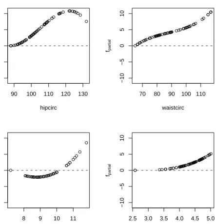
Illustration: Prediction of total body fat (cont.). Being more flexible than the linear model which we fitted to the bodyfat data in Section 4.1, we estimate an additive model using thegamboostfunction frommboost (first with pre-specified mstop = 100 boosting iterations, ν = 0.1 and squared
error loss):
R> bf_gam <- gamboost(DEXfat ~ ., data = bodyfat)
The degrees of freedom in the componentwise smoothing spline base proce-dure can be defined by thedfbase argument, defaulting to 4.
We can estimate the number of boosting iterations mstop using the
cor-rected AIC criterion described in Section5.4 via
R> mstop(aic <- AIC(bf_gam))
[1] 46
Similar to the linear regression model, the partial contributions of the co-variates can be extracted from the boosting fit. For the most important vari-ables, the partial fits are given in Figure3showing some slight non-linearity, mainly forkneebreadth.
4.3. Trees. In the machine learning community, regression trees are the most popular base procedures. They have the advantage to be invariant un-der monotone transformations of predictor variables, i.e., we do not need to search for good data transformations. Moreover, regression trees handle covariates measured at different scales (continuous, ordinal or nominal vari-ables) in a unified way; unbiased split or variable selection in the context of different scales is proposed in [47].
● ● ● ● ● ● ●● ● ● ● ●● ● ●● ● ● ● ● ● ● ● ● ● ● ● ● ● ● ●● ● ● ● ●● ● ● ● ● ● ● ● ● ●● ● ● ● ● ● ● ● ● ● ● ● ● ● ●● ● ●● ● ●● ● ● ● 90 100 110 120 130 −5 0 5 hipcirc fpa rt ia l ●●● ● ● ● ● ● ● ● ● ● ● ● ● ● ● ● ● ● ● ● ●● ● ●● ● ● ● ●● ● ● ● ● ● ● ● ● ● ● ● ● ● ● ●● ● ● ● ● ● ● ● ●● ● ● ● ● ● ●● ● ● ●● ● ● ● 70 80 90 100 110 −5 0 5 waistcirc fpa rt ia l ● ● ●● ● ●● ● ●●●● ● ● ● ● ● ● ● ● ● ● ● ● ● ● ● ● ● ● ● ● ● ● ● ● ● ● ● ● ● ● ● ● ● ● ● ● ● ● ● ● ● ● ● ● ● ● ● ● ● ● ●●●●●●●●● 8 9 10 11 −5 0 5 kneebreadth fpa rt ia l ●● ● ● ● ● ● ● ● ●● ●● ● ● ● ● ● ● ● ● ● ● ● ● ● ● ● ● ● ● ● ●● ● ● ● ● ● ● ● ● ● ● ● ●● ● ● ● ● ● ● ● ● ● ● ● ● ● ● ● ● ● ● ● ● ● ● ● ● 2.5 3.0 3.5 4.0 4.5 5.0 −5 0 5 anthro3b fpa rt ia l
Fig 3.bodyfatdata: Partial contributions of four covariates in an additive model (without
centering of estimated functions to mean zero).
When using stumps, i.e., a tree with two terminal nodes only, the boost-ing estimate will be an additive model in the original predictor variables, because every stump-estimate is a function of a single predictor variable only. Similarly, boosting trees with (at most) dterminal nodes results in a nonparametric model having at most interactions of orderd−2. Therefore, if we want to constrain the degree of interactions, we can easily do this by constraining the (maximal) number of nodes in the base procedure.
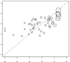
Illustration: Prediction of total body fat (cont.). Both thegbmpackage [74] and the mboost package are helpful when decision trees are to be used as base procedures. Inmboost, the function blackboostimplements boosting
●● ● ● ● ● ● ● ● ● ● ● ● ● ● ● ● ● ● ● ● ● ● ● ● ● ● ● ● ● ●● ● ● ● ● ● ● ● ● ● ● ● ● ● ● ● ● ● ● ● ● ● ● ● ● ● ● ● ● ●● ●● ● ● ● ● ● ● ● 10 20 30 40 50 60 10 20 30 40 50 60 Prediction gbm Prediction blackboost
Fig 4. bodyfat data: Fitted values of both the gbm and mboost implementations of
L2Boosting with different regression trees as base learners.
for fitting such classicalblack-box models:
R> bf_black <- blackboost(DEXfat ~ ., data = bodyfat, control = boost_control(mstop = 500))
Conditional inference trees [47] as available from thepartypackage [46] are utilized as base procedures. Here, the function boost_control defines the number of boosting iterationsmstop.
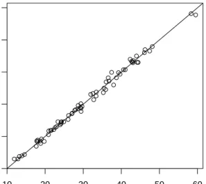
Alternatively, we can use the function gbm from the gbm package which yields roughly the same fit as can be seen from Figure4.
4.4. The low-variance principle. We have seen above that the structural properties of a boosting estimate are determined by the choice of a base pro-cedure. In our opinion, the structure specification should come first. After having made a choice, the question becomes how “complex” the base proce-dure should be. For example, how should we choose the degrees of freedom for the componentwise smoothing spline in (4.2)? A general answer is: choose the base procedure (having the desired structure) with low variance at the price of larger estimation bias. For the componentwise smoothing splines,
this would imply a low number of degrees of freedom, e.g., df = 4.
We give some reasons for the low-variance principle in Section5.1(Replica1). Moreover, it has been demonstrated in Friedman [32] that a small step-size factor ν can be often beneficial and almost never yields substantially worse predictive performance of boosting estimates. Note that a small step-size factor can be seen as a shrinkage of the base procedure by the factor ν, implying low variance but potentially large estimation bias.
5. L2Boosting. L2Boosting is functional gradient descent using the
squared error loss which amounts to repeated fitting of ordinary residuals, as described already in Section 3.3.1. Here, we aim at increasing the un-derstanding of the simple L2Boosting algorithm. We first start with a toy
problem of curve estimation, and we will then illustrate concepts and re-sults which are especially useful for high-dimensional data. These can serve as heuristics for boosting algorithms with other convex loss functions for problems in e.g., classification or survival analysis.
5.1. Nonparametric curve estimation: from basics to asymptotic optimal-ity. Consider the toy problem of estimating a regression functionE[Y|X=
x] with one-dimensional predictorX∈Rand a continuous responseY ∈R. Consider the case with a linear base procedure having a hat matrix H :Rn → Rn, mapping the response variables Y = (Y1, . . . , Yn)> to their
fitted values ( ˆf(X1), . . . ,fˆ(Xn))>. Examples include nonparametric kernel smoothers or smoothing splines. It is easy to show that the hat matrix of the L2Boosting fit (for simplicity, with ˆf[0] ≡ 0 and ν = 1) in iteration m
equals:
Bm=Bm−1+H(I− Bm−1) =I −(I− H)m.
(5.1)
Formula (5.1) allows for several insights. First, if the base procedure satisfies kI − Hk < 1 for a suitable norm, i.e., has a “learning capacity” such that the residual vector is shorter than the input-response vector, we see that Bm converges to the identity I asm→ ∞, and BmY converges to the fully saturated model Y, interpolating the response variables exactly. Thus, we see here explicitly that we have to stop early with the boosting iterations in order to prevent over-fitting.
When specializing to the case of a cubic smoothing spline base procedure (cf. Formula (4.3)), it is useful to invoke some eigen-analysis. The spectral representation is
where λ1 ≥ λ2 ≥ . . . ≥ λn denote the (ordered) eigenvalues of H. It then follows with (5.1) that
Bm=U DmU>,
Dm= diag(d1,m, . . . , dn,m), di,m = 1−(1−λi)m. It is well known that a smoothing spline satisfies:
λ1 =λ2= 1, 0< λi <1 (i= 3, . . . , n).
Therefore, the eigenvalues of the boosting hat operator (matrix) in iteration
m satisfy:
d1,m≡d2,m≡1 for all m, (5.2)
0< di,m = 1−(1−λi)m<1 (i= 3, . . . , n), di,m→1 (m→ ∞). (5.3)
When comparing the spectrum, i.e., the set of eigenvalues, of a smoothing spline with its boosted version, we have the following. For both cases, the largest two eigenvalues are equal to 1. Moreover, all other eigenvalues can be changed by either varying the degrees of freedom df =Pn
i=1λi in a single smoothing spline, or by varying the boosting iteration m with some fixed (low-variance) smoothing spline base procedure having fixed (low) values
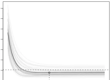
λi. In Figure 5 we demonstrate the difference between the two approaches for changing “complexity” of the estimated curve fit by means of a toy ex-ample first shown in [22]. Both methods have about the same minimum mean squared error butL2Boosting overfits much more slowly than a single
smoothing spline.
By careful inspection of the eigen-analysis for this simple case of boosting a smoothing spline, B¨uhlmann and Yu [22] proved an asymptotic minimax rate result:
Replica 1. [22] When stopping the boosting iterations appropriately, i.e., mstop = mn = O(n4/(2ξ+1)), mn → ∞ (n → ∞) with ξ ≥ 2 as
be-low, L2Boosting with cubic smoothing splines having fixed degrees of
free-dom achieves the minimax convergence rate over Sobolev function classes of smoothness degree ξ≥2, as n→ ∞.
Two items are interesting. First, minimax rates are achieved by using a base procedure with fixed degrees of freedom which means low variance from an asymptotic perspective. Secondly, L2Boosting with cubic
smooth-ing splines has the capability to adapt to higher order smoothness of the true underlying function: thus, with the stopping iteration as the one and
● ● ● ● ●●● ●●●●●●●●●●●●●●●●●● 0 200 400 600 800 1000 0.0 0.2 0.4 0.6 0.8 Boosting
Number of boosting iterations
Mean squared error
● ●●● ● ● ● ● ● ● ● ● ● ● ● ● ● ● ● ● 10 20 30 40 0.0 0.2 0.4 0.6 0.8 Smoothing Splines Degrees of freedom
Fig 5. Mean squared prediction error E[(f(X)−f(Xˆ ))2]for the regression model Yi =
0.8Xi+ sin(6Xi) +εi (i= 1, . . . , n = 100), with ε ∼ N(0,2), Xi ∼ U(−1/2,1/2), av-eraged over 100simulation runs. Left: L2Boosting with smoothing spline base procedure (having fixed degrees of freedom df = 4) and usingν= 0.1, for varying number of boosting iterations. Right: single smoothing spline with varying degrees of freedom.
only tuning parameter, we can nevertheless adapt to any higher-order de-gree of smoothness (without the need of choosing a higher order spline base procedure).
Recently, asymptotic convergence and minimax rate results have been established for early-stopped boosting in more general settings [10,91].
5.1.1. L2Boosting using kernel estimators. As we have pointed out in
Replica1,L2Boosting of smoothing splines can achieve faster mean squared
error convergence rates than the classicalO(n−4/5), assuming that the true underlying function is sufficiently smooth. We illustrate here a related phe-nomenon with kernel estimators.
We consider fixed, univariate design pointsxi =i/n(i= 1, . . . , n) and the Nadaraya-Watson kernel estimator for the nonparametric regression function E[Y|X=x]: ˆ g(x;h) = (nh)−1 n X i=1 K x−x i h Yi=n−1 n X i=1 Kh(x−xi)Yi,
where h > 0 is the bandwidth, K(·) a kernel in the form of a probability density which is symmetric around zero and Kh(x) = h−1K(x/h). It is straightforward to derive the form of L2Boosting using m = 2 iterations
(with ˆf[0] ≡ 0 and ν = 1), i.e., twicing [83], with the Nadaraya-Watson kernel estimator: ˆ f[2](x) = (nh)−1 n X i=1 Khtw(x−xi)Yi, Khtw(u) = 2Kh(u)−Kh∗Kh(u), whereKh∗Kh(u) =n−1 n X r=1 Kh(u−xr)Kh(xr).
For fixed design pointsxi=i/n, the kernel Khtw(·) is asymptotically equiv-alent to a higher-order kernel (which can take negative values) yielding a squared bias term of order O(h8), assuming that the true regression func-tion is four times continuously differentiable. Thus, twicing or L2Boosting
with m = 2 iterations amounts to be a Nadaraya-Watson kernel estimator with a higher-order kernel. This explains from another angle why boosting is able to improve the mean squared error rate of the base procedure. More de-tails including also non-equispaced designs are given in DiMarzio and Taylor [27].
5.2. L2Boosting for high-dimensional linear models. Consider a
poten-tially high-dimensional linear model
Yi=β0+ p X j=1 β(j)Xi(j)+εi, i= 1, . . . , n, (5.4)
whereε1, . . . , εn are i.i.d. withE[εi] = 0 and independent from allXi’s. We allow for the number of predictorspto be much larger than the sample sizen. The model encompasses the representation of a noisy signal by an expansion with an over-complete dictionary of functions {g(j)(·) : j = 1, . . . , p}; e.g., for surface modeling with design points inZi∈R2,
Yi=f(Zi) +εi, f(z) =
X
j
β(j)g(j)(z) (z∈R2).
Fitting the model (5.4) can be done usingL2Boosting with the
componen-twise linear least squares base procedure from Section4.1which fits in every iteration the best predictor variable reducing the residual sum of squares most. This method has the following basic properties:
1. As the number m of boosting iterations increases, theL2Boosting
es-timate ˆf[m](·) converges to a least squares solution. This solution is unique if the design matrix has full rank p≤n.
2. When stopping early which is usually needed to avoid over-fitting, the
3. The coefficient estimates ˆβ[m] are (typically) shrunken versions of a least squares estimate ˆβOLS, related to the Lasso as described in
Sec-tion5.2.1.
Illustration: Breast cancer subtypes. Variable selection is especially impor-tant in high-dimensional situations. As an example, we study a binary clas-sification problem involvingp= 7129 gene expression levels inn= 49 breast cancer tumor samples [data taken from 90]. For each sample, a binary re-sponse variable describes the lymph node status (25 negative and 24 posi-tive).
The data are stored in form of anexprSet objectwestbc [see35] and we first extract the matrix of expression levels and the response variable:
R> x <- t(exprs(westbc)) R> y <- pData(westbc)$nodal.y
We aim at using L2Boosting for classification, see Section 3.2.1, with
clas-sical AIC based on the binomial log-likelihood for stopping the boosting iterations. Thus, we first transform the factoryto a numeric variable with 0/1 coding:
R> yfit <- as.numeric(y) - 1
The general framework implemented inmboostallows us to specify the nega-tive gradient (thengradientargument) corresponding to the surrogate loss function, here the squared error loss implemented as a function rho, and a different evaluating loss function (the loss argument), here the negative binomial log-likelihood, with the Familyfunction as follows:
R> rho <- function(y, f, w = 1) {
p <- pmax(pmin(1 - 1e-05, f), 1e-05) -y * log(p) - (1 - y) * log(1 - p) }
R> ngradient <- function(y, f, w = 1) y - f R> offset <- function(y, w) weighted.mean(y, w) R> L2fm <- Family(ngradient = ngradient, loss = rho,
offset = offset)
The resulting object (calledL2fm), bundling the negative gradient, the loss function and a function for computing an offset term (offset), can now be passed to theglmboostfunction for boosting with componentwise linear least squares (here initialmstop = 200 iterations are used):
R> ctrl <- boost_control(mstop = 200, center = TRUE)
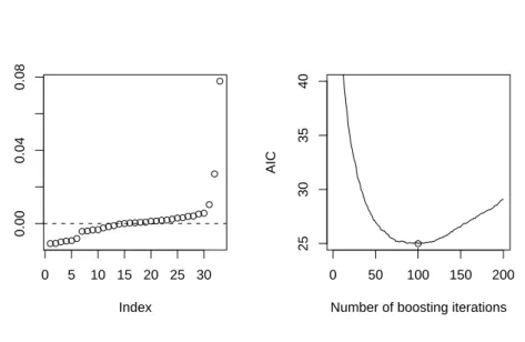
●●●●●● ●●●●●●●●●●● ●●●●●●●●●●●● ● ● ● ● 0 5 10 15 20 25 30 0.00 0.04 0.08 Index Standardized coefficients 0 50 100 150 200 25 30 35 40
Number of boosting iterations
AIC
●
Fig 6. westbc data: Standardized regression coefficientsβˆ(j)
q d
Var(X(j))(left panel) for
mstop= 100determined from the classical AIC criterion shown in the right panel.
Fitting such a linear model top = 7129 covariates for n= 49 observations takes about 3.6 seconds on a medium scale desktop computer (Intel Pentium 4, 2.8GHz). Thus, this form of estimation and variable selection is computa-tionally very efficient. As a comparison, computing all Lasso solutions, using package lars[28,39] inR(with use.Gram=FALSE), takes about 6.7 seconds. The question how to choose mstop can be addressed by the classical AIC
criterion as follows
R> aic <- AIC(west_glm, method = "classical") R> mstop(aic)
[1] 100
where the AIC is computed as -2(log-likelihood) + 2(degrees of freedom) = 2 (evaluating loss) + 2(degrees of freedom), see Formula (5.8). The notion of degrees of freedom is discussed in Section5.3.
Figure 6 shows the AIC curve depending on the number of boosting it-erations. When we stop after mstop = 100 boosting iterations, we obtain
33 genes with non-zero regression coefficients whose standardized values ˆ
β(j) q
d
Var(X(j)) are depicted in the left panel of Figure6.
Of course, we could also use BinomialBoosting for analyzing the data: the computational CPU time would be of the same order of magnitude, i.e., only a few seconds.
5.2.1. Connections to the Lasso. Hastie et al. [42] pointed out first an intriguing connection between L2Boosting with componentwise linear least
squares and the Lasso [82] which is the following `1-penalty method:
ˆ β(λ) = argmin β n−1 n X i=1 Yi−β0− p X j=1 β(j)Xi(j) 2 +λ p X j=1 |β(j)|. (5.5)
Efron et al. [28] made the connection rigorous and explicit: they consider a version of L2Boosting, called forward stagewise linear regression (FSLR),
and they show that FSLR with infinitesimally small step-sizes (i.e., the value
ν in step 4 of the L2Boosting algorithm in Section 3.3.1) produces a set of
solutions which is approximately equivalent to the set of Lasso solutions when varying the regularization parameterλin Lasso (see (5.5) above). The approximate equivalence is derived by representing FSLR and Lasso as two different modifications of the computationally efficient least angle regres-sion (LARS) algorithm from Efron et al. [28] (see also [68] for generalized linear models). The latter is very similar to the algorithm proposed earlier by Osborne et al. [67]. In special cases where the design matrix satisfies a “positive cone condition”, FSLR, Lasso and LARS all coincide [28, p.425]. For more general situations, when adding some backward steps to boosting, such modifiedL2Boosting coincides with the Lasso (Zhao and Yu [93]).
Despite the fact that L2Boosting and Lasso are not equivalent methods
in general, it may be useful to interpret boosting as being “related” to `1 -penalty based methods.
5.2.2. Asymptotic consistency in high dimensions. We review here a re-sult establishing asymptotic consistency for very high-dimensional but sparse linear models as in (5.4). To capture the notion of high-dimensionality, we equip the model with a dimensionality p = pn which is allowed to grow with sample sizen; moreover, the coefficientsβ(j)=β(nj)are now potentially depending onnand the regression function is denoted by fn(·).
Replica 2. [18] Consider the linear model in (5.4). Assume thatpn=
O(exp(n1−ξ)) for some0< ξ ≤1 (high-dimensionality) and sup n∈N
pn P
j=1
|β(nj)|< ∞(sparseness of the true regression function w.r.t. the `1-norm); moreover, the variablesXi(j) are bounded and E[|εi|4/ξ]<∞. Then: when stopping the
boosting iterations appropriately, i.e., m = mn → ∞ (n → ∞) sufficiently
slowly, L2Boosting with componentwise linear least squares satisfies
EXnew[( ˆf [mn]
where Xnew denotes new predictor variables, independent of and with the
same distribution as the X-component of the data (Xi, Yi) (i= 1, . . . , n). The result holds for almost arbitrary designs and no assumptions about collinearity or correlations are required. Replica 2 identifies boosting as a method which is able to consistently estimate a very high-dimensional but sparse linear model; for the Lasso in (5.5), a similar result holds as well [37]. In terms of empirical performance, there seems to be no overall superiority ofL2Boosting over Lasso or vice-versa.
5.2.3. Transforming predictor variables. In view of Replica 2, we may enrich the design matrix in model (5.4) with many transformed predictors: if the true regression function can be represented as a sparse linear combi-nation of original or transformed predictors, consistency is still guaranteed. It should be noted though that the inclusion of non-effective variables in the design matrix does degrade the finite-sample performance to a certain extent.
For example, higher order interactions can be specified in generalized AN(C)OVA models andL2Boosting with componentwise linear least squares
can be used to select a small number out of potentially many interaction terms.
As an option for continuously measured covariates, we may utilize a B-spline basis as illustrated in the next paragraph. We emphasize that during the process ofL2Boosting with componentwise linear least squares,
individ-ual spline basis functions from various predictor variables are selected and fitted one at a time; in contrast, L2Boosting with componentwise
smooth-ing splines fits a whole smoothsmooth-ing spline function (for a selected predictor variable) at a time.
Illustration: Prediction of total body fat (cont.). Such transformations and estimation of a corresponding linear model can be done with theglmboost
function, where the model formula performs the computations of all trans-formations by means of the bs (B-spline basis) function from the package splines. First, we set up a formula transforming each covariate
R> bsfm
DEXfat ~ bs(age) + bs(waistcirc) + bs(hipcirc) + bs(elbowbreadth) + bs(kneebreadth) + bs(anthro3a) + bs(anthro3b) + bs(anthro3c) + bs(anthro4)
and then fit the complex linear model by using theglmboostfunction with initialmstop = 5000 boosting iterations:
R> ctrl <- boost_control(mstop = 5000)
R> bf_bs <- glmboost(bsfm, data = bodyfat, control = ctrl) R> mstop(aic <- AIC(bf_bs))
[1] 2891
The corrected AIC criterion (see Section5.4) suggests to stop aftermstop =
2891 boosting iterations and the final model selects 21 (transformed) pre-dictor variables. Again, the partial contributions of each of the 9 original covariates can be computed easily and are shown in Figure 7(for the same variables as in Figure3). Note that the depicted functional relationship de-rived from the model fitted above (Figure7) is qualitatively the same as the one derived from the additive model (Figure3).
5.3. Degrees of freedom for L2Boosting. A notion of degrees of freedom
will be useful for estimating the stopping iteration of boosting (Section5.4). 5.3.1. Componentwise linear least squares. We considerL2Boosting with
componentwise linear least squares. Denote by
H(j)=X(j)(X(j))>/kX(j)k2, j = 1, . . . , p,
then×nhat matrix for the linear least squares fitting operator using thejth predictor variable X(j) = (X1(j), . . . , Xn(j))> only; kxk2 = x>x denotes the Euclidean norm for a vectorx ∈Rn. The hat matrix of the componentwise linear least squares base procedure (see (4.1)) is then
H( ˆS) : (U1, . . . , Un)7→Uˆ1, . . . ,Uˆn,
where ˆS is as in (4.1). Similarly to (5.1), we then obtain the hat matrix of
L2Boosting in iteration m:
Bm = Bm−1+ν· H( ˆSm)(I− Bm−1)
= I−(I−νH( ˆSm))(I−νH( ˆSm−1))· · ·(I−νH( ˆS1)),
(5.6)
where ˆSr ∈ {1, . . . , p}denotes the component which is selected in the com-ponentwise least squares base procedure in the rth boosting iteration. We emphasize thatBm is depending on the response variableY via the selected components ˆSr, r = 1, . . . m. Due to this dependence onY,Bm should be viewed as an approximate hat matrix only. Neglecting the selection effect of ˆSr (r = 1, . . . m), we define the degrees of freedom of the boosting fit in iterationm as
● ● ● ● ● ● ●● ● ● ● ●● ● ●● ● ● ● ● ● ● ● ● ● ● ● ● ● ● ● ● ● ● ● ●● ● ● ● ● ● ● ● ● ●● ● ● ● ● ● ● ● ● ● ● ● ● ● ●● ● ● ● ● ●● ● ● ● 90 100 110 120 130 −10 −5 0 5 10 hipcirc fpa rt ia l ● ● ● ● ● ● ● ● ● ● ● ● ● ● ● ● ● ● ● ● ● ● ●● ● ● ● ● ● ● ●● ● ● ● ● ● ● ● ● ● ● ● ● ● ●●● ● ● ● ● ● ● ● ●● ● ● ● ● ● ●● ● ● ●● ● ● ● 70 80 90 100 110 −10 −5 0 5 10 waistcirc fpa rt ia l ● ● ● ● ● ●● ● ●●●● ● ● ● ●● ● ● ● ● ● ● ● ● ● ● ● ● ● ● ● ● ● ● ● ● ● ● ● ● ● ● ● ● ● ● ● ● ● ● ● ● ● ● ● ● ● ● ● ● ● ●●●● ● ● ●● ● 8 9 10 11 −10 −5 0 5 10 kneebreadth fpa rt ia l ●● ● ● ● ● ● ● ● ●● ●● ● ● ● ● ● ● ● ● ● ● ● ● ● ● ● ● ● ● ● ●● ● ● ● ● ● ● ● ● ● ●●●● ● ● ● ● ● ● ● ● ● ● ● ● ● ● ● ● ● ● ● ● ● ● ● ● 2.5 3.0 3.5 4.0 4.5 5.0 −10 −5 0 5 10 anthro3b fpa rt ia l
Fig 7. bodyfatdata: Partial fits for a linear model fitted to transformed covariates using
B-splines (without centering of estimated functions to mean zero).
Even withν = 1, df(m) is very different from counting the number of vari-ables which have been selected until iteration m.
Having some notion of degrees of freedom at hand, we can estimate the error varianceσε2=E[ε2i] in the linear model (5.4) by
ˆ σ2ε = 1 n−df(mstop) n X i=1 Yi−fˆ[mstop](Xi) 2 .
Moreover, we can represent Bm= p X j=1 Bm(j), (5.7)
whereB(mj) is the (approximate) hat matrix which yields the fitted values for thejth predictor, i.e., Bm(j)Y =X(j)βˆj[m]. Note that the B(mj)’s can be easily computed in an iterative way by up-dating as follows:
B( ˆmSm) =B( ˆSm)
m−1 +ν· H( ˆ
Sm)(I− B
m−1),
Bm(j)=Bm(j−)1 for all j6= ˆSm.
Thus, we have a decomposition of the total degrees of freedom intopterms: df(m) = p X j=1 df(j)(m), df(j)(m) = trace(B(mj)).
The individual degrees of freedom df(j)(m) are a useful measure to quantify the “complexity” of the individual coefficient estimate ˆβj[m].
5.4. Internal stopping criteria for L2Boosting. Having some degrees of
freedom at hand, we can now use information criteria for estimating a good stopping iteration, without pursuing some sort of cross-validation.
We can use the corrected AIC [49]:
AICc(m) = log(ˆσ2) + 1 + df(m)/n (1−df(m) + 2)/n, ˆ σ2 =n−1 n X i=1 (Yi−(BmY)i)2.
Inmboost, the corrected AIC criterion can be computed viaAIC(x, method = "corrected") (with x being an object returned by glmboost or gam-boost called with family = GaussReg()). Alternatively, we may employ the gMDL criterion (Hansen and Yu [38]):
gMDL(m) = log(S) +df(m) n log(F), S= nσˆ 2 n−df(m), F = Pn i=1Yi2−nσˆ2 df(m)S .
The gMDL criterion bridges the AIC and BIC in a data-driven way: it is an attempt to adaptively select the better among the two.
When usingL2Boosting for binary classification (see also the end of
binomial log-likelihood in AIC, AIC(m) = −2 n X i=1 Yilog ((BmY)i) (5.8) + (1−Yi) log (1−(BmY)i) + 2df(m),
or for BIC(m) with the penalty term log(n)df(m). (If (BmY)i ∈/ [0,1], we truncate by max(min((BmY)i,1−δ), δ) for some smallδ >0. e.g.,δ= 10−5).
6. Boosting for variable selection. We address here the question whether boosting is a good variable selection scheme. For problems with many predictor variables, boosting is computationally much more efficient than classical all subset selection schemes. The mathematical properties of boosting for variable selection are still open questions, e.g., whether it leads to a consistent model selection method.
6.1. L2Boosting. When borrowing from the analogy ofL2Boosting with
the Lasso (see Section 5.2.1), the following is relevant. Consider a linear model as in (5.4), allowing for p n but being sparse. Then, there is a sufficient and “almost” necessary neighborhood stability condition (the word “almost” refers to a strict inequality “<” whereas “≤” suffices for sufficiency) such that for some suitable penalty parameter λ in (5.5), the Lasso finds the true underlying sub-model (the predictor variables with corresponding regression coefficients6= 0) with probability tending quickly to 1 as n→ ∞ [65]. It is important to note the role of the sufficient and “almost” necessary condition of the Lasso for model selection: Zhao and Yu [94] call it the “irrepresentable condition” which has (mainly) implications on the “degree of collinearity” of the design (predictor variables), and they give examples where it holds and where it fails to be true. A further complication is the fact that when tuning the Lasso for prediction optimality, i.e., choosing the penalty parameterλ in (5.5) such that the mean squared error is minimal, the probability for estimating the true sub-model converges to a number which is less than one or even zero if the problem is high-dimensional [65]. In fact, the prediction optimal tuned Lasso selects asymptotically too large models.
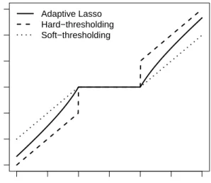
The bias of the Lasso mainly causes the difficulties mentioned above. We often would like to construct estimators which are less biased. It is instructive to look at regression with orthonormal design, i.e., the model (5.4) withPn
i=1X (j)
i X
(k)
i =δjk. Then, the Lasso and also L2Boosting with
componentwise linear least squares and using very small ν (in step 4 of
see Figure 8. It exhibits the same amount of bias regardless by how much the observation (the variable z in Figure 8) exceeds the threshold. This is in contrast to the hard-threshold estimator and the adaptive Lasso in (6.1) which are much better in terms of bias.
−3 −2 −1 0 1 2 3 −3 −2 −1 0 1 2 3 z 0 Adaptive Lasso Hard−thresholding Soft−thresholding
Fig 8. Hard-threshold (dotted-dashed), soft-threshold (dotted) and adaptive Lasso
(solid) estimator in a linear model with orthonormal design. For this design, the
adaptive Lasso coincides with the non-negative garrote [13]. The value on the
x-abscissa, denoted by z, is a single component ofX>Y.
Nevertheless, the (computationally efficient) Lasso seems to be a very useful method for variable filtering: for many cases, the prediction optimal tuned Lasso selects a sub-model which contains the true model with high probability. A nice proposal to correct Lasso’s over-estimation behavior is the adaptive Lasso, given by Zou [96]. It is based on re-weighting the penalty function. Instead of (5.5), the adaptive Lasso estimator is
ˆ β(λ) = argmin β n−1 n X i=1 Yi−β0− p X j=1 β(j)Xi(j) 2 (6.1) +λ p X j=1 |β(j)| |βˆinit(j)|,

![Fig 5. Mean squared prediction error E[(f (X) − ˆ f (X)) 2 ] for the regression model Y i = 0.8X i + sin(6X i ) + ε i (i = 1,](https://thumb-us.123doks.com/thumbv2/123dok_us/738766.2593460/25.918.246.691.216.392/fig-mean-squared-prediction-error-regression-model-sin.webp)