Erweiterung inferenzstatistischer
Fähigkeiten modellbasierter
Gradient-Boosting Algorithmen
Extending the inferential capabilities of
model-based gradient boosting algorithms
Der Medizinischen Fakultät der Friedrich-Alexander-Universität
Erlangen-Nürnberg zur Erlangung des Doktorgrades
Dr. rer. biol. hum.
vorgelegt von M.Sc. Tobias Hepp
von der Medizinischen Fakultät
der Friedrich-Alexander-Universität Erlangen-Nürnberg Tag der mündlichen Prüfung: 23.07.2019
Vorsitzender des Promotionsorgans: Prof. Dr. Dr. h. c. Jürgen Schüttler Gutachter/in: Prof. Dr. Olaf Gefeller
Prof. Dr. Andreas Mayr Prof. Dr. Mark Stemmler PD Dr. Dr. Werner Adler
Inhaltsverzeichnis
Zusammenfassung 1
Abstract 3
Einleitung 5
Eine Brücke zwischen zwei Kulturen . . . 5
Das hypothesis-boosting Problem . . . 8
Modellbasiertes Gradient-Boosting . . . 10
Ziele der Arbeit . . . 13
Originalpublikationen 17 Approaches to Regularized Regression - A Comparison between Gradient Boosting and the Lasso . . . 18
Probing for Sparse and Fast Variable Selection with Model-Based Boosting . . . 19
Signicance Tests for Boosted Location and Scale Models with Linear Base-Learners . . . 35
Literaturverzeichnis 36
Verzeichnis der Vorveröentlichungen 40
Zusammenfassung
Hintergrund und ZieleDie rasante technologische Entwicklung der vergangenen Jahrzehnte ermöglichte nicht nur die praktische Anwendung zuvor lediglich theoretischer Konzepte der sta-tistischen Datenanalyse sondern führte auch zu einer Vielzahl neuer, zunehmend rechenintensiven Analysestrategien aus dem Umfeld des maschinellen Lernens. Wei-terentwicklungen der erfolgreichen Boosting-Algorithmen oenbarten deren Nähe zu bekannten statistischen Konzepten und machten diese für die Schätzung regu-larisierter Regressionsparameter additiver Modelle nutzbar. Die vorliegende Arbeit richtet den Fokus auf die daraus resultierenden Modelleigenschaften sowie deren Verbesserung und Erweiterung bezüglich inferenzstatistischer Validität und Inter-pretierbarkeit.
Methoden
Alle vorgestellten Ansätze beziehen sich auf unterschiedliche Formen modellbasierter Boosting-Algorithmen. Diese starten bei der Initialisierung mit einem leeren Nullm-odell, welches in den nachfolgenden Iterationen schrittweise durch wiederholte An-wendung von Regressionsfunktionen sequentiell erweitert wird um schlieÿlich ein ad-ditives Modell zu bilden. Die vorliegende Arbeit untersucht die daraus resultierenden Schätzer und Modelleigenschaften zunächst im Vergleich mit anderen Regularisie-rungsmethoden wieL1-Penalisierung. Darüber hinaus werden alternative Strategien zur Verbesserung der Variablenselektion des Gesamtmodells vorgeschlagen sowie al-ternative Teststrategien zur Überprüfung einzelner Eekte entwickelt. Dabei wird vornehmlich auf Varianten der Variablenpermutation und Bootstrapping-Methoden zurückgegrien.
Ergebnisse
Die Regularisierung linearer Eektschätzer mittels modellbasierten Gradientenboo-stings verhält sich im Falle diagonaler Dominanz der inversen Kovarianzmatrix der Prädiktorvariablen mit sinkender Schrittlängeν asymptotisch zurL1-Penalisierung. Unterschiede zwischen den Verfahren lassen sich auf die sequentielle Aggregation des
Zusammenfassung 2 Boosting-Modells zurückführen, wodurch zwar einerseits die Regularisierungspfade stabilisiert werden, andererseits aber die Modelle tendenziell mehr Variablen auf-nehmen. Um eine Vielzahl falsch positiver Selektionen zu vermeiden, kann über die Erweiterung der Daten um permutierte Varianten der Prädiktorvariablen der Fokus von der Prognosegüte auf die Variablenselektion gelenkt werden.
Residuenpermuta-tion und parametrischer Bootstrap ermöglichen die Berechnung von p-Werten, die
in niedrigdimensionalen Szenarien die gleiche Power erreichen wie Wald-Tests für Maximum-Likelihood-Schätzer.
Praktische Schlussfolgerungen
Die Ergebnisse dieser Arbeit bieten eine Entscheidungshilfe bei der Wahl zwischen Boosting undL1-Penalisierung als Regularisierungsmethode für statistische Model-le. Zudem wird die Anwendbarkeit modellbasierter Gradient-Boosting-Algorithmen in Situationen verbessert, in denen die weiterführende Interpretation der selektierten Variablen von zentralem Interesse ist. Zum Einen lässt sich die Genauigkeit der Va-riablenselektion durch alternatives Tuning mittels permutierter Variablen erhöhen. Darüber hinaus erlaubt die Verwendung des parametrischen Bootstraps erstmals die Berechnung vonp-Werten für einzelne Eektschätzer modellbasierter Gradient-Boosting Algorithmen in hochdimensionalen Szenarien mit korrelierten Prädiktor-variablen.
Abstract
Background and aimsThe rapid development of computer technology in recent decades has not only enab-led the practical application of previously merely theoretical ideas of statistical data analysis but has also led to a multitude of new and increasingly computationally intensive analysis strategies emerging from the eld of machine learning. Further developments of the successful boosting algorithms revealed their relationship to known statistical concepts and made them usable for the estimation of regularized regression parameters of additive models. This thesis focuses on the resulting mo-del properties as well as their improvement and extension with regard to inferential statistical validity and interpretability.
Methods
All presented approaches address various forms of model-based boosting algorithms. The algorithm is initialized with an empty model, which is sequentially updated in the following iterations by repeated application of small regression functions to build a nal additive model. This thesis examines the resulting estimators and model properties in comparison with other regularization methods such asL1-penalization. In addition, alternative strategies for improving the variable selection properties of the overall model are proposed and strategies for testing individual eects are developed. For this purpose, variants of variable permutation and bootstrapping methods are developed.
Results
Regularization of linear eect estimators by means of model-based gradient boo-stings exhibits asymptotic behaviour to L1-penalization with decreasing learning rate ν if and only if the inverse covariance matrix of the predictor variables is dia-gonally dominant. Dierences between the methods can be traced back to the se-quential aggregation of the boosting model, which stabilizes the regularization paths but makes the models relatively larger. Therefore, in order to avoid a large number of false positive selections, the focus can be shifted from the prediction to variable
Abstract 4 section accuracy by extending the dataset with permutations of the predictor va-riables. Residual permutation and parametric bootstrap allow the computation of p-values with test power on par with Wald-tests for maximum likelihood estimators in low-dimensional scenarios.
Practical conclusions
The results of this work provide a guideline for the choice between boosting andL1 -penalty as regularization method for statistical models. In addition, the applicability of model-based gradient-boosting algorithms is improved in situations where more detailled interpretation of the selected variables is of central interest. The reliabi-lity of true informative value of selected variables is increased by using alternative tuning via permuted variables. Moreover, making use of the parametric bootstrap allows for the rst time the calculation of p-values for single eect estimators of gra-dient boosting algorithms in high dimensional scenarios with correlated predictor variables.
Einleitung
Eine Brücke zwischen zwei Kulturen
I keep saying the sexy job in thenext ten years will be statisticians. People think I'm joking, but who would've guessed that computer engi-neers would've been the sexy job of the 1990s? The ability to take data to be able to understand it, to process it, to extract value from it, to visualize it, to communicate it that's going to be a hugely important skill in the next de-cades, not only at the professional le-vel but even at the educational lele-vel for elementary school kids, for high school kids, for college kids. Because now we really do have essentially free and ubiquitous data. So the compli-mentary scarce factor is the ability to understand that data and extract va-lue from it.
Ich sage immer wieder, dass in den nächsten zehn Jahren einer der at-traktivsten Berufe der des Statistikers sein wird. Die Leute glauben ich ma-che Witze, aber wer hätte geahnt, dass dies in den 90er Jahren auf Compute-ringenieure zutreen würde? Die Be-fähigung Daten zu erfassen diese zu verstehen, sie zu verarbeiten, zu ver-werten, zu visualisieren und zu kom-munizieren all das wird in den näch-sten Jahrzehnten eine enorm wichti-ge Fähigkeit sein, nicht nur im Beruf sondern auch in der Ausbildung für Grundschüler, Oberschüler, Studen-ten. Denn heute haben wir im Grun-de genommen frei verfügbare und all-gegenwärtige Daten. Der ergänzende Schlüsselpunkt ist also die Fähigkeit, diese Daten zu verstehen und daraus Werte zu gewinnen.
Hal Varian [1] Seit Beginn diesen Jahres ist dieser Kommentar von Googles Chefökonom Hal Varian nun genau 10 Jahre alt. Vor allem der erste Satz gelangte schnell zu groÿer Aufmerk-samkeit und verhalf dem Zitat somit zu einiger Bekanntheit. Im Rückblick lässt sich
Eine Brücke zwischen zwei Kulturen 6 nun wohl tatsächlich feststellen, dass diese Prophezeiung weitgehend eingetroen ist. Allerdings mit einer groÿen Einschränkung: die gemeinsame Erwähnung der Wörter Statistik und sexy führt heute allgemein immer noch eher zum Schmunzeln als zu euphorischer Zustimmung. Die von Varian beschriebenen Aufgabenfelder der Daten-analyse nden sich heute vielmehr unter den Prolen von Data Scientists zusammen mit Kompetenzen im Bereich Big Data und Machine Learning von traditionellen statistischen Verfahren hingegen ist eher selten die Rede.
In der Tat gab es in den letzten Jahren eine Vielzahl von Diskussionen und kon-troverse Standpunkte zu möglichen Gemeinsamkeiten und Trennlinien zwischen der Statistik und dem Feld der Datenwissenschaften. Häug scheint jedoch neben der immer noch unklaren Denition dessen, was einen Data Scientist genau ausmacht, auch eine Reihe von Voreingenommenheiten bezüglich der jeweils anderen Berufsbe-zeichnung die Diskussion zu verkomplizieren. Dabei sind es nachvollziehbarerweise häug Verfechter des neuen Begries, die sich um eine stärkere Abgrenzung zur traditionellen Statistik bemühen indem unter anderem auf gröÿere Aufgaben- und Kompetenzbereiche im Vergleich zur angeblich stur auf die Theorie fokussierten Sta-tistik verwiesen wird. Exemplarisch für die andere Seite hingegen steht die Position Nate Silvers, eines amerikanischen Statistikers und Journalisten, der vor allem durch erfolgreiche Baseballanalysen und Wahlprognosen auf sich aufmerksam gemacht hat. In einer Fragerunde des Joint Statistical Meeting 2013 brachte er möglicherweise in direkter Anlehnung an Hal Varians Kommentar folgende Meinung zum Ausdruck:
I think data scientist is a sexed up term for a statistician. Statistics is a branch of science. Data scientist is slightly redundant in some way and people shouldn't berate the term sta-tistician.
Ich denke, dass Data Scientist ein aufpolierter Begri für Statistiker ist. Statistik ist ein Zweig der Wis-senschaft. Datenwissenschaft ist al-so in gewisser Weise redundant und man sollte die Bezeichnung Statistiker nicht geringschätzen.
Nate Silver [2] Wenig überraschend kommt solch eine Aussage vor dem Publikum einer Statistik-konferenz denkbar gut an. Um jedoch zu verstehen, warum dieser Standpunkt teil-weise nicht nur Anklang ndet, sondern sich zuweilen durchaus auch eine gewisse Skepsis gegenüber diesen Entwicklungen bemerken lässt, ist es notwendig sich stär-ker auf den Bereich zu konzentrieren, welcher wohl unstrittigerweise den Kern beider Berufsgruppen ausmacht: die Datenanalyse.
Tatsächlich verlaufen die eigentlichen Koniktlinien der Diskussion zwischen dem, was Leo Breiman bereits 2001 als die zwei Kulturen der statistischen Modellie-rung beschreibt [3]. Im Fokus der klassischen statistischen Modelle stand lange der Versuch, unter Zuhilfenahme mathematischer Verteilungsannahmen und den dazugehörigen Parametern sowie bestimmten Annahmen über die Struktur des Pro-blems die Mechanismen möglicher Zusammenhänge anhand der erhobenen Daten zu beschreiben und zu interpretieren. Der Erfolg der Datenwissenschaften hinge-gen scheint eng verwoben mit den eingangs erwähnten Methoden des maschinellen Lernens (ML). Dieser Sammelbegri beinhaltet unterschiedliche Algorithmen, die anhand eines vorhandenen Datensatzes bestimmte Zielvorgaben so ezient wie mög-lich lösen und dabei nur vergleichsweise wenige Annahmen benötigen. Im Gegensatz zu herkömmlichen statistischen Modellen besteht das Hauptinteresse jedoch nicht in der Interpretation der Datenstruktur. Das zentrale Gütekriterium stellt vielmehr die Vorhersagegenauigkeit dar, d.h. die Fähigkeit eines auf vorhandenen Daten trai-nierten Algorithmus neue Beobachtungen korrekt zu klassizieren oder, im Falle kontinuierlicher Zielgröÿen, möglichst genau zu treen. Obwohl die einzelnen Ar-beitsschritte innerhalb der Iterationen eines ML-Algorithmus oft zu nicht unerheb-lichen Teilen auf statistischen Konzepten wie beispielsweise Korrelationen beruhen, bleibt die Struktur oder der Mechanismus in den Daten bewusst unspeziziert, um dem Modell die gröÿtmögliche Flexibilität z.B. im Hinblick auf Nicht-Linearitäten oder Interaktionen zwischen verschiedenen Einussgröÿen zu erhalten. Zwar lassen sich somit unter Umständen deutlich bessere Vorhersagen erreichen, das Ergebnis ist aber meist eine sogenannte Black Box, d.h. die konkrete Interpretation der Rolle einzelner Variablen kann nicht mehr so einfach vollzogen werden.
Diese knappe Gegenüberstellung mag somit zwar einerseits mögliche Vorbehalte ge-genüber maschinellen Lernverfahren erklären, zeigt allerings auch, dass der eigentli-che Unterschied in erster Linie in der Zielsetzung der Analyse zu bestehen seigentli-cheint. Während es aus Sicht mancher Statistiker daher durchaus so wirken kann, als ob es sich bei bestimmten Verfahren des ML lediglich um Formen der explorativen Da-tenanalyse oder noch schlimmer sogenanntes data mining mit all den damit verbundenen Problemen handelt, können hartgesottene ML-Fürsprecher wohl nur schwer nachvollziehen, weshalb man sich durch die in ihren Augen sehr restriktiven und unrealistischen Modellannahmen von vornherein so stark einschränken sollte und die Aufgabe komplizierter macht als sie eigentlich ist. Tom Fawcett und Drew Hardin veranschaulichen dieses Dilemma mit einer treenden Metapher:
Das hypothesis-boosting Problem 8 [ML and statistics] are like two pairs
of old men sitting in a park playing two dierent board games. Both ga-mes use the same type of board and the same set of pieces, but each plays by dierent rules and has a dierent goal because the games are fundamen-tally dierent. Each pair looks at the other's board with bemusement and thinks they're not very good at the ga-me.
[ML und Statistik] sind wie zwei Paare alter Männer, die in einem Park sitzen und zwei unterschiedliche Brettspiele spielen. Beide verwenden das gleiche Spielbrett und den gleichen Figurensatz, aber jedes spielt nach un-terschiedlichen Regeln und hat ein an-deres Ziel, da die Spiele grundsätz-lich unterschiedgrundsätz-lich sind. Jedes Paar schaut mit Belustigung auf das Brett der anderen und denkt, dass diese nicht sehr gut in dem Spiel sind.
Tom Fawcett & Drew Hardin [4] Das interessante an dieser Metapher ist, dass sich das Bild des Brettspiels konstruk-tiv weiterdenken lässt. So unterschiedlich die Regeln sein mögen, den übergeordneten Rahmen gibt das Spielbrett vor und das ist in beiden Fällen identisch. Unabhängig davon, was das Ziel der Analyse ist, sind sowohl maschinelle Lernverfahren als auch herkömmliche statistische Methoden an die Qualität und den Informationsgehalt der Datengrundlage gebunden. Dies berechtigt die Frage, ob es daher nicht deutlich sinnvoller wäre, das jeweils andere Spielgeschehen mit Interesse und Neugier statt Belustigung oder gar Ablehnung zu verfolgen. Auch wenn die Siegbedingungen der Spiele unterschiedlich sind, wäre es nicht denkbar, dass ich aus den Spielzügen der anderen etwas lernen, sie vielleicht sogar indirekt übertragen kann oder diese zu-mindest die Perspektive auf mein eigenes Spiel erweitern? Tatsächlich gibt es solche Brückenschläge zwischen den Perspektiven, was wohl auf kaum ein weiteres Verfah-ren so deutlich zutrit wie auf modellbasierte Gradient-Boosting Algorithmen.
Das hypothesis-boosting Problem
Boosting hat seinen Ursprung im maschinellen Lernen und der bereits Ende der 80er Jahre des letzten Jahrhunderts gestellten Frage, ob die Existenz eines schwachen Lerners für ein bestimmtes Problem auch die eines starken Lerners für dieses Pro-blem impliziert [5, 6]. Der Begri Lerner bezeichnet hierbei eine
Entscheidungs-regel, die genutzt wird um die Klassen bzw. Kategorien einer Zielvariable Y zu
Klassen unter Umständen nur ein wenig besser abschneidet als ein Münzwurf, kann ein starker Lerner idealerweise nahezu alle Kategorien korrekt zuordnen. Bereits kur-ze Zeit später gelang es Robert Shapire diese kurz als hypothesis-boosting Problem bezeichnete Frage positiv zu beantworten [7], was den später auf den entsprechenden Erkenntnissen aufbauenden Verfahren zu der Bezeichnung Boosting-Algorithmen verhalf.
Die Grundidee besteht dabei darin einen unter Umständen recht schwachen
base-learner h(·) wiederholt an die vorhandenen Trainingsdaten anzupassen und ihn
immer wieder mit seinen bisherigen Fehlern zu konfrontieren. Dieses Konzept lässt sich in Anlehnung an Bühlmann und Hothorn allgemein so formulieren [8]:
(y1,x1), . . . ,(yn,xn)
base−learner
−−−−−−−→ ˆh[1](·) Umgewichtete Daten 1 −−−−−−−→base−learner ˆh[2](·) Umgewichtete Daten 2 −−−−−−−→base−learner ˆh[3](·)
. . .
Umgewichtete Daten M −1 −−−−−−−→base−learner ˆh[M](·)
Die Zielvariable yi stellt Realisationen der eindimensionalen qualitativen
Zufallsva-riable Y mit zwei Klassen {−1,1} dar, während der Vektor der Prädiktorvariablen xi aus derp-dimensionalen Zufallsvariable X realisiert wird, wobei allei= 1, . . . , n
Beobachtungen unabhängig und identisch verteilt sind. Die erste Anwendung des base-learners an die Originaldaten resultiert in die geschätzten Klassenˆh[1](·), welche nur zu einem bestimmten Teil mit den tatsächlichen Ausprägungen iny übereinstim-men. In jeder darauolgenden Iteration eines entsprechenden Algorithmus werden die Daten nun so umgewichtet, dass diejenigen Beobachtungen, die zuvor falsch klas-siziert wurden, anschlieÿend stärker gewichtet werden und der base-learner somit eine bessere Strategie für diese Fälle nden muss. Wiederholt man das Verfahren M-mal, können die Ergebnisse als gewichtete Summe aggregiert werden:
ˆ f(·) =sign M X m=1 αmhˆ[m](·) !
Somit entscheiden am Ende alle Iterationen gemeinsam über die nal vergebene
Klasse. Die Gewichte αm werden dafür aus der Fehlklassikationsrate des
Itera-Modellbasiertes Gradient-Boosting 10 tionen am Ende ein höheres Gewicht bei der Bestimmung der nalen Klassikation bekommen.
Einer der ersten und bekanntesten Boosting-Algorithmen, der auf dem oben be-schriebenen, aber allgemein gehaltenen Prinzip aufbaut, ist AdaBoost, kurz für ad-aptive boosting [9]. Adaptiv bedeutet an dieser Stelle, dass sowohl die Gewichte
für die Umgewichtung der Daten als auch αm direkt anhand der Erfolgsquote des
base-learners in der aktuellen Iteration bestimmt werden und sich so sequentiell auf-einander aufbauend weiterentwickeln. In einer Vielzahl von Klassikationsproblemen hat sich dieses Vorgehen bereits unter Verwendung einfacher base-learner dann auch als erstaunlich eektive Methode erwiesen, um Verzerrungen und Abweichungen zu reduzieren und die Fehlklassikationsraten zu verbessern [10].
Modellbasiertes Gradient-Boosting
Der Erfolg von AdaBoost verhalf der Idee des Boosting schnell zu steigender Bekannt-und Beliebtheit auch über die Grenzen des maschinellen Lernens hinaus. Versu-che, diesen Erfolg zu erklären, führten zu der wegweisenden Erkenntnis von Fried-mann, Hastie und Tibshirani, die belegen konnten, dass die Stärke des AdaBoost-Algorithmus auf den statistischen Grundprinzipien der Additivität und Maximum-Likelihood beruht [11]. Über dieses Verständnis von AdaBoost als einer Art additiver logistischer Regression wurde somit der Grundstein für eine statistische Perspektive auf Boosting gelegt. Aufbauend auf früheren Erkenntnissen von Breimann und Ma-son [12, 13, 14] verschob sich diesbezüglich der Fokus von der Umgewichtung der Daten auf die Berechnung des negativen Gradienten einer Verlustfunktionρ(·)[15]:
−∂ρ(y, f) ∂f f= ˆf[m−1](·) base-learner −−−−−−→ ˆh[m](·)
Darüber hinaus diskutiert Friedmann die Notwendigkeit einer learning rate bzw. Schrittlängeν, durch die bei der abschlieÿenden Summierung aller base-learner eine Überanpassung an die Stichprobe, sogenanntes Overtting, vermieden werden soll. In jeder Iteration wird demnach nur ein kleiner Teil des base-learners zur bisherigen Summe hinzugefügt:
ˆ
f[m](·) = ˆf[m−1](·) +ν·ˆh[m](·)
Eine abschlieÿende Gewichtung der base-learner ndet bei diesem Vorgehen nicht mehr statt. Unter Verwendung der quadratischen Verlustfunktion lässt sich zudem die Analogie zur ursprünglichen Boosting-Idee veranschaulichen, da der negative
Gradient
u =−∂(y−f(·)) 2
∂f(·) = 2 (y−f(·)) = 2
und somit bis auf den Faktor 2 den Residuen entspricht, also dem Teil einer
Zielvariabley ∈IRder noch nicht durchf(·)erklärt wird. In jeder weiteren Iteration des Algorithmus wird nun ein weiterer Teil der Residuen erklärt, so dass sich der Fokus immer stärker in Richtung der schwer zu erklärenden Bereiche bewegt. Obwohl Friedmann bereits den Vergleich zu Regressionsverfahren mit schrittweiser Variablenselektion zieht, beziehen sich viele der vorgeschlagenen Algorithmen noch auf baumbasierte base-leaner, d.h. Entscheidungs- oder Regressionsbäume. Im Zuge der Erweiterung des Boosting-Konzeptes auf smoothing splines schlugen Bühlmann und Yu schlieÿlich komponentenweises Boosting vor [16]. Anstelle eines einzelnen base-learnersh(·)werden dabei innerhalb jeder Iteration mehrere base-learner paral-lel an den Gradienten angepasst, wobei typischerweise jeder derpPrädiktorvariablen x1, . . . ,xp ein base-leaner hj(xj) zugeordnet wird. In jeder Iteration m wird dann
nur noch der base-learner für das Update der gewichteten Summe verwendet, der den Gradienten im Sinne von
arg min 1≤j≤p n X i=1 ui−ˆh[jm](xij) 2
am Besten erklärt. Setzt man all diese Schritte zusammen, führt dies zu der in Algorithmus 1 beschriebenen Vorgehensweise. Die für diesen Ansatz verwendete Be-zeichnung des modellbasierten Gradient-Boosting geht zurück auf Hothorn und Bühlmann [17] und bezieht sich auf den Umstand, dass sich durch diese Modikation der ursprünglichen Boosting-Idee eine Vielzahl unterschiedlicher statistischer Model-le schätzen lässt. Als Verlustfunktion kann hierbei beispielsweise auf die bereits aus dem Kontext der verallgemeinterten linearen Regression bekannten Log-Likelihood-Funktionen zurückgegrien werden. Wählt man anschlieÿend für die verschiedenen einzelnen base-learnerhj(xj) selbst Regressionsfunktionen, werden diese durch den
Algorithmus schlieÿlich zu dem additiven Prädiktor bzw. Modell der Form f(xi) =h1(xi1) +h2(xi2) +· · ·+hp(xip)
zusammengeführt. Bei unterschiedlicher Lauänge des Algorithmus bis zur nalen Iteration mstop bedeutet dies allerdings, dass nicht zwangsläug alle base-learner am Ende in den Prädiktor eingehen. Durch diese Variablenselektion bietet modell-basiertes Gradient-Boosting somit eine einfache Möglichkeit zur datengetriebenen
Modellbasiertes Gradient-Boosting 12 Algorithmus 1 Modellbasiertes Gradient-Boosting
Setzem := 0 und initialisiere fˆ[0](xi) = arg maxc
Pn
i=1ρ(yi, f(xi) = c).
1. Solangem < mstop, setzem:=m+ 1und berechne den negativen Gradienten der Verlustfunktion: ui =− ∂ρ(yi, f) ∂f f= ˆf[m−1](x i)
2. Passe jeden base-learner hj(xj) separat an den Vektor des negativen
Gradien-ten u an. 3. Finde ˆh[m]
j∗ (xj∗), d.h. den base-learner mit der besten Anpassung:
j∗ = arg min 1≤j≤p n X i=1 ui−hˆ [m] j (xij) 2
4. Verwende einen kleinen Anteil0≤ν ≤1dieser Komponente um den Prädiktor zu erweitern:
ˆ
f[m](xi) = ˆf[m−1](xi) +ν·ˆh
[m]
j∗ (xij∗)
Unterscheidung zwischen informativen und nicht-informativen Einussgröÿen. Ein weiterer Vorteil ist die Anwendbarkeit der Methode in sogenannten hochdimensio-nalen Szenarien, in denen die Anzahl der Prädiktorvariablenpgröÿer ist als die der Beobachtungenn.
Diese Vorteile führten in den folgenden Jahren zu einer Vielzahl an Weiterentwick-lungen im Hinblick auf unterschiedliche Verlustfunktionen und base-learner (siehe Mayr et al. für eine umfangreiche Zusammenfassung [18, 19]). Eine der wohl span-nendsten Erweiterungen stellt dabei Boosting für Verteilungsregression in Form so-genannter Generalized Additive Models for Location, Scale and Shape (GAMLSS) dar [20, 21]. Aufbauend auf klassischen generalisierten additiven Modellen [22] ver-folgt diese Modellklasse das Ziel, zusätzlich zum Erwartungswert der Zielvariablen weitere Verteilungsparameter wie beispielsweise die Varianz bei Normalverteilung (vgl. Abbildung 1) oder dem Dispersionsparameter bei Negativ-Binominalverteilung durch die Einussgröÿen zu modellieren. Somit lassen sich unter Umständen proble-matische Phänomene wie Heteroskedastie oder Überdispersion nicht nur direkt in der Verteilungsannahme adressieren, sondern auch deren konkrete Zusammenhänge in den Daten beschreiben und quantizieren.
0 50 100 150 200 −6 −4 −2 0 2 4 y x
Abbildung 1: Einfaches Simulationsbeispiel einer heteroskedastisch normalverteilten Zielgröÿe. Die Einussgröÿexhat nur einen positiven Eekt auf die Varianz, jedoch nicht auf den Erwartungswert von y.
Ziele der Arbeit
Durch die Verwendung von Gradient-Boosting Algorithmen beim Schätzen statisti-scher Modelle ergeben sich einige Unterschiede im Vergleich zu Modellen, die mit Verfahren wie der Kleinst-Quadrate-Methode oder Maximum-Likelihood-Verfahren geschätzt werden. Einer der zentralen Vorteile ist die bereits beschriebene Mög-lichkeit, mittels Boosting auch klassische statistische Modelle an hochdimensionale Daten mit p > n anzupassen, d.h. Datensätzen bei denen die Anzahl der Prädik-torvariablen gröÿer ist als die Anzahl der Beobachtungen. Dies ist deshalb möglich, da innerhalb jeder Iteration die base-learner einzeln und unabhängig voneinander an den negativen Gradienten angepasst werden. Da diese jedoch nur schrittweise und nacheinander in das Gesamtmodell eingehen, führt das zu dem als Shrinkage bezeichneten Phänomen: Je weniger Iterationen der Algorithmus durchläuft, desto stärker sind die Schätzer in der Regel Richtung Null verzerrt. Interessanterweise führt diese Eigenschaft dazu, dass modellbasierte Gradient-Boosting Algorithmen als implizit regularisierte Regressionsmodelle interpretiert werden können.
Dadurch drängt sich der Vergleich mit alternativen Regularisierungsverfahren auf (vgl. Abbildung 2). Der prominenteste Vertreter ist hierbei die explizite Penalisie-rung derL1-Norm der Koezienten durch den sogenannten least absolute shrinkage and selection operator, kurz Lasso [23]. Tatsächlich wurde bereits eine verblüen-de Ähnlichkeit zwischen verblüen-den Regularisierungspfaverblüen-den verblüen-des Lasso und verblüen-der incremental
Ziele der Arbeit 14 0 2 4 6 8 10 −2.5 −2.0 −1.5 −1.0 −0.5 0.0 0.5 1.0 Ridge−Regression log(λridge) 0.0 0.5 1.0 1.5 2.0 2.5 Lasso λlasso 0 50 100 150 Gradient−Boosting Iteration [m] rbind(0, t(matr ix(unlist(coef(B , "", "cumsum")), 11, b yro w = T)))[, −1] −2.0 −1.5 −1.0 −0.5 0.0 0.5 1.0
Abbildung 2: Beispiele unterschiedlicher Regularisierungsmethoden in einfachem Si-mulationsszenario mit p < n. Je stärker die Regularisierung, d.h. je gröÿer λ bzw. je kleiner m, desto stärker werden die Koezienten Richtung Null geschrumpft. forward stagewise regression festgestellt, welche mehr oder weniger identisch mit Gradient-Boosting mit quadratischer Verlustfunktion ist. In den folgenden Jahren hat sich somit die etwas vage Auassung verbreitet, dass es sich bei Gradient-Boosting Algorithmen um so etwas Ähnliches wie L1-Regularisierung handeln wür-de [24]. Die erste Arbeit dieser kumulativen Dissertation setzt sich wür-deshalb gezielt mit diesem Vergleich auseinander, wobei neben den Ähnlichkeiten vor allem auch die Unterschiede und deren Konsequenzen unter verschiedenen Tuning-Ansätzen be-leuchtet werden.
Tuning bezeichnet im Zusammenhang mit regularisierten Regressionsverfahren, dass der Hyperparameter, der die Stärke der Regularisierung bzw. Penalisierung steuert, auf einen bestimmten sinnvollen Wert festgelegt werden soll, damit das resultieren-de Moresultieren-dell die gewünschten Eigenschaften besitzt. Der wohl am weitesten verbrei-tete Ansatz hierfür ist die sogenannte Kreuzvalidierung, welche bei einer Vielzahl maschineller Lernverfahren eektiv eingesetzt werden kann. Vor allem bei hochdi-mensionalen Datensätzen wie beispielsweise Genomstudien muss davon ausgegangen werden, dass viele der als Prädiktorvariablen zur Verfügung stehenden Kandidaten keinen wahren Eekt auf die Zielvariable haben. Will man das nale Modell inhalt-lich sinnvoll interpretieren, sollte ein guter Tuning-Ansatz einen modellbasierten Gradient-Boosting Algorithmen daher rechtzeitig stoppen und dadurch
idealerwei-se gerade so regularisieren, dass nicht zu viele dieidealerwei-ser nicht-informativen Variablen in das Modell aufgenommen werden. Bisherige Simulationsstudien zeigen jedoch, dass die Anwendung der Kreuzvalidierung bei regularisierten Regressionsmodellen eher zu relativ groÿen Modellen führt, d.h. die Modelle enthalten häug viele falsch positive Variablen [25, 26]. Die Ursache hierfür ist, dass Kreuzvalidierung ganz im Sinne der bereits in der Einleitung beschriebenen Tradition des maschinellen Lernens in erster Linie versucht die Prognosegüte der Algorithmen zu optimie-ren. Das bedeutet oenbar, dass die Modelle ein paar stark geschrumpfte falsch positive Variablen verkraften können, wenn dafür im Gegenzug die wahrhaftig infor-mativen Variablen weniger stark regularisiert werden. Dies wirkt sich bei Gradient-Boosting Algorithmen nochmal drastischer aus als zum Beispiel beim Lasso, da im Gegensatz zu Letzterem einmal selektierte Variablen nicht mehr aus dem Modell gestrichen werden können. Der zweite Artikel der Dissertation setzt sich mit diesem Problem auseinander und stellt einen alternativen Tuningansatz vor, der den Fokus explizit auf die Optimierung der Variablenselektion statt der Prognosegüte richtet. Dieser wird anschlieÿend mittels Simulationsstudien sowohl anhand des Vergleichs mit Kreuzvalidierung als auch stability selection [27, 28], einem deutlich rechenin-tensiveren Ansatz zur verbesserten Variablenselektion, evaluiert und abschlieÿend auf Daten dreier unterschiedlicher Genexpressionsstudien angewandt [29, 30, 31]. In vielen biomedizinischen Anwendungen ist es jedoch nicht nur sinnvoll, die Zahl falsch positiver Variablen insgesamt niedrig zu halten, sondern es steht die infe-renzstatistische Beurteilung eines bestimmten Eektes im Zentrum der Analyse. Während dies in klassischen statistischen Modellen in der Regel über den t-Test für Regressionskoezienten erfolgen kann, ist die Berechnung der entsprechenden Test-statistik bei Gradient-Boosting Algorithmen nicht möglich, da keine Standardfehler zu den regularisierten Eektschätzern verfügbar sind. Eine mögliche Alternative in solchen Situationen sind Permutationstests [32, 33]. Diese wurden bereits auch im Zusammenhang mit Gradient-Boosting für Verteilungsregression zur Beurteilung der Messgenauigkeit medizintechnischer Geräte untersucht [34]. Tatsächlich zeigen die Ergebnisse dieser Simulationsstudien, dass die aus den Permutationstests
re-sultierendenp-Werte im Rahmen des konkreten Anwendungsfalls in der Lage sind,
die Typ-I-Fehlerrate einzuhalten, d.h. die Wahrscheinlichkeit einen aus den Daten geschätzten Eekt einer Variable als signikant zu bezeichnen, obwohl er es in Wahr-heit nicht ist, entspricht in etwa dem zuvor bestimmten Risiko (üblicherweise 5%). Dies setzt jedoch voraus, dass die entsprechende Variable unabhängig von allen anderen Prädiktorvariablen ist, was vermutlich nur in den wenigsten Anwendungs-problemen der Fall sein dürfte. Der dritte Artikel dieser Dissertation beschäftigt
Ziele der Arbeit 16 sich damit, durch Abwandlungen und Alternativen zu den vorgeschlagenen Per-mutationstests diese praktischen Einschränkungen zu überwinden. Konkret sollen dabei Ansätze der Residuenpermutation und der parametrische Bootstrap auf ih-re Anwendbarkeit überprüft werden [35, 36, 37]. Neben der zentralen Eigenschaft der Typ-I-Fehlerrate wird zusätzlich die Power der Tests untersucht und mit den Standardtest der Maximum-Likelihood-Schätzung verglichen.
Zusammengefasst sollen die in den Artikeln geleisteten Beiträge dabei helfen, zu-nächst ein genaueres Verständnis des Regularisierungsverhaltens modellbasierter Gradient-Boosting Algorithmen zu erlangen. Anschlieÿend sollen die Erkenntnisse dem zentralen Anliegen helfen die inferenzstatistischen Eigenschaften der resultie-renden Modelle zu verbessern bzw. Möglichkeiten wiederherzustellen, auf die auf-grund der Annäherung an die Kultur der algorithmischen Modellierung bisher noch verzichtet werden muss. Dies kann die Anwendbarkeit von Gradient-Boosting Algo-rithmen auf Bereiche ausdehnen, in denen diese trotz der daraus gewonnenen Vor-teile wie der Variablenselektion und Verfügbarkeit in hochdimensionalen Problemen bisher noch keine brauchbare Alternative zu herkömmlichen Verfahren darstellen. Auf diese Weise könnte ein bereits mächtiges Werkzeug zwischen den Welten der statistischen Modellierung und dem maschinellen Lernen vielleicht dazu beitragen, sich statt aller vermeintlicher Dierenzen stärker auf den wenig beachteten Nachsatz Nate Silvers zu konzentrieren:
Just do good work and call yourself whatever you want.
Mach einfach gute Arbeit und nenn dich wie immer du willst.
Originalpublikationen
Hepp T, Schmid M, Gefeller O, Waldmann E, Mayr A.
Approaches to regularized regression - a comparison
between gradient boosting and the lasso.
Methods of Information in Medicine, 55(5):422-430 http://dx.doi.org/10.3414/me16-01-0033
Hepp T, Schmid M, Gefeller O, Waldmann E, Mayr A.
Addendum to: Approaches to regularized regression
- a comparison between gradient boosting and the
lasso.
Methods of Information in Medicine, 58(1):60 http://dx.doi.org/10.1055/s-0038-1669389
Research Article
Probing for Sparse and Fast Variable Selection with
Model-Based Boosting
Janek Thomas,1Tobias Hepp,2Andreas Mayr,2,3and Bernd Bischl1
1Department of Statistics, LMU M¨unchen, M¨unchen, Germany
2Department of Medical Informatics, Biometry and Epidemiology, FAU Erlangen-N¨urnberg, Erlangen, Germany 3Department of Medical Biometry, Informatics and Epidemiology, University Hospital Bonn, Bonn, Germany
Correspondence should be addressed to Tobias Hepp; [email protected] Janek Thomas and Tobias Hepp contributed equally to this work.
Received 9 February 2017; Accepted 13 April 2017; Published 31 July 2017
Academic Editor: Yuhai Zhao
Copyright © 2017 Janek Thomas et al. This is an open access article distributed under the Creative Commons Attribution License, which permits unrestricted use, distribution, and reproduction in any medium, provided the original work is properly cited. We present a new variable selection method based on model-based gradient boosting and randomly permuted variables. Model-based boosting is a tool to fit a statistical model while performing variable selection at the same time. A drawback of the fitting lies in the need of multiple model fits on slightly altered data (e.g., cross-validation or bootstrap) to find the optimal number of boosting iterations and prevent overfitting. In our proposed approach, we augment the data set with randomly permuted versions of the true variables, so-called shadow variables, and stop the stepwise fitting as soon as such a variable would be added to the model. This allows variable selection in a single fit of the model without requiring further parameter tuning. We show that our probing approach can compete with state-of-the-art selection methods like stability selection in a high-dimensional classification benchmark and apply it on three gene expression data sets.
1. Introduction
At the latest since the emergence of genomic and proteomic data, where the number of available variables𝑝is possibly far higher than the sample size𝑛, high-dimensional data analysis becomes increasingly important in biomedical research [1–4]. Since common statistical regression methods like ordinary least squares are unable to estimate model coefficients in these settings due to singularity of the covariance matrix, varying strategies have been proposed to select only truly influential, that is, informative, variables and discard those without impact on the outcome.
By enforcing sparsity in the true coefficient vector, reg-ularized regression approaches like thelasso[5],least angle regression[6],elastic net[7], andgradient boostingalgorithms [8, 9] perform variable selection directly in the model fitting process. This selection is controlled by tuning hyperparame-ters that define the degree of penalization. While these hyper-parameters are commonly determined using resampling strategies like cross-validation, bootstrapping, and similar
methods, the focus on minimizing the prediction error often results in the selection of many noninformative variables [10, 11].
One approach to address this problem isstability selection
[12, 13], a method that combines variable selection with repeated subsampling of the data to evaluate selection fre-quencies of variables. While stability selection can consider-ably improve the performance of several variable selection methods including regularized regression models in high-dimensional settings [12, 14], its application depends on additional hyperparameters. Although recommendations for reasonable values exist [12, 14], proper specification of these parameters is not straightforward in practice as the optimal configuration would require a priori knowledge about the number of informative variables. Another potential draw-back is that stability selection increases the computational demand, which can be problematic in high-dimensional settings if the computational complexity of the used selection technique scales superlinearly with the number of predictor variables.
2 Computational and Mathematical Methods in Medicine In this paper, we propose a new method to determine the
optimal number of iterations in model-based boosting for variable selection inspired byprobing, a method frequently used in related areas of machine learning research [15–17] and the analysis of microarrays [18]. The general notion of probing involves the artificial inflation of the data with random noise variables, so-calledprobesorshadow variables. While this approach is in principle applicable to the lasso or least angle regression as well, it is especially attractive to use with more computationally intensive boosting algorithms, as no resampling is required at all. Using the first selection of a shadow variable as stopping criterion, the algorithm is applied only once without the need to optimize any hyperparameters in order to extract a set of informative variables from the data, thereby making its application very fast and simple in practice. Furthermore, simulation studies show that the resulting models in fact tend to be more strictly regularized compared to the ones resulting from cross-validation and contain less uninformative variables.
In Section 2, we provide detailed descriptions of the model-based gradient boosting algorithm as well as stability selection and the new probing approach. Results of a simu-lation study comparing the performance of probing to cross-validation and different configurations of stability selection in a binary classification setting are then presented in Section 3 before discussing the application of these methods on three data sets with measurements of gene expression levels in Section 4. Section 5 summarizes our findings and presents an outlook to extensions of the algorithm.
2. Methods
2.1. Gradient Boosting. Given a learning problem with a data set𝐷 = {(x(𝑖), 𝑦(𝑖))}𝑖=1,...,𝑛 sampled i.i.d. from a distribution over the joint spaceX×Y, with a𝑝-dimensional input space
X= (X1×X2×⋅ ⋅ ⋅×X𝑝)and an output spaceY(e.g.,Y=R
for regression andY = {0, 1}for binary classification), the aim is to estimate a function,𝑓(x), X → Y, that maps elements of the input space to the output space as good as possible. Relying on the perspective on boosting as gradient descent in function space, gradient boosting algorithms try to minimize a given loss function,𝜌(𝑦(𝑖), 𝑓(x(𝑖))), 𝜌 : Y×
R→R, that measures the discrepancy between a predicted outcome value of𝑓(x(𝑖))and the true𝑦(𝑖). Minimizing this discrepancy is achieved by repeatedly fitting weak prediction functions, calledbase learners, to previous mistakes, in order to combine them to a strong ensemble [19]. Although early implementations in the context of machine learning focused specifically on the use of regression trees, the concept has been successfully extended to suit the framework of a variety of statistical modelling problems [8, 20]. In this model-based approach, the base learners ℎ(x) are typically defined by semiparametric regression functions onxto build an additive model. A common simplification is to assume that each base learnerℎ𝑗is defined on only one component𝑥𝑗of the input
space
𝑓 (x) = 𝛽0+ ℎ1(𝑥1) + ⋅ ⋅ ⋅ + ℎ𝑝(𝑥𝑝) . (1)
For an overview of the fitting process of model-based boost-ing see Algorithm 1.
Algorithm 1 (model-based gradient boosting). Starting at
𝑚 = 0with a constant loss minimal initial value𝑓̂[0](x) ≡ 𝑐, the algorithm iteratively updates the predictor with a small fraction of the base learner with the best fit on the negative gradient of the loss function:
(1) Set iteration counter𝑚fl𝑚 + 1.
(2) While𝑚 ≤ 𝑚stop, compute the negative gradient vector of the loss function:
𝑢(𝑖)= −𝜕𝜌 (𝑦, 𝑓)𝜕𝑓
𝑓= ̂𝑓[𝑚−1](x(𝑖)),𝑦=𝑦(𝑖). (2)
(3) Fit every base learner ℎ[𝑚]𝑗 (𝑥𝑗) separately to the negative gradient vectoru.
(4) Find̂ℎ[𝑚]𝑗∗ (x𝑗∗), that is, the base learner with the best
fit: 𝑗∗=arg min 1≤𝑗≤𝑝 𝑛 ∑ 𝑖=1(𝑢 (𝑖)− ̂ℎ[𝑚] 𝑗 (𝑥(𝑖)𝑗 )) 2 . (3)
(5) Update the predictor with a small fraction0 ≤]≤ 1 of this component:
̂
𝑓 (x)[𝑚]= ̂𝑓 (x)[𝑚−1]+]⋅ ̂ℎ[𝑚]
𝑗∗ (𝑥𝑗∗) . (4)
The resulting model can be interpreted as a generalized additive model with partial effects for each covariate con-tained in the additive predictor. Although the algorithm relies on two hyperparameters]and𝑚stop, B¨uhlmann and Hothorn [9] claim that thelearning rate]is of minor importance as long as it is “sufficiently small,” with]= 0.1commonly used in practice.
The stopping criterion,𝑚stop, determines the degree of regularization and thereby heavily affects the model quality in terms of overfitting and variable selection [21]. However, as already outlined in the introduction, optimizing 𝑚stop using common approaches like cross-validation results in the selection of many uninformative variables. Although still focusing on minimizing prediction error, using a 25-fold bootstrap instead of the commonly used 10-25-fold cross-validation tends to return sparser models without sacrificing prediction performance [22].
2.2. Stability Selection. The weak performance of cross-validation regarding variable selection partly results from the fact that it pursues the goal of minimizing the prediction error instead of selecting only informative variables. One possible solution is thestability selectionframework [12, 13], a very versatile algorithm that can be combined with all kinds of variable selection methods like gradient boosting, lasso, or forward stepwise selection. It produces sparser solutions by controlling the number of false discoveries. Stability selection defines an upper bound for the per-family error rate (PFER),
for example, the expected number of uninformative variables
E(𝑉)included in the final model.
Therefore, using stability selection with model-based boosting means that Algorithm 1 is run independently on
𝐵random subsamples of the data until either a predefined number of iterations𝑚stopis reached or𝑞different variables have been selected. Subsequently, all variables are sorted with respect to their selection frequency in the𝐵sets. The amount of informative variables is then determined by a user-defined threshold𝜋thrthat has to be exceeded. A detailed description of these steps is given in Algorithm 2.
Algorithm 2 (stability selection for model-based boosting [14]).
(1) For𝑏 = 1, . . . , 𝐵,
(a) draw a subset of size⌊𝑛/2⌋from the data; (b) fit a boosting model to the subset until the
number of selected variables is equal to 𝑞or the number of iterations reaches a prespecified number (𝑚stop).
(2) Compute the selection frequencies per variable𝑗:
̂𝜋𝑗fl1𝐵 𝐵 ∑ 𝑏=1
I{𝑗∈̂𝑆𝑏}, (5)
where ̂𝑆𝑏 denotes the set of selected variables in iteration𝑏.
(3) Select variables with a selection frequency of at least
𝜋thr, which yields a set of stable covariates:
̂𝑆stablefl{𝑗 : ̂𝜋𝑗≥ 𝜋thr} . (6)
Following this approach, the upper bound for the PFER can be derived as follows [12]:
E(𝑉) ≤ 𝑞2
(2𝜋thr− 1) 𝑝. (7) With additional assumptions on exchangeability and shape restrictions on the distribution of simultaneous selection, even tighter bounds can be derived [13]. While this method is successfully applied in a large number of different appli-cations [23–26], several shortcomings impede the usage in practice. First off, three additional hyperparameters 𝜋thr, PFER, and𝑞are introduced. Although only two of them have to be specified by the user (the third one can be calculated by assuming equality in (7)), it is not intuitively clear which parameter should be left out and how to specify the remaining two. Even though recommendations for reasonable settings for the selection threshold [12] or the PFER [14] are proposed, the effectiveness of these settings is difficult to evaluate in practical settings. The second obstacle in the usage of stability selection is the considerable computational power required
for calculation. Overall𝐵boosting models ([13] recommends
𝐵 = 100) have to be fitted and a reasonable𝑚stophas to be found as well, which will most likely require cross-validation. Even though this process can be parallelized quite easily, complex model classes with smooth and higher-order effects can become extremely costly to fit.
2.3. Probing. The approach of addingprobesorshadow vari-ables, for example, artificial uninformative variables to the data, is not completely new and has already been investigated in some areas of machine learning. Although they share the underlying idea to benefit from the presence of variables that are known to be independent from the outcome, the actual implementation of the concept differs (see Guyon and Elisseeff (2003) [15] for an overview). An especially useful approach, however, is to generate these additional variables as randomly shuffled versions of all observed variables. These permuted variables will be calledshadow variablesfor the remainder of this paper and are denoted as̃𝑥𝑗. Compared to adding randomly sampled variables, shadow variables have the advantage that the marginal distribution of𝑥𝑗is preserved
in ̃𝑥𝑗. This approach is tightly connected to the theory of permutation tests [27] and is used similarly forall-relevant
variable selection with random forests [28].
Implementing the probing concept to the sequential structure of model-based gradient boosting is rather straight-forward. Since boosting algorithms proceed in a greedy fashion and only update the effect which yields the largest loss reduction in each iteration, selecting a shadow variable essentially implies that the best possible improvement at this stage relies on information that is known to be unrelated to the outcome. As a consequence, variables that are selected in later iterations are most likely correlated to 𝑦 only by chance as well. Therefore, all variables that have been added prior to the first shadow variable are assumed to have a true influence on the target variable and should be considered informative. A description of the full procedure is presented in Algorithm 3.
Algorithm 3(probing for variable selection in model-based boosting).
(1) Expandthe data set𝑋by creating randomly shuffled images̃𝑥𝑗for each of the𝑗 = 1, . . . , 𝑝variables𝑥𝑗such that
̃𝑥𝑗∈ 𝑆𝑥𝑗, (8)
where𝑆𝑥𝑗denotes the symmetric group that contains all𝑛!possible permutations of𝑥𝑗.
(2) Initializea boosting model on the inflated data set
𝑋 = [𝑥1⋅ ⋅ ⋅ 𝑥𝑝 ̃𝑥1⋅ ⋅ ⋅ ̃𝑥𝑝] (9)
and start iterations with𝑚 = 0.
(3) Stop ifthe first̃𝑥𝑗is selected; see Algorithm 1 step (3).
(4) Returnonly the variables selected from the original data set𝑋.
4 Computational and Mathematical Methods in Medicine The major advantage of this approach compared to
variable selection via cross-validation or stability selection is that one model fit is enough to find informative variables and no expensive refitting of the model is required. Additionally, there is no need for any prespecification like the search space (𝑚stop) for cross-validation or additional hyperparameters (𝑞,
𝜋thr, PFER) for stability selection. However, it should be noted that, unlike classical cross-validation, probing aims at optimal variable selection instead of prediction performance of the algorithm. Since this usually involves stopping much earlier, the effect estimates associated with the selected variables are most likely strongly regularized and might not be optimal for predictions.
3. Simulation Study
In order to evaluate the performance of our proposed variable selection method, we conduct a benchmark simulation study where we compare the set of nonzero coefficients determined by the use of shadow variables as stopping criterion to cross-validation and different configurations of stability selection. We simulate𝑛data points for𝑝variables from a multivariate normal distribution𝑋 ∼ N(0, Σ)with Toeplitz correlation structureΣ𝑖𝑗 = 𝜌|𝑖−𝑗|for all1 < 𝑖, 𝑗 < 𝑝and𝜌 = 0.9. The response variable𝑦(𝑖)is then generated by sampling Bernoulli experiments with probability
𝜋(𝑖)= exp(𝜂 (𝑖))
1 +exp(𝜂(𝑖)), (10) with𝜂(𝑖)the linear predictor for the𝑖th observation𝜂(𝑖) =
𝑋(𝑖)𝛽and all nonzero elements of𝛽sampled fromU(−1, 1).
Since the total amount of nonzero coefficients determines the number of informative variables in the setting, it is denoted as𝑝inf.
Overall, we consider 12 different simulation scenarios defined by all possible combinations of𝑛 ∈ {100, 500},𝑝 ∈ {100, 500, 1000}, and𝑝inf ∈ {5, 20}. Specifically, this leads to the evaluation of 2 low-dimensional settings with𝑝 < 𝑛, 4 settings with𝑝 = 𝑛, and 6 high-dimensional settings with
𝑝 > 𝑛. Each configuration is run100times. Along with new realizations of𝑋and𝑦, we also draw new values for the nonzero coefficients in𝛽and sample their position in the vector in each run to allow for varying correlation patterns among the informative variables. For variable selection with cross-validation,25-fold bootstrap (the default inmboost) is used to determine the final number of iterations. Different configurations of stability selection were tested to investigate whether and, if so, to what extent these settings affect the selection. In order to explicitly use the upper error bounds of stability selection, we decided to specify9combinations with PFER ∈ {1, 2.5, 8} and 𝜋thr ∈ {0.6, 0.75, 0.9} and calculate𝑞from (7). Aside from the learning rate], which is set to0.1 for all methods, no further parameters have to be specified for the probing scheme. Two performance measures are considered for the evaluation of the methods with respect to variable selection: first, the true positive rate (TPR) as the fraction of (correctly) selected variables from
all true informative variables and, second, the false discovery rate (FDR) as the fraction of uninformative variables in the set of selected variables. To ensure reproducibility the R package
batchtools[29] was used for all simulations.
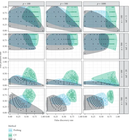
The results of the simulations for all settings are illustrated in Figure 1. With TPR and FDR on the𝑦-axis and𝑥-axis, respectively, solutions displayed in the top left corner of the plots therefore successfully separate𝑝infinformative variables from the ones without true effect on the response. Although already using a sparse cross-validation approach, the FDR of variable selection via cross-validation is still relatively high, with more than 50% false positives in the selected sets in the majority of the simulated scenarios. Whereas this seems to be mostly disadvantageous in the cases where𝑝inf = 5, the trend to more greedy solutions leads to a considerably higher chance of identifying more of the truly informative variables if𝑝inf = 20or with very high𝑝, however, still at the price of picking up many noise variables on the way. Pooling the results of all configurations considered for stability selection, the results cover a large area of the performance space in Figure 1, thereby probably indicating high sensitivity on the decisions regarding the three tuning parameters.
Examining the results separately in Figure 2, the dilemma is particularly clearly illustrated for 𝑝inf = 20and 𝑛 =
500. Despite being able to control the upper bounds for expected false positive selections, only a minority of the true effects are selected if the PFER is set too conservative. In addition, the high variance of the FDR observed for these configurations in some settings somewhat counteracts the goal to achieve more certainty about the selected variables one might probably pursue by setting the PFER very low. The performance of probing, on the other hand, reveals a much more stable pattern and outperforms stability selection in the difficult𝑝inf = 20and𝑛 = 100settings. In fact, the TPR is either higher or similar to all configurations used for stability selection, but exhibiting slightly higher FDR especially in settings with𝑛 = 500. Interestingly, probing seems to provide results similar to those of stability selection with PFER = 8, raising the question if the use of shadow variables allows statements about the number of expected false positives in the selected variable set.
Considering the runtime, however, we can see that prob-ing is orders of magnitudes faster with an average runtime of less than a second compared to 12 seconds for cross-validation and almost one minute for stability selection.
4. Application on Gene Expression Data
In this section we exploit the usage of probing as a tool for variable selection on three gene expression data sets. More specifically, this includes data from using oligonucleotide arrays for colon cancer detection [30] with40 tumor and
22 regular colon tissue samples and𝑝 = 2000measured genes expression levels. In addition, we analyse data from a study aiming to predict metastasis of breast carcinoma [31], where patients were labelled good or poor (𝑛 = 111
and𝑛 = 57, resp.) depending on whether they remained event-free for a five-year period after diagnosis or not. The data set contains log-transformed expression levels of𝑝 =
Probing CV SS 0.00 0.25 0.50 0.75 1.00 0.00 0.25 0.50 0.75 1.00 0.00 0.25 0.50 0.75 1.00 0.00 0.25 0.50 0.75 1.00 0.00 0.25 0.50 0.75 1.00 0.00 0.25 0.50 0.75 1.00 0.00 0.25 0.50 0.75 1.00
False discovery rate
T rue p o si ti ve ra te Method p = 1000 p = 500 p = 100 n = 100 n= 50 0 n = 100 n= 50 0 CH@ = 20 CH@ = 20 CH@ = 5 CH@ = 5
Figure 1: True positive rate (on𝑦-axis) and false discovery rate (on𝑥-axis) for three different, boosting-based variable selection algorithms, probing (black), stability selection (green), cross-validation (blue), and different simulation settings:𝑛 ∈ {100, 500},𝑝 ∈ {100, 500, 1000}, and
𝑝inf∈ {5, 20}. All settings of stability selection are combined. Shaded areas are smooth hulls around all observed values.
2905genes. The last example examines riboflavin production byBacillus subtilis[32] with𝑛 = 71observations of log-transformed riboflavin production rates and expression level for𝑝 = 4088genes. All data are publicly available viaR
packagesdatamicroarrayandhdi. Our proposed probing approach is implemented in a fork of the mboost [33] software for component-wise gradient boosting. It can be easily used by settingprobe=TRUEin theglmboost()call.
In order to evaluate the results provided by the new approach, we analysed the data using cross-validation, sta-bility selection [34], and the lasso [35] for comparison. Table 1 shows the total number of variables selected by each
method along with the size of the intersection between the sets. Starting with the probably least surprising result, boosting with cross-validation leads to the largest set of selected variables in all examples, whereas using probing as stopping criterion instead clearly reduces these sets. Since both approaches are based on the same regularization profile until the first shadow variable enters the model, the less regularized solution of cross-validation always contains all variables selected with probing. For stability selection, we used the conservative approach with PFER= 1and𝑞 = 20as suggested by B¨uhlmann et al. (2014) [32]. As a consequence, the set of variables considered to be informative further
6 Computational and Mathematical Methods in Medicine
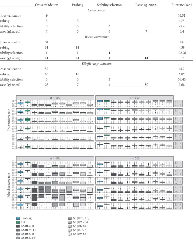
Table 1: Total number of selected variables and intersection size for four variable selection techniques (boosting with 25-fold bootstrap, probing, stability selection, and the lasso with 10-fold cross-validation) on three gene expression data sets. The last column compares algorithm runtime in seconds.
Cross-validation Probing Stability selection Lasso (glmnet) Runtime (sec.)
Colon cancer Cross-validation 9 10.52 Probing 5 5 1.78 Stability selection 3 3 3 49.4 Lasso (glmnet) 7 5 3 7 0.4 Breast carcinoma Cross-validation 32 24 Probing 14 14 4.39 Stability selection 1 1 1 102.28 Lasso (glmnet) 14 14 1 14 1.13 Riboflavin production Cross-validation 50 14.2 Probing 10 10 6.89 Stability selection 5 5 5 66.46 Lasso (glmnet) 23 7 4 30 0.68 0.00 0.25 0.50 0.75 1.00 0.00 0.25 0.50 0.75 1.00 0.00 0.25 0.50 0.75 0.00 0.25 0.50 0.75 0.00 0.25 0.50 0.75 T rue p o si ti ve ra te 0.00 0.25 0.50 0.75 1.00 0.00 0.25 0.50 0.75 1.00 0.00 0.25 0.50 0.75 1.00 0.00 0.25 0.50 0.75 1.00 0.00 0.25 0.50 0.75 1.00 0.00 0.25 0.50 0.75 1.00 F als e dis co ver y ra te Probing CV SS (0.6, 1) SS (0.75, 1) SS (0.9, 1) SS (0.6, 2.5) SS (0.75, 2.5) SS (0.9, 2.5) SS (0.6, 8) SS (0.75, 8) SS (0.9, 8) p = 1000 p = 100 p= 50 0 p = 1000 p = 100 p= 50 0 CH@ = 20 CH@ = 20 CH@ = 20 CH@ = 5 CH@ = 5 CH@ = 5 p = 1000 p = 100 p= 50 0 p = 1000 p = 100 p= 50 0 CH@ = 20 CH@ = 20 CH@ = 20 CH@ = 5 CH@ = 5 CH@ = 5 n = 100 n = 500 n = 100 n = 500 0.00 0.25 0.50 0.75 1.00
Figure 2: Boxplots of true positive rate (top) and false discovery rate (bottom) for different simulation settings and the three boosting-based, variable selection algorithms. Different Stability selection settings are denoted by SS(𝜋thr,PFER).
shrinks in all three scenarios. Again, these results clearly reflect the findings from the simulation study in Section 3, placing the probing approach between stability selection with probably overly conservative error bound and the greedy selection with cross-validation.
Since so far all approaches rely on boosting algorithms, we additionally considered variable selection with the lasso. We used the default settings of the glmnet package for R to calculate the lasso regularization path and determine the final model via 10-fold cross-validation [35]. Although the lasso already tends to result in sparser models under these conditions compared to model-based boosting [22],
glmnet additionally uses a “one-standard-error rule” to regularize the solution even further. In fact, this leads to the selection of an identical set of genes as probing for the breast carcinoma example, but the final models estimated for both other examples still contain a higher number of variables. This is especially the case for the data on riboflavin production, where the lasso solution is further not simply a subset of the cross-validated boosting approach and only agrees on 23 mutually selected variables. Interestingly, even one of the 5 variables proposed by stability selection is also missing. TheRcode used for this analysis can be found in the Supplementary Material of this manuscript available online at https://doi.org/10.1155/2017/1421409.
5. Conclusion
We proposed a new approach to determine the optimal number of iterations for sparse and fast variable selection with model-based boosting via the addition of probes or shadow variables (probing). We were able to demonstrate via a simulation study and the analysis of gene expression data that our approach is both a feasible and convenient strategy for variable selection in high-dimensional settings. In contrast to common tuning procedures for model-based boosting which rely on resampling or cross-validation procedures to optimize the prediction accuracy [21], our probing approach directly addresses the variable selection properties of the algorithm. As a result, it substantially reduces the high number of false discoveries that arise with standard procedures [14] while only requiring a single model fit to obtain the set of parameters.
Aside from the very short runtime, another attractive feature of probing is that no additional tuning parameters have to be specified to run the algorithm. While this greatly increases its ease of use, there is, of course, a trade-off regarding flexibility, as the lack of tuning parameters means that there is no way to steer the results towards more or less conservative solutions. However, a corresponding tuning approach in the context of probing could be to allow a certain amount of selected probes in the model before deciding to stop the algorithm (cf. Guyon and Elisseeff, 2003 [15]). Although variables selected after the first probe can be labelled informative less convincingly, this resembles the uncertainty that comes with specifying higher values for the error bound of stability selection.
A potential drawback of our approach is that due to the stochasticity of the permutations, there is no deterministic
solution and the selected set might slightly vary after rerun-ning the algorithm. In order to stabilize results, probing could also be used combined with resampling to determine the optimal stopping iteration for the algorithm by running the procedure on several bootstrap samples first. Of course, this requires the computation of multiple models and therefore again increases the runtime of the whole selection procedure. Another promising extension could be a combination with stability selection. With each model stopping at the first shadow variable, only the selection threshold𝜋thrhas to be specified. However, since this means a fundamental change of the original procedure, further research on this topic is necessary to better assess how this could affect the resulting error bound.
While in this work we focused on gradient boosting for binary and continuous data, there is no reason why our results should not also carry over to other regression settings or related statistical boosting algorithms as likelihood-based boosting [36]. Likelihood-based boosting follows the same principle idea but uses different updates, coinciding with gradient boosting in case of Gaussian responses [37]. Further research is also warranted on extending our approach to mul-tidimensional boosting algorithms [25, 38], where variables have to be selected for various models simultaneously.
In addition, probing as a tuning scheme could be gen-erally also combined with similar regularized regression approaches like the lasso [5, 22]. Our proposal for model-based boosting hence could be a starting point for a new way of tuning algorithmic models for high-dimensional data, not with the focus on prediction accuracy, but addressing directly the desired variable selection properties.
Conflicts of Interest
The authors declare that they have no conflicts of interest.
Acknowledgments
The work of authors Tobias Hepp and Andreas Mayr was sup-ported by the Interdisciplinary Center for Clinical Research (IZKF) of the Friedrich-Alexander-University Erlangen-N¨urnberg (Project J49). The authors additionally acknowl-edge support by Deutsche Forschungsgemeinschaft and Friedrich-Alexander-Universit¨at Erlangen-N¨urnberg (FAU) within the funding programme Open Access Publishing.
References
[1] R. Romero, J. Espinoza, F. Gotsch et al., “The use of high-dimensional biology (genomics, transcriptomics, proteomics, and metabolomics) to understand the preterm parturition syndrome,”BJOG: An International Journal of Obstetrics and Gynaecology, vol. 113, no. s3, pp. 118–135, 2006.
[2] R. Clarke, H. W. Ressom, A. Wang et al., “The properties of high-dimensional data spaces: implications for exploring gene and protein expression data,”Nature Reviews Cancer, vol. 8, no. 1, pp. 37–49, 2008.
[3] P. Mallick and B. Kuster, “Proteomics: a pragmatic perspective,”