Probabilistic topic modeling with latent Dirichlet allocation on Apache Spark

(1)

Treball final de grau

GRAU D’ENGINYERIA INFORMÀTICA

Facultat de Matemàtiques

Universitat de Barcelona

Probabilistic Topic Modeling with

Latent Dirichlet Allocation on

Apache Spark

Autor: Carlos Omar Cortés Hinojosa

Director:

Dr. Jesús Cerquides Bueno.

Co-director: Joan Capdevila Pujol.

Realitzat a:

Departament de matemàtica aplicada i anàlisi.

Barcelona,

30 de juny de 2016

(2)

Abstract

In a world in which we have access to vast amount of data, it is important to develop new tools that allow us to navigate through it. Probabilistic topic models are statistical methods to analyse text corpora and discover themes that best explain its documents. In this work, we introduce probabilistic topic models with special focus on one of the most common models called Latent Dirichlet Allocation (LDA). To learn LDA model from data, we present two variational inference algorithms for batch and online learning. Both algo-rithms are implemented on a popular Big Data computing framework known as Apache Spark. We introduce this framework and We study the algorithm scalability and topic co-herence in two different news data sets from New York Times and BBC News. The results point out to the need to tune up Apache Spark in order to boost its performance and to the goodness of the resulting topics in the BBC News dataset.

keywords: Probabilistic Topic Models, Latent Dirichlet Allocation, Apache Spark.

Resumen

En un mundo en el que tenemos acceso a gran cantidad de información, es impor-tante desarrollar nuevas herramientas que nos permitan navegarla. LosProbabilistic Topic Modelsson métodos estadísticos que analizan corpus de documentos y desvelan los temas que mejor explica sus documentos. En este trabajo presentamos los Probabilistic Topic Models con énfasis especial en uno de modelos más comunes llamado Latent Dirichlet Allocation (LDA). Para aprender el model LDA a partir del corpus, presentamos dos al-goritmos de inferencia variacional para aprendizaje por lotes y online. Ambos alal-goritmos están implementados en Apache Spark, un popular f rameworkBig Data. Introduciremos este framework y estudiaremos la escalabilidad de los algoritmos y la consistencia de los temas en dos conjuntos de notícias provenientes del New York Times y de BBC News. Los resultados señalan la necesidad de ajustar Apache Spark para incrementar el rendimiento y la buena calidad de los temas obtenidos en el conjunto de notícias de BBC News.

Palabras clave: Probabilistic Topic Models, Latent Dirichlet Allocation, Apache Spark.

Resum

En un món on tenim accés a una gran quantitat d’informació és important desenvolu-par noves eines que ens permetin navegar-la. Els Probabilistic Topic Modelssón mètodes estadístics que analitzen corpus de documents i rebel·len els temes que millor expliquen aquests documents. En aquest treball presentem els Probabilistic Topic Models amb es-pecial èmfasi en un dels algoritmes més comuns anomenat Latent Dirichlet Allocation

(LDA). Per aprendre el model a partir del corpus, presentem dos algoritmes de inf`rencia variacional per aprenentatge per lots i online. Ambdós algoritmes estan implementats en Apache Spark, un popular f ramework Big Data. Introduïrem aquest framework i estu-diarem l’escalabilitat dels algoritmes i la qualitat dels temes en dos conjunts de notícies provinents del New York Times i de BBC News. Els resultats apunten a la necessitat d’a-justar Apache Spark per incrementar el rendiment i la bona qualitat dels temes obtinguts en el conjunt de notícies de BBC News.

(3)

(4)

List of Figures

1.1 Example of the idea we talked about of exploring the data by topic applied

to the wikipedia articles. . . 2

1.2 The intuitions behind Latent Dirichlet Allocation. . . 4

1.3 Example of a graphical model and the usage of plates. . . 8

2.1 Graphical model for the Unigram Model. . . 10

2.2 Graphical model for the Mixture of Unigrams Model. . . 10

2.3 Graphical model for the Probabilistic latent Semantic Indexing Model. . . 11

2.4 Graphical model for the Latent Dirichlet Allocation. . . 12

2.5 Graphical model of the variational distribution. . . 13

2.6 Graphical model for the Smoothed Latent Dirichlet Allocation. . . 16

3.1 Different phases of performing a word count with the MapReduce framework. 20 3.2 Components of Spark. . . 21

3.3 Most commons operations available on RDDs in Spark. . . 23

3.4 Spark architecture. . . 24

3.5 Flow of the example application with a sample dataset and DAG generated. 25 3.6 Hash-based Shuffle. . . 27

3.7 Sort-based Shuffle. . . 27

4.1 Scheme of the (virtual) architecture used during the testing. . . 30

4.2 Line chart for the results with EM optimizer. . . 34 iii

(7)

iv

4.3 Line chart for the median of the execution time of the attempts with the em optimizer and the locality parameter configured to wait vs the attempts without it. . . 35 4.4 Line chart for the execution time for each attempt with the online optimizer. 35

(8)

Chapter 1

Introduction

1.1 Introduction and motivation

Historically, when looking for a specific piece of information, like a scientific article or a news piece, the main problem was gaining access to such information. Today we have instant access to as much data as we could wish for thanks to the Internet, and that has become a problem on its own. Our two main tools to navigate through all the online information nowadays are searches and links. From a few keywords a search engine sends us to some documents related to those keywords where we find links to other related documents.

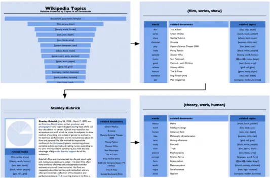
Although we may think this is a powerful way of working with the data and likely the only we can think of, something is missing. It would be really useful if we were able to explore the data or documents based in its theme. Most of the time we are looking for information about a topic or a subject instead of a keyword. So rather than finding documents through keyword searches alone, imagine being able to search and explore documents based on themes that run through them. We might “zoom in” or “zoom out” to find specific or broader themes or even look at how themes changed through time or how they are connected to each other. It is also worth pointing out that knowing the themes of the documents can also improve the accuracy of the search and it is safe to assume that search engines already use Topic Modeling to some extent, we are just introducing a use case for the set of techniques we will explain and use along this work. Figure 1.1 shows one application of the topic-based navigation we talked about.

Topic models provide a way of making possible the situation we talked about. We will give a more detailed and rigorous definition in the following chapter but from a high level point of view we can define Topic Modeling as a way of identifying hidden patterns in a corpus1. For example by assigning a set of topics to each document of the collection. We will need to define what we understand for a topic, but for now we can think as the themes the document talks about. The topics we obtain with a Topic Modeling algorithm can be used for example to summarize, visualize and explore the corpus.

Throughout this work we will focus on the most common Topic Modeling algorithm called Latent Dirichlet Allocation (LDA for short). In broad terms, LDA is an

unsuper-1_{Large collection of documents.}

(9)

2 Introduction vised generative model that tries to capture the intuition that each document exhibits multiples topics.

One of the main challenges of Topic Modeling is dealing with large amounts of infor-mation since for a small amount of documents it is easier to just read and study each one of the documents. That forces us to be aware of the amount of computation power it will need and that is why will analyze how LDA works and scales in a big data ecosystem like Apache Spark.

Figure 1.1: Example of the idea we talked about of exploring the data by topic applied to the wikipedia articles. (Source: http://www.princeton.edu/~achaney/tmve/wiki100k/ browse/topic-presence.html)

1.2 Objectives and organization

This work revolves around two main concepts, Latent Dirichlet Allocation and Apache Spark and the main objectives of this project are to understand and work with those two concepts.

The first main objective of this work is to introduce the concept of Probabilistic Topic Models and present one of the main algorithms in this field called Latent Dirichlet Alloca-tion from a theoretical point of view with two algorithms for the inference process: Batch Variational Bayes and Online Variational Bayes.

As we commented in the previous section, one of the main challenges of Topic Mod-eling is dealing with large amounts of data so the second main goal of this project is to make use of the Latent Dirichlet Allocation and analyze how it performs and scales in a big data context. Apache Spark plays a big factor in this part so we will need to get a deep understanding of how it works in order to make sense of the performance results we get. For this part we needed a big text dataset, and that is not always easy to find, we

(10)

1.2 Objectives and organization 3 will use a dataset made of news articles from the New York Times2 that comes already preprocessed as a bag of words and is big enough to allow us analyze the performance.

Lastly, after seeing how it performs and scales we want to show how the results of the Latent Dirichlet Allocation are. By that we mean the topics it finds on the corpus and the topics it assigns to each article. The articles from the New York Times dataset are not available with the dataset, we only have a word count, so we decided to use a second dataset where we have the articles. This dataset is from the BBC3 and already comes divided in five topics: business, entertainment, politics, sports and tech. This will also help us see how well LDA finds the topics.

According to the objectives this work is organized as follows:

• In Chapter 1 we introduce the work, the objectives and some previous concepts we will need later on.

• In Chapter 2 we review Probabilistic Topic Models with special focus in LDA and the two inference algorithms (Batch Variational Bayes and Online Variational Bayes). • In Chapter 3 we introduce Apache Spark, explain how it works and all the concepts

needed to understand the performance results of Chapter 4.

• In Chapter 4 we test the performance and evaluate the scalability of the LDA imple-mentation in Apache Spark with the New York Times dataset. In the last part of the chapter we show a real word application of LDA using Spark with the BBC news dataset.

Now we will intuitively introduce the two main concepts we previously said: Latent Dirichlet Allocation and Apache Spark.

1.2.1 Latent Dirichlet Allocation

Latent Dirchlet Allocation is a generative model, that means that the algorithm aims to generate a probabilistic model for randomly generating the data. It is easier to under-stand the idea of a generative model with an example: imagine that we want to learn to distinguish between dogs and cats based on some features of the animal.

One possible approach would be to observe a lot of dogs and cats, that would be our training set, and try to deduce a decision boundary from those observations. This would be the approach used by discriminative algorithms. Instead, a generative algorithm would try to build a model of what dogs look like by looking at dogs and then, by looking at cats, a model of what cats look like. Then to classify a new animal all we need to do is check which one of the two models is more likely to generate the new animal.

The model LDA generates it is not about cats and dogs obviously, it is about docu-ments. The basic idea to generate a document in LDA is as follows:

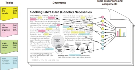
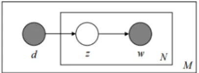
• We assume we have a number of topics that exists for the whole collection of docu-ments (left side of Figure 1.2).

2_{Available in [1]} 3_{Available in [2]}

(11)

4 Introduction • Randomly select a mixture of topics for the document (the histogram at the right of Figure 1.2). We are assuming we have a number of topics that exists for the whole collection of documents (left side of Figure 1.2).

• For each word in the document we draw a topic from the mixture. Conditioned to the topic, we draw a word (the colored coins of Figure 1.2).

Figure 1.2: The intuitions behind Latent Dirichlet Allocation. All the data shown is only illustrative.

Source:https://www.cs.princeton.edu/~blei/papers/Blei2012.pdf.

Of course this generated document will not make any sense to a human, that is not the purpose of the algorithm anyway, we are interested on the way this model can help us gain insights from the document collection. We will see how it does in that regard in Chapter 4.

1.2.2 Apache Spark

Apache Spark is an open source project originally developed at the University of Cal-ifornia, Berkeley, in 2009 and currently maintained by the Apache Software Foundation. We previously referred to Spark as a big data environment but more precisely it is a cluster computing framework built around speed, ease of use and sophisticated analytics. It can run in Hadoop clusters through YARN or Spark’s standalone mode4, and it can process data in HDFS, HBase, Cassandra, Hive, and any Hadoop InputFormat. It is designed to cover a wide range of workloads including batch processing (similar to Hadoop’s MapRe-duce) and new workloads like streaming, interactive queries, and machine learning. Spark is written and built in Scala, that explains why we have chosen Scala for this project, but it contains APIs for Python, Java and R.

The experimental part of this project has been developed in Spark 1.5.1 that was re-leased in October 2, 2015. Current version as of June 2016 is 1.6.1 where no noticeable changes were done as far as this project concerns.

(12)

1.3 Planning 5

1.3 Planning

This work is worth 18 ECTS credits and each credit corresponds to 25 work hours. So, this work is equivalent to 450 work hours. The usual span of a project like this is one semester (around 20 weeks), but since I was working full-time during the realization of this project it took two semester (around 40 weeks) to finish it.

1.4 Notation and terminology

During this work we will use the same terminology used by David Blei in the 2003 article where he presented the Latent Dirichlet Allocation5so we will use the language of text collections. Formally, we define the following terms:

• A word is the basic unit of discrete data, defined to be an item from a vocabulary indexed by{1, ...,V}. We represent words using unit-basis vectors that have a single component equal to one and all other components equal to zero. Thus, using super-scripts to denote components, thev-th word in the vocabulary is represented by a by aV-vectorwsuch thatwv=1 andwu=0 foru6=v.

• A document is a sequence ofNwords denoted byw= (w1,w2, ...,wN), wherewnis then-th word in the sequence.

• A corpus is a collection ofMdocuments denoted byD=w1,w2, ...,wM.

1.4.1 Some Probability Concepts

Prior and posterior distributions

When introducing the Latent Dirichlet Allocation in chapter 2, we will be using the termspriorandposteriorprobabilities andlikelihoodfunction:

• The prior probability distribution of and uncertain quantity is the probability dis-tribution that express the value of this quantity before some evidence is taken into account.

• The posterior probability is the conditional probability after some evidence is taken into account.

• The likelihood function of a set of parameters given some outcome is equal to the probability of observing said outcome given those parameter values.

If the prior and the posterior distributions are in the same distribution family, then the prior and posterior are calledconjugate distributions and the prior is called a conjugate prior for the likelihood funtion.

(13)

6 Introduction Given a prior p(θ) and observations x with the likelihood p(x | θ), the posterior is

defined as:

p(θ|x) = p(x|θ)p(θ)

p(x)

Jensen Inequality

In the context of probabilities, the Jensen Inequality is stated as follows: If X is a random variable and f a convex function then:

f(E[X])≤E[f(X)]

And, if f is a concave function the inequality turns:

f(E[X])≥E[f(X)]

Kullback-Leibler (KL) divergence

When formulating the optimization problem in Latent Dirichlet Allocation we will use the KL divergence to express the optimization problem. The KL divergence is a measure of the difference between two probability distributionsP and Q. It is important to note that the KL divergence is not symmetrical inPandQso it’s not a metric.

The KL divergence can be interpreted as a way to express the amount of information lost whenQis used to approximateP6

Given two continuous distributionsPandQthe KL divergence is defined as follows:

DKL(P||Q) =

Z +∞

−∞ p(x)log

p(x)

q(x)dx

This can also be expressed using the definition of expectation (and expressing the log of a division as difference of log) as:

DKL(P||Q) =Ep[log p(x)]−Ep[log q(x)] This is the expression we will use later on instead of the definition.

We present now the two probability distributions we will be using when we define the different models in this work: the Multinomial and the Dirichlet distributions. Multino-mial Distribution

The multinomial distribution models the histogram of outcomes of an experiment with

kpossible outcomes that is performedntimes. The parameters of this distribution are the

6_{This is a quote from the book Model Selection and Multi-Model Inference by K.P. Burnham and D.R.}

(14)

1.4 Notation and terminology 7 probabilities of each of thekpossible outcomes occurring in a single trial, p1, ...,pk. This is a discrete, multi-variate distribution with probability mass function:

f(x1, . . . ,xk|n,p1, . . . ,pk) =Pr(X1=x1and . . . andXk=xk) = =          n! x1!· · ·xk! px1 1 · · ·p xk k , when ∑ k i=1xi =n 0 otherwise

A good example of how the multinomial distribution is used is to think of rolling a dice several times. Say you want to know the probability of rolling 3 fours, 2 sixes, and 4 ones in 9 total rolls given that you know the probability of landing on each side of the dice. The multinomial distribution models this probability.

For LDA we will use a Multinomial Distribution with n = 1 that is also known as Categorical Distribution that simplifies the probability mass function to:

f(x1, . . . ,xk| p1, . . . ,pk) = k

∏

i=1 pxi i Dirichlet Distribution

As we can guess by its name, we will be using this distribution when we explain the Latent Dirichlet Allocation. The Dirichlet distribution is a bit tricky to understand because it deals with distributions over the probability simplex. This means that the Dirichlet distribution is a distribution over discrete probability distributions. Its probability mass function is (maintaining the notation introduced for the Multinomial definition):

P(P={pi}|αi) = ∏iΓ

(αi) Γ(_∑iαi)

∏

_i

pαi−1

i

Whereα= (α1,· · ·,αk)with αi >0 for eachi is the parameter of the Dirichlet distri-bution.

The key to understanding the Dirichlet distribution is realizing that instead of it being a distribution over events or counts (as most common probability distributions are), it is a distribution over discrete probability distributions (eg. multinomials).

The reason why we use the Dirichlet Distribution in Latent Dirichlet Allocation is that we will model the topics as multinomials and the Dirichlet Distribution is the conjugate prior of the multinomial which facilitates the development of the algorithm.

We call exchangeable Dirichlet Distribution with a single scalar parameter η to a

(15)

8 Introduction

1.4.2 Graphical Model

Graphical models are a way to encode the conditional dependence structure between random variables of probabilistic models in a visual way (in a directed graph):

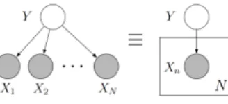
• Nodes represent random variables. • Edges denote possible dependence. • Shaded variables are shaded nodes. • Plates represent replicated structure.

For example the following figure shows an example of a graphical model. The edge between X1 and Y means that X1 depends onY. The shaded nodes X1, ..., Xn means that they are observed variables. Y is a hidden or latent variable. The plate denote the replicated structure.

Figure 1.3: Example of a graphical model and the usage of plates.

The structure of the graph defines the pattern of conditional dependence between the random variables. From the graph in the figure we can derive the joint probability distribution: p(Y,X1,· · ·,Xn) =p(Y) N

∏

n=1 p(Xn|Y)

(16)

Chapter 2

Probabilistic Topic Models

2.1 Background

We already talked a bit about this concept in the introduction but we have not defined the concept of Probabilistic Topic Model yet. From Blei 2012 "Probabilistic Topic modeling algorithms are statistical methods that analyze the words of the original texts to discover the themes that run through them." In section 1.1.1 we introduced an example of a Prob-abilistic Topic Model. We will present it again in this chapter along with all the details we ignored in the introduction. But before that we will review some significant progress made in this field before LDA.

In the following sections we use the notation introduced in section 1.4 wherewdenotes a document,wn denotes then-th word of the document andNdenotes the length of the document.

2.1.1 Unigram Model

1

The most simple Probabilistic Topic Model we are going to talk about is the Unigram Model. In this model the words of every document are generated independently from a single multinomial distribution. So the probability of a document is the product of the probability of each of the words:

p(w) =

N

∏

n=1

p(wn)

We can illustrate the model by the graphical model in figure 2.1.

1_{More detail about the Unigram Model as well as the generalization to the n-gram model can be found in [3]}

(17)

10 Probabilistic Topic Models

Figure 2.1: Graphical model for the Unigram Model.

2.1.2 Mixture of Unigrams

2

This model adds a discrete random variablez to the Unigram Model that represents the topic of the documents. To generate a document under this model we select a topic

zfor the document and then select the words from the conditional Multinomial p(w|z). So the probability of a document is the sum of the probability of choosing the topic z

represented as p(z) and then drawing the N words independently conditioned by the chosen topic, that isp(w|z):

p(w) =

∑

z p(z) N

∏

n=1 p(wn|z)

The mixture of Unigrams Model is represented by the following graphical model (Fig-ure 2.2):

Figure 2.2: Graphical model for the Mixture of Unigrams Model.

When we generate this model from observations of a corpus we can consider the words distributions p(w|z) as representations of topics assuming that each documents is about a single topic. We will face this issue in LDA by introducing one more parameter to the model.

2.1.3 Probabilistic latent Semantic Indexing (PLSI)

3

PLSI attempts to solve the issue of having only one topic per document. PLSI proposes that a document label d and a wordwn are conditionally independent given and unob-served topicz. And by adding this we are allowing a document to have multiple topics, the topic weights of a documents are represented byp(z|d).

p(d,wn) =p(d)

∑

z

p(wn|z)p(z|d)

2_{In depth article about the mixture of unigram model can be found in [4]} 3_{Original article can be found in [5]}

(18)

2.2 Latent Dirichlet Allocation 11 Here,donly acts as index to the document in the collection.dis a Multinomial random variable with as many possible values as the size of the training documents and the model learns the topic weights,p(z|d), only for those documents on which it is trained sinced

is the index of the document in the collection. That makes it hard to assign to new unseen documents and makes the model prone to overfitting the training set.

The PLSI Model can be represented by the following graphical model (Figure 2.3):

Figure 2.3: Graphical model for the Probabilistic latent Semantic Indexing Model.

2.2 Latent Dirichlet Allocation

In this section we will be following the original article where the Latent Dirichlet Allocation4. Our main goals here are to understand the LDA model and understand the setting of the algorithm and how we transform the inference problem to an optimization problem. We consider the notation introduced section 1.3.

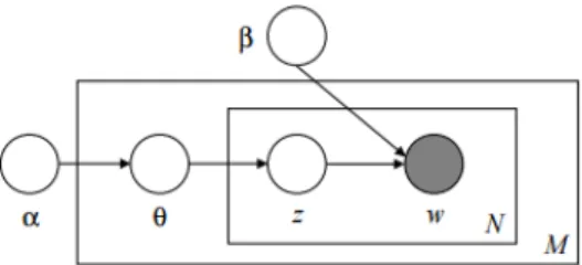
We have already introduced the Latent Dirichlet Allocation as a generative probabilistic model of a corpus of text documents and presented in an intuitive manner the generative process. We will give now a more rigorous and in-depth explanation. Documents are represented as mixtures over latent topics and each topic is characterized by a distribution over words. LDA assumes the following generative process for each document:

1. ChooseN∼Poison(ξ). This will represent the length of the document.

2. Chooseθ∼Dir(α). This will represent the mixture of topics for the document.

3. For each of theNwordswn:

(a) Choose a topiczn∼Multinomial(θ). The topic we choosewn from.

(b) Choose a word wn from p(wn | zn,β), a multinomial probability conditioned

on the topiczn.

First we observe that the model assumes that the document length,N, is independent of the data generating variables (θ and z) so the Poisson can be changed for another

distribution that generates more realistic lengths of documents. In this model we are assuming that the dimensionalityk of the Dirichlet distribution is fixed. In practice this will mean that we fix the number of topics before executing the algorithm. The word probabilities are parameterized by ak×V matrixβwhere βi,j = p(wj = 1,zi =1)is the probability of the word jof the vocabulary in the topici . For now, we can think ofβas

a fixed quantity that needs to be estimated. θin this model represents the probability of

each topic for the document.

(19)

Figure 2.4: Graphical model for the Latent Dirichlet Allocation.

Figure 2.4 shows the probabilistic graphical model for LDA. We can see that there is three level of parameters in LDA, α and β that are corpus-level parameters. θ is a

document-level parameter sampled once per document. And finally,z andw are word-level variables and are sampled once for each word in each document.

Given the parameters αand β, the joint distribution of a topic mixture θ, a set of N

topicsz, and a set ofNwordsw(a document) is given by:

p(θ,z,w|α,β) =p(θ|α)

N

∏

n=1

p(zn |θ)p(wn |zn,β) (2.1)

Observe that p(zn |θ), the probability of choosing the topicngiven a topic mixtureθ,

isθi for the uniqueithat corresponds to the topiczn. To obtain the marginal distribution of a document we integrate overθand sum overz:

p(w|α,β) = Z p(θ|α) N

∏

n=1

∑

zn p(zn|θ)p(wn|zn,β) dθ (2.2)

If we want to obtain the probability of a corpus we just need to take the product of the marginal probabilities of single documents:

p(D|α,β) = D

∏

d=1 Z p(θ_d|α) Nd

∏

n=1

∑

zdn p(zdn |θd)p(wdn|zdn,β) dθ_d

As we earlier commented, the goal of the Latent Dirichlet Allocation is not to generate documents or corpus. The corpus is already generated, what we want is to gain informa-tion about the topics of the documents. That brings us our main inference problem, we are interested on computing the posterior probability of the variables θ and zgiven the

datawand the hyperparametersαandβ.

p(θ,z|w,α,β) = p(θ,z,w|α,β)

p(w|α,β) (2.3)

See (2.1) for the value of the numerator and (2.2) for the denominator of the posterior distribution (2.3). The computation of this denominator is intractable to compute in gen-eral because when we write equation 2.2 in terms of the model parameters we find an intractable coupling betweenθand β5. Since this distribution is intractable for exact

in-ference we need to use an approximate inin-ference algorithm. We will show two algorithms

(20)

2.3 Variational inference for LDA 13 for this purpose: Batch Variational Inference, the one introduced in the original article we’ve been following so far, and Online Variational Inference, introduced in 2010.

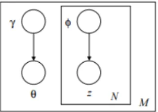
2.3 Variational inference for LDA

The intractability of the above equation 2.2 is due to the coupling between variables

θand β. The variational inference scheme considers a factorized variational distribution

which approximates the posterior distribution. This factorized variational distribution is expressed as follows: q(θ,z|γ,φ) =q(θ|γ) N

∏

n=1 q(zn |φn) (2.4)

Whereγand(φ1,· · ·,φN)are the free variational parameters. The resulting graphical model is shown in figure 2.5.

Figure 2.5: Graphical model of the variational distribution.

To determine the values of the variational parameters γ and (φ1,· · ·,φN)we set up an optimization problem. We want to maximize the log likelihood of a document which translates into an optimization problem. Now we show the process to obtain the opti-mization problem. logp(w|α,β)(1)= log Z

∑

z p(θ,z,w|α,β)dθ(2)= log Z

∑

(1) we marginalize overθandz.

(21)

14 Probabilistic Topic Models (3) we use the definition of expectation.

(4) we apply Jensen’s inequality ( f(E[X])≥E[f(x)]if f(E[X])is a convex function). (5) Apply the property of log function that says thatlogof the division is equal to the difference oflog’s.

(6) Since the expectation is a linear operator we can separate the twolog.

We obtained a lower bound for the logp(w | α,β) that we will denote for now on

as L(γ,φ | α,β). Now we are going to observe that the difference between the lower

bound we obtained and logp(w |α,β)is the KL divergence between p(θ,z| w,α,β)and

q(θ,z|γ,φ):

First we calculate the KL divergence between p(θ,z | w,α,β) and q(θ,z) using the

expression we deduced in the introduction:

DKL(q(θ,z|γ,φ)|| p(θ,z|w,α,β)) =E_q(_θ,z|γ,φ) h logq(θ,z|γ,φ) i −Eq(θ,z|γ,φ) h logp(θ,z|w,α,β) i

Adding the KL divergence with the lower bound we obtain:

DKL(q(θ,z|γ,φ)||p(θ,z|w,α,β)) +L(γ,φ|α,β) = Eq(θ,z|γ,φ) h logq(θ,z|γ,φ) i −E_q(_θ,z|γ,φ) h logp(θ,z|w,α,β) i +E_q(_θ,z|γ,φ) h logp(θ,z,w|α,β) i −Eq(θ,z|γ,φ) h logq(θ,z|γ,φ) i₍₇₎ = (7) = E_q(_θ_,z|_γ_,_φ₎hlogp(θ,z,w|α,β) p(θ,z|w,α,β) i₍₈₎ =E_q(_θ_,z|_γ_,_φ₎hlogp(w|α,β) i₍₉₎ = logp(w|α,β)

(7) We use that the expectation is linear and that difference of log’s is equal to the log of the division.

(8) Using equation (2.3).

(9)logp(w|α,β)does not depend on q.

So, as a function of the variational distribution, minimizing the KL divergence is the same as maximizing the ELBO. We obtained our optimization problem:

(γ∗,φ∗) =argmin₍_γ_,_φ₎DKL(q(θ,z|γ,φ)||p(θ,z|w,α,β))

This minimization can be achieved by a fixed point method6_{. This yields algorithm 1:} WhereΨis the first derivative of thelogΓfunction.

6_{We skip the calculations since they are particular to this application of Variational inference, all the details}

(22)

2.3 Variational inference for LDA 15 Algorithm 1Variational Inference for LDA

1: Initializeφ_ni0 :=1/kfor alliandn

2: Initializeγi:=αi+N/kfor alli 3: repeat 4: forn=1 toN 5: fori=1 to k 6: φt+1_ni :=βiwnexp(Ψ(γ t i)) 7: Normalizeφt+1_ni to sum 1 8: γt+1:=α+∑_n=1N φ_nit+1 9: untilconvergence Parameter Estimation

So far we have treated the model parametersαandβ as fixed quantities, when using

the algorithm for real world applications we want a way to estimate them. Given a corpus of D = {w1, ...,wM} documents, we want the values for αand βthat maximize the log

likelihood of the corpus:

`(α,β) =

M

∑

d=1

logp(wd|α,β)

We already commented on the fact that p(w|α,β)can not be computed, but we have

a lower bound on the log likelihood that can be maximized with respect toα and β. So

we can obtain estimates for the parameters via aVariational Expectation Maximization

procedure that can be summarized as follows:

• E-step: For each document, find the optimizing parameters {γ∗_d,φ∗_d : d ∈ D} as

described before.

• M-step: Maximize the resulting lower bound with respect to the model parameters

αandβ.

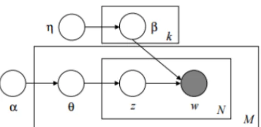
2.3.1 Smoothed LDA

7

Before we start explaining the the Online Variational Inference we need to present a slight modification to the LDA model we have shown in the previous section called the smoothed LDA. The smoothed LDA modifies the LDA model by treatingβas a random

matrix. Each row ofβ is drawn independently from an exchangeable Dirichlet with

pa-rameterη. The graphical model representation for this model is shown in figure 2.6. We

add theη hyperparameter because with the LDA model we estimateβassigning

proba-bility zero to all the words not found in any document of the training set used to build the model.

The inference process we showed in the previous section can be adapted to bear in mind the fact thatβis a randomk×Vmatrix (or equivalentlykvectors of lengthV), we

add a parameterλto the factorized variational distribution. We will not show the details

but a similar process to the one we have shown in the previous section the variational

(23)

Figure 2.6: Graphical model for the Smoothed Latent Dirichlet Allocation.

process can be adapted to the smoothed model and algorithm 1 remains the same with the addition of the update for the new parameterλwe introduced. The update equation

forλis: λij=η+ M

∑

d=1 Md

∑

n=1 φ_d∗ niw j dn

2.4 Online Variational Inference

8

Variational inference requires to pass through the whole dataset for each iteration, and that can be a problem when working with big datasets and is not an option to use cases where the data is arriving constantly. The Online Variational Inference algorithm aims to solve both problems without compromising the quality of the obtained topics and with an algorithm nearly as simple as Variational Inference. For this algorithm we will only highlight the differences respect the Variational Inference and the resulting algorithm. The key difference is the way to fit the variational parameterλrespect the Variational Inference

explained in the previous section.

As we observe thet-th document (or equivalently a vector of words counts) we perform the E-step like Variational inference9 to find locally optimal values for γt and φt while holding λ fixed. And then (the M-step) compute the optimal value for λ if the whole

document corpus consisted of thist-th document repeatedMtimes (remember that Mis the number of documents in the corpus). After we have the optimal value of λ for the

document, we call itλ∗, we update the value ofλusing a weighted average of its previous

value and λ∗_d. The weight given to λ∗ is given byρt = (τ0+t)−κ, with κ ∈ (0.5, 1]. κ

controls the importance we give to most recents values ofλ∗.

Algorithm 2 shows the inference process given a vector of word counts. The explicit formulas forEq[logθtk]andEq[logβkw]are:

Eq[logθ_tk] =Ψ(γ_tk)−Ψ( K

∑

i=1 γti) Eq[logβkw] =Ψ(λkw)−Ψ( W

∑

i=1 λki)

8_{Original article can be found in [8].}

(24)

2.4 Online Variational Inference 17 WhereΨdenotes de derivative of the logarithm of the gamma function.

Algorithm 2Online Variational Inference for smoothed LDA 1: Defineρt= (∆ τ0+t)−κ

2: Initializeλrandomly.

3: fort=0to∞do 4: E-Step:

5: Initializeγtk =1 (The constant 1 is arbritary.) 6: repeat

7: Setφtwk∝exp{Eq[logθtk] +Eq[logβkw]} 8: Setγtk=α+∑wφtwkntw 9: until _K1∑k |change inγtk|<0.00001 10: M-Step: 11: Computeλ∗_kw=η+Dntwφtwk 12: Setλ= (1−ρt)λ+ρtλ∗ 13: end for

The fact that we are updating all the parameters by only observing a single document allows us to use the algorithm in situations where the data is constantly arriving

(25)

(26)

Chapter 3

Apache Spark

We have already introduced Apache Spark in Chapter 1, in this chapter we will analyze in depth the Apache Spark ecosystem and its architecture but first we comment on the motivation behind Spark and the reasons behind the rise in popularity it is currently experimenting.

3.1 Motivation

Apache Sparks appears around 2009 as a response to the need for tools that adapted efficiently to new workloads ( e.g. interactive queries and machine learning ) since the options available at the time were not optimized for that1. The main tool available at the time was Hadoop’s MapReduce that it is a good solution for one-pass computations but not optimized for iterative workloads that are common in machine learning. In the MapReduce framework each step done while processing the data has one Map phase and one Reduce phase and you will need to convert any processing needs into MapReduce pattern to take advantage of this solution adding complexity to the process. In figure 3.1 we can see an example of MapReduce.

The concept behind MapReduce is divide the data in multiple parts and storing them in different machines in a cluster performing the operations on those machines (Mapping phase) and sending the results to another machine in the cluster (Reduce phase). The main performance drawback for iterative workloads comes from the fact that the data is stored and read from the disk in each step of processing and I/O from disk is really slow. Map step reads data from disk/hard drive, processes it and send it back to disk before performing shuffling operation to send data to reduce. At reduce, again reads data from disk, processes it and writes data back to disk. This is a major drawback performance-wise when multiple rounds of computations are performed on the same data. To overcome this limitation (while retaining the scalability and fault tolerance of MapReduce) Spark introduced the concept of Resilient Distributed Dataset (RDD) which are in-memory data structures that can be kept in memory across a set of nodes that can be rebuilt if a partition is lost.

1_{Explained by one of the main minds behind Spark in this interview from May 2015 available here:} _http: //www.kdnuggets.com/2015/05/interview-matei-zaharia-creator-apache-spark.html

(27)

20 Apache Spark

Figure 3.1: Different phases of performing a word count with the MapReduce framework.

Aside from the performance point of view this is another point where spark shines: the simplicity. As we said before, working with the MapReduce framework means adapting the computations to the MapReduce pattern. The programmer is required to think only in terms of basic operations of Map and Reduce. And the task of adapting every problem to this patter is not trivial. Common operations can require a significant amount of work. For example a simple word count program needs around 60 lines of code in Hadoop MapReduce while the same can be achieved in only one line in the interactive shell of Spark.

3.2 Spark Overview

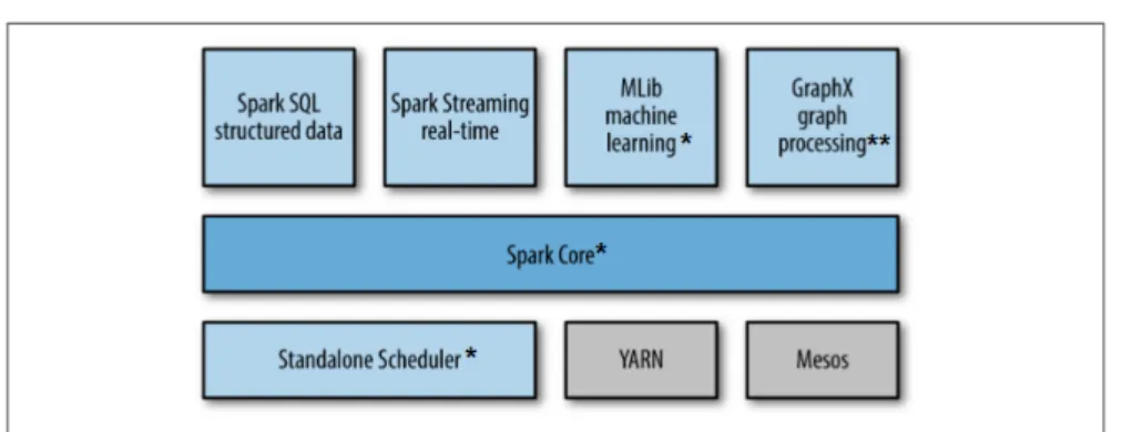
By the Spark project we are referring to a set of different components each one spe-cialized in different workloads. We can see the components in figure 3.2. At its core is a "computational engine" that is responsible for scheduling, distributing, and monitoring applications consisting of many computational tasks across acomputing cluster. This core engine powers multiple higher-level components.

This design philosophy comes with several benefits. The obvious one is that the higher level components benefit from any improvement done in the lower layers. Another ben-efit is the cost of running the stack is minimized, instead of running a few independent software systems only one it is needed. This reduces significantly the cost of trying new types of analysis inside an organization.

As shown in the figure 3.2 we will only be using a few components of the whole Spark stack but we will briefly introduce each one of them:

Spark SQL

This component provides a SQL interface to Spark, allowing developers to perform SQL queries and programmatic data manipulations in the same application. It is the main way for Spark to work with structured data.

Spark Streaming

(28)

3.2 Spark Overview 21

Figure 3.2: Components of Spark. Marked with * the components we actively used on this project. ** Is used for the implementation of theEMOptimizer of LDA.YARNandMesos

are not developed in the Spark project but appear on the picture because Spark can run on those two.

For example log files from a server or messages on social media. Under the hood, Spark Streaming retains the scalability and fault tolerance of the Spark Core.

MLib

MLib is Spark’s machine learning library. It provides multiple types of machine learn-ing algorithms, includlearn-ing classification, regression, clusterlearn-ing2among others. All of these algorithms are designed to scale out across a cluster. The Latent Dirichlet Allocation is implemented in this library as a part of the clustering algorithms.

GraphX

GraphX is a library for manipulating graphs and performing graph-parallel compu-tations. Extends the Spark RDD API providing operations to manipulate graphs and a library of common graphs algorithms.

Spark Core

We will review in depth this component in the following sections, since this component contains the basic functionality of Spark, including components for task scheduling , mem-ory management, fault recovery, interacting with storage systems, and more. Spark Core contains the main programming abstraction of Spark, the Resilient Distributed Datasets (RDDs).

Cluster Managers

Spark can run over a variety of cluster managers including Hadoop YARN and Apache Mesos. It also includes a simple cluster manager called the Standalone Scheduler. We will be using the Standalone Scheduler in the tests of chapter 4.

(29)

22 Apache Spark

3.3 Spark Programming Model

To use Spark the developer writes a driver program that controls the high-level flow of the application and launches operations in parallel (or calls to the API that launch operations). Each dataset is represented as an object and operations are invoked using methods on these objects. As part of the Spark Core component, the Spark API provides two main abstractions for the developer: theResilient Distributed Dataset(RDD) and the

parallel operations:

3.3.1 Resilient Distributed Dataset

A Resilient Distributed Dataset is a read-only collection of objects partitioned across the cluster that can be rebuilt if a partition is lost. RDDs can contain any type of Python, Java, or Scala objects, including user-defined classes. The most usual ways to create an RDD are:

• Load from a file with the built in functions from a shared file system. For example loading a text file from HDFS (Hadoop Distributed File System).

• Parallelize a collection (e.g. an array from Scala) in the driver program.

• Transform another RDD. Although RDDs are immutable, we can apply transforma-tions to an already existing RDD in order to create a new one that represents the new state of the previous RDD.

Most of the times when working with RDDs its elements do not exist in physical storage. An RDD only stores the information about how it was derived from others datasets so it can be computed at any time but it does not need to contain the computed data at all times. This allows the program to be able to reconstruct all the RDDs in case of failure.

The user can also control the persistence and the partitioning of an RDD. Persistence allows the developer to change if the RDD it is kept in memory so it can be reused faster in future operations. The partitioning controls how the dataset is spread across the cluster3. It is important to note that even if the persistence level is set to keep the RDD in memory it will spill to disk if there is not enough memory for it. It works this way so the system keeps working in case of failure of some nodes (or if a dataset is too big)4_.

As we commented before when talking about the motivation behind Spark, RDDs are best suited for batch applications where the same operation is done to all elements of a dataset since it can efficiently remember each transformation as one step. However this design makes RDDs less suitable for applications that make constant asynchronous updates like a storage system or a web crawler.

3_{We will comment more about how the partitioning affects real world performance and scalability in Chapter}

4.

4_{The user can also request other persistence strategies, like storing an RDD only on disk or duplicate it across}

(30)

3.4 Spark Architecture 23

3.3.2 Parallel Operations

There are two types of operations in Spark: transformations, that construct a new RDD from a previous one, and actions, that compute a result based on an RDD. The main dif-ference between transformations and actions comes from the way Spark computes RDDs. Although you can define new RDDs any time, transformations are computed in a lazy fashion, while actions launch a computation. Lazy fashion means that the transforma-tions are not computed until the first time the RDD is used in an action. This may not make sense at first but it allows to make optimizations before executing the job.

Figure 3.3: Most commons operations available on RDDs in Spark.5

3.4 Spark Architecture

In this section we will focus on the Spark Standalone Cluster that is the built-in cluster and comes with the default distribution. Most of the concepts are applicable for YARN and MESOS6but there may be some slight differences. Spark uses a master/slave architecture7 where the driver program talks to theclustermanager, also referred as the master, that manages workers in which executors run. They can run all on the same computer or spread around a cluster.

In the figure 3.4 we introduce the main actors of the architecture: Cluster Manager

The cluster manager is an external service for acquiring resources on the cluster. As we said before Spark has its own cluster manager but can also run in YARN and MESOS.

Driver

The driver is where the task scheduler is executed and the web UI Enviroment is hosted. The main responsabilites of the driver program is to coordinate the workers and the overall execution of tasks.

5_{Table from [9].}

6_{MESOS and YARN are two of the most popular cluster manager.} 7_{The slaves are called workers when talking about Spark.}

(31)

24 Apache Spark

Figure 3.4: Spark architecture.8

Worker

Worker, also known as slaves, are the compute nodes in Apache Spark and host of the executors.

Executor

Executors are distributed agents that execute tasks. Executors are created when an Spark application is submitted to the driver and if nothing goes wrong they run for the entire lifetime of the application.

3.5 Spark Execution Model

In the previous section we have talked about the tools provided by Spark to the de-veloper to build the applications. Now we will explain the internal process followed by Spark in order to execute said applications. This part is also important to understand the results we obtained in our scalability tests of Chapter 4 and to fine-tune the application to obtain the best performance possible.

At a high level, the process Sparks follows to execute a program has three steps:

• Create a DAG (Directed acyclic graph) of RDDs to represent the computation. • Create a logical execution plan for the DAG.

• Schedule and execute individual tasks.

3.5.1 Create a DAG

This means detect the lineage of each RDD used in the application. Each RDD repre-sents a node of the DAG and given two nodesAandB,Apoints toBifBis generated by performing an operation toA. Here comes into play the fact that RDDs are immutable so the resulting RDD Graph is always acyclic.

8_{Figure from the Spark documentation.} _{Retrieved from:}

(32)

3.5 Spark Execution Model 25 This is easier to understand with a simple example, that we will also use for the other steps of the execution. We can think of a program that given a list of names counts the number of distinct names per "number of letters". The program would look like this9:

s c . t e x t F i l e ( " hdfs : / Input . t x t " )

. map( name => ( name . charAt ( 0 ) , name ) ) . groupByKey ( )

. mapValues ( names => names . t o S e t . s i z e ) . c o l l e c t ( )

Figure 3.5: Flow of the example application with a sample dataset and DAG generated. The DAG is a result of the written program and it shows the dependencies between RDDs. In this example the resulting DAG is simple because we are applying transforma-tions in a linear fashion and we are not combining RDDs (see figure 3.5).

3.5.2 Create an execution plan

The DAG we defined on the previous point already gives us a way to execute the application, but we want to execute the application as efficiently as possible, for that we are going to "pipeline" as much as possible. By pipeline we mean to "fuse" operations together so we do not go multiple times over the data for no reason. We split the execution in stages based in the need to reorganize the data. Another way to see this is to pipeline while the result can be computed independently of any other data.

Following the example we fuse the two first operations into one, so at the same time we read each name, we apply the map function so that the overhead of multiple operations that are pipelinable is much lower. We can pipeline since to compute(3,Tom)we do not need anything about John, but for the next step we do need the rest of the data so we can’t pipeline any further. So Stage 1 will group the first two operations as shown in figure 3.4.

9_{The code is in Scala and assumes the SparkContext is already created as sc and a file in the hdfs with the}

(33)

26 Apache Spark After this we do the same process again, we try to pipeline as much as possible and we see that we can group the rest of the application into Stage 210.

3.5.3 Schedule tasks

Now that we have the logical execution plan we need to actually execute it. For that we split each stage into a set of tasks. A task is simply some data and a computation process that we can send to a node so it can be executed independently of everything else. The basic idea is that we need to execute all the tasks from one stage before we can move on to the next one.

In order to obtain one task we bundle an stage with a partition of data. Following the previous example we would bundle each block of the HDFS file and the Stage one of computation to obtain the different tasks.

Now we have identified the different tasks that we want to execute, we need to execute them across the cluster. Spark schedules the tasks in a pretty straight-forward manner. First it will try to execute the tasks on the node where the data is located. If the node is busy with another tasks it will wait for a set amount of time11and if the node is still busy it will execute on any free node and move the data to said node.

As we said before, the fact that separates one stage from another is the need to reor-ganize data or in other words the need to redistribute the data among partitions. This process is calledshu f f le. In the example this means that we need to group all the names that have the same number of letters. We are simulating that each partition has only one name so it goes only to one place but in reality each partition would contain multiple names and each name should go to the corresponding group according to its number of letters.

In traditional MapReduce frameworks this phase is often included as part of the Re-duce phase. This is a point of constant development at the moment and it is probably one of the main points where Spark can improve its performance in the near future. Spark allows multiple ways to do this process and the one used it’s determined by the value of a configuration parameter calledspark.shu f f le.manager. By default Spark uses a sort-based shuffle since version 1.2, before that it used a hash-based shuffle.

It is important to note before we start explaining how the shuffle works, that the data is written to disk between stages, we said before that in Hadoop’s MapReduce the data is written to disk between each Map and Reduce stages. In Spark the data is only written between stages as part of the shuffle phase. Remember that in general writing data to disk is always slow and should be skipped when possible to improve performance.

Now we are going to explain the two main shuffle modes that Spark uses, the hash-based and the sort-hash-based. There is a third one currently being developed available in experimental state called Tungsten Sort that we will not explain since it is not official yet. While we explain them we will follow the common MapReduce naming convention. We will call mapperto the task that emits the data in the source executor andreducer to the task that consumes the target data into the target executor.

10_{The collect is a bit special since is not really an RDD. We can also pipeline it.} 11_{More on this subject when we talk about the locality parameter in section 4.2}

(34)

3.5 Spark Execution Model 27 Hash-based Shuffle

This was the default shuffle mode prior to Spark 1.212_{. The logic of this shuffler is} pretty simple: each mapper task creates a separate file for each reducer and the mapper loops through the source partitions to calculate the target file (applying a hash function). The number of reducers is the number of partitions of the RDD. This shuffle is shown in the following figure.

Figure 3.6: Hash-based Shuffle.

The main problem of this shuffle is the large amount of files it needs to write when there is a big number of partitions and executors. And the fact that it tends to use random I/O instead of sequential I/O which is in general up to 100x faster.

Sort-based Shuffle

Since version 1.2 Spark uses the sort-based shuffle. The actual implementation of this shuffle is a bit more complex in order to optimize the sort but the basic idea is that instead of creating one file for each reducer like we do in the hash-based shuffle, in the sort-based each mapper writes a single file ordered by reducer. The merging is only done when the data is requested by the reducer.

Figure 3.7: Sort-based Shuffle.

This shuffle has a clear drawback since sorting is harder than applying a hash so for smaller clusters this method may be slower. In order to avoid this spark has a

(35)

28 Apache Spark ration parameter called spark.shu f f le.sort.bypassMergeThreshold that sets the minimum amount of reducers to use the sort-based shuffle. This drawback is compensated by the smaller amount of files created and the fact that this method tends to use sequential I/O that as we already said is in general much faster than random I/O.

(36)

Chapter 4

Experimentation

In this chapter we will focus on testing the performance and scalability of the LDA im-plementation with the two possible inference algorithms we have seen in previous chap-ters. In the final part of the chapter we show the resulting topics obtained with LDA for both the New York Times and the BBC News Dataset.

4.1 Datasets

For this purpose we will be using a dataset created from a collection of articles of the New York Times by the Machine Learning Repository of the University of California Irvine1. It comes already as a bag of words, so the documents are already tokenized and we have the count value of each word in every article for the words that appear more than 10 times in the collection. The dataset contains around 300.000 articles with a vocabulary of 102.660 words. Making the total wordcount over 100.000.000. We will be using the number of CPU cores available for the scheduler as a variable to test the scalability.

The topic analysis of the New York Times dataset we can do is limited by the fact we only have the word count for each article but not the text of the article. In the last section of this chapter we introduce the BBC News Dataset2that is much smaller (2225 articles) but contains the whole article so we can actually compare the asigned topics with the content of the article.

4.2 Infrastructure

All the testing was realized in a Spark Standalone cluster of 4 workers each one with 6 GB of ram available and 4 CPU cores configured on top of OpenNebula3_{. OpenNebula} is used to manage a shared-nothing non-dedicated cluster of four machines:

1_{The dataset can be found in [1]} 2_{Available in [2].}

3_{OpenNebula is an open source cloud computing platform for managing heterogeneous distributed data}

centers.

(37)

30 Experimentation • Two of the machines have: two Intel Xeon E5620 2.40GHz processors (4 cores and 2

threads per core in each processor) and 24 GB of main memory.

• The third has: two Intel Xeon CPU E5645 2.40GHz processors (6 cores and 2 threads per core in each processor) and 24 GB of main memory.

• The fourth has: Xeon E5-2630 v2 2.60GHz processors (6 cores and 2 threads per core in each processor) and 32 GB of main memory.

The data was loaded from a single plain text file stored in HDFS of the same 4 com-puters. The used scheme is shown in the following figure (Figure 4.1):

Figure 4.1: Scheme of the (virtual) architecture used during the testing.

The whole application used for the tests can be found as a part of the code of the project4, but now we are going to explain how it works. Since we are only interested in testing the scalability of the LDA implementation all the application does is load a text file (that already comes with the word count for each document) stored in HDFS as a Spark RDD and transforms it to the format the LDA implementation takes as input and then executes 50 iterations of the LDA algorithm with the selected optimizer and number of cores.

4.3 Test Application

As we previously explained the Spark API is available in Scala, Python and Java. The application is written in Scala in order to obtain the best performance possible since that’s the native language of Spark.

The application takes three command line parameters: the name of the file with the corpus, the LDA optimizer to use and the number of CPU cores. The number of CPU cores parameter it’s only used for naming the spark application since we set this parameter when submitting the application to the server.

The first thing the application does is take those three parameters and set the name of the application in the spark context.

(38)

4.3 Test Application 31 v a l conf = new SparkConf ( ) . setAppName ( a r g s ( 0 ) + a r g s ( 1 ) + a r g s ( 2 ) ) v a l s c = new SparkContext ( conf )

Then we load the text file with the corpus as rdd and start doing the needed transfor-mations in order to get the corpus in the format the LDA implementations needs.5 It takes a RDD where each row is a document, and each document is one identification number and a vector of the word counts. Thenth position of the vector represents the number of appearances of the nth word of the vocabulary in the document. The corpus we are using already comes as a bag of words with the three first lines as headers. Starting in the fourth row we have tripletsdocID,wordID,wordCountseparated by spaces.

First thing we do is load the plain textfile and remove the first three rows.

v a l corpusPath = " hdfs :// reed : 5 4 3 1 0 / u s e r/ c c o r t e s / " + a r g s ( 0 ) / / Load d o c u m e n t s f r o m t e x t f i l e s . / / 1 row o f t h e RDD p e r l i n e i n t h e f i l e . v a l rawCorpus = s c . t e x t F i l e ( corpusPath ) / / Remove t h e f i r s t 3 rows . v a l f i r s t R o w = rawCorpus . f i r s t v a l tempCorpus1 : RDD[ S t r i n g ] = rawCorpus . f i l t e r ( x=> x !=f i r s t R o w ) v a l secondRow = tempCorpus1 . f i r s t

v a l tempCorpus2 : RDD[ S t r i n g ] = tempCorpus1 . f i l t e r ( x=> x !=secondRow ) v a l thirdRow = tempCorpus2 . f i r s t

v a l tempCorpus3 : RDD[ S t r i n g ] = tempCorpus2 . f i l t e r ( x=> x !=thirdRow ) Then we start the transformations: first we split each line in three(docID,wordID,wordCount)

and then keep thedocIDas key and create an array with thewordIDand thewordCount. We also cast them to the appropriate type since we read them as strings and we are dealing with numbers.

v a l StringCorpus = tempCorpus3 . map( x=> x . s p l i t ( ’ ’ ) ) v a l doubleCorpus = StringCorpus . map( x=>( x ( 0 ) . toLong ,

Array ( x ( 1 ) . toDouble , x ( 2 ) . toDouble ) ) )

The next step is group all the(wordID,wordCount)that are from the same document (samedocID), in the previous step we have the pairs(wordID,wordCount)as an array so now it’s easy to just concatenate the arrays.

v a l reducedCorpus = doubleCorpus . reduceByKey ( ( x , y )=>x++y ) Right now each row of our RDD has the following format:

(Double,Array[Double]) = (docID,Array(WordID,WordCount,WordID,WordCount, ...)) 5_The_{http://spark.apache.org/docs/latest/api/scala/#org.apache.spark.ml.clustering.LDA}

(39)

32 Experimentation The LDA implementation needs each row of the RDD as follows.

(Long,Vector) = (DocID,Array(WordCount1, ...,wordCountV)

where wordCounti is the count of the word i of the vocabulary in the document docID. And we do this transformation with the following code:

v a l sparseCorpus = reducedCorpus . map{ c a s e ( docID , wordCount ) => v a l counts = new mutable . HashMap [ I n t , Double ] ( )

var i=0 var j=0

f o r ( i <− 0 t o ( wordCount . s i z e−1) by 2 ) {

counts ( wordCount ( i ) . t o I n t )= wordCount ( i + 1 ) ; }

( docID , V e c t o r s . s p a r s e ( 1 0 2 6 6 1 , counts . toSeq ) )

/ / 102661 i s t h e s i z e o f t h e V o c a b u l a r y

}

We go through each row (each docID) and create a HashMap that haswordIDas key and thewordCountas value. Then we create the Sparse Vector the LDA implementation needs from the HashMap. The choice of Sparse Vector makes sense in our case since most of the documents will only use a small fraction of the vocabulary so we will be dealing with vectors with many zeros and Sparse Vector will save a lot of memory.

Now our corpus RDD has the correct format for the LDA implementation so all it is left is run the LDA algorithm:

v a l numTopics = 10

v a l l da = new LDA ( ) . setK ( numTopics ) . s e t M a x I t e r a t i o n s ( 5 0 ) ld a . s e t O p t i m i z e r ( a r g s ( 1 ) )

sparseCorpus . p e r s i s t ( S t o r a g e L e v e l .MEMORY_AND_DISK) v a l ldaModel = l da . run ( sparseCorpus )

We run LDA for 50 iterations 6 and with the optimizer we got from the command line arguments. The number of topics have no impact in the performance, we choose 10 topics. It’s also worth noting theStorageLevel.MEMORY_AND_DISK, that means that it will save the RDD to the disk if it runs out of memory.

4.4 Results

In this section we will show and analyze the results we obtained on the tests7_{, the ideal} result would be to reduce the execution time by half every time we double the number of cores. That would mean that we are achieving perfect scaling with the computational power (represented in our case by the number of cpu cores used). This would be ignor-ing the fact that we can face memory bottlenecks, when usignor-ing multiple workers we are

6_{The documentation recommends between 50 and 100 iterations.} 7_{All the results are available in Appendix A.}