Open Set Classification for Deep Learning in Large-Scale and Continual Learning Models

(1)

Rochester Institute of Technology Rochester Institute of Technology

RIT Scholar Works

Theses

8-17-2020

Open Set Classification for Deep Learning in Large-Scale and

Continual Learning Models

Ryne Roady

[email protected]

Follow this and additional works at: https://scholarworks.rit.edu/theses

Recommended Citation Recommended Citation

Roady, Ryne, "Open Set Classification for Deep Learning in Large-Scale and Continual Learning Models" (2020). Thesis. Rochester Institute of Technology. Accessed from

This Dissertation is brought to you for free and open access by RIT Scholar Works. It has been accepted for inclusion in Theses by an authorized administrator of RIT Scholar Works. For more information, please contact

(2)

Open Set Classification for Deep Learning in Large-Scale and

by

Ryne Roady

A dissertation submitted in partial fulfillment of the requirements for the degree of Doctor of Philosophy in the Chester F. Carlson Center for Imaging Science

College of Science

Rochester Institute of Technology

August 17, 2020

Signature of the Author

Accepted by

(3)

CHESTER F. CARLSON CENTER FOR IMAGING SCIENCE COLLEGE OF SCIENCE

ROCHESTER INSTITUTE OF TECHNOLOGY ROCHESTER, NEW YORK

CERTIFICATE OF APPROVAL

Ph.D. DEGREE DISSERTATION

The Ph.D. Degree Dissertation of Ryne Roady has been examined and approved by the dissertation committee as satisfactory for the

dissertation required for the Ph.D. degree in Imaging Science

Dr. Christopher Kanan, Advisor Date

Dr. David Ross, External Chair

Dr. Andreas Savakis

Dr. Guoyu Lu

(4)

Open Set Classification for Deep Learning in Large-Scale and

by Ryne Roady

Submitted to the

Chester F. Carlson Center for Imaging Science in partial fulfillment of the requirements

for the Doctor of Philosophy Degree at the Rochester Institute of Technology

Abstract

Supervised classification methods often assume the train and test data distributions are the same and that all classes in the test set are present in the training set. However, deployed classifiers require the ability to recognize inputs from outside the training set as unknowns and update representations in near real-time to account for novel concepts unknown during offline training. This problem has been stud-ied under multiple paradigms including out-of-distribution detection and open set recognition; however, for convolutional neural networks, there have been two major approaches: 1) inference methods to separate known inputs from unknown inputs and 2) feature space regularization strategies to improve model robustness to novel inputs. In this dissertation, we explore the relationship between the two approaches and directly compare performance on large-scale datasets that have more than a few dozen categories. Using the ImageNet large-scale classification dataset, we identify novel combinations of regularization and specialized inference methods that per-form best across multiple open set classification problems of increasing difficulty level. We find that input perturbation and temperature scaling yield significantly better performance on large-scale datasets than other inference methods tested,

(5)

iv gardless of the feature space regularization strategy. Conversely, we also find that improving performance with advanced regularization schemes during training yields better performance when baseline inference techniques are used; however, this often requires supplementing the training data with additional background samples which is difficult in large-scale problems.

To overcome this problem we further propose a simple regularization technique that can be easily applied to existing convolutional neural network architectures that improves open set robustness without the requirement for a background dataset. Our novel method achieves state-of-the-art results on open set classification baselines and easily scales to large-scale problems.

Finally, we explore the intersection of open set and continual learning to establish baselines for the first time for novelty detection while learning from online data streams. To accomplish this we establish a novel dataset created for evaluating image open set classification capabilities of streaming learning algorithms. Finally, using our new baselines we draw conclusions as to what the most computationally efficient means of detecting novelty in pre-trained models and what properties of an efficient open set learning algorithm operating in the streaming paradigm should possess.

(6)

Disclaimer

The views expressed in this work are those of the author and do not reflect the official policy or position of the United States Air Force, Department of Defense, or the United States Government.

(7)

To my wife and children- without your love and encouragement this dissertation would have been twice as long but only half as good!

(8)

Acknowledgements

I would first like to thank my research advisor, Dr. Christopher Kanan, for the opportunity, mentorship, and encouragement over the past three years. You gave me the freedom and confidence to look into open set learning and find areas to make a worthwhile contributions.

Next, I would like to recognize all of the other members of RIT who have made the last three years interesting and entertaining. To the other members of the kLab, thank you for your invaluable discussions, tips, and proof-reading. Especially thanks to Tyler and Ron my co-authors on much of this work. To the other Air Force members your friendship and support has been invaluable in this shared experience. To the CIS faculty and staff thank you for your support throughout.

To my parents and brother, thank you for teaching me and instilling in me a sense of wonder and curiosity about the world from a very young age. I am eternally grateful for your love and support.

Finally to my wife, Ashley and our children, thank you for the many sacrifices you have made to allow me the opportunities to pursue my dreams. Your confidence, love, and laughter gave me strength to complete this work. You are my base and support in all of life’s ups and downs.

(9)

List of Figures

1.1 Closed Set Classification vs. Open Set Classification . . . 2

1.2 Open Set Classification vs. Open World Learning . . . 4

2.1 LeNet+ Open Set Classification Decision Boundaries . . . 17

2.2 LeNet++ Open Set Classification Feature Space Regularization . . . 18

3.1 Specialized Inference Methods Comparison for Large-Scale OSC . . . 27

3.2 Ablation Study of the ODIN Method . . . 28

3.3 In-distribution / OOD Similarity Comparison . . . 30

3.4 Model regularization comparison for large-scale OSC performance . 33 3.5 OSC performance versus model capacity . . . 34

4.1 MNIST Background Selection . . . 41

4.2 Background Class Selection . . . 42

4.3 Mixup target rebalancing . . . 47

4.4 LeNet++ Feature Space with Tempered Mixup . . . 50

4.5 Scoring Function Histograms - MNIST . . . 55

4.6 Scoring Function Histograms - CIFAR-10 . . . 56

4.7 Effect of Tempered Labels . . . 58

4.8 CIFAR-10 Performance and Effect of Beta Distribution Concentration 59 4.9 Large-Scale Open Set Classification Baselines . . . 62

(12)

LIST OF FIGURES xi

5.1 Continual Learning Paradigms . . . 69

5.2 Streaming Dataset Examples . . . 71

5.3 Stream-51 Example Images . . . 75

5.4 Stream-51 Statistics . . . 76

5.5 Stream-51 Protocol . . . 77

5.6 Stream-51 Baseline Learning Curves . . . 84

(13)

List of Tables

3.1 OSC inference methods overview . . . 26

3.2 Model regularization comparison for large-scale OSC . . . 32

4.1 Open Set Classification Baselines . . . 54

4.2 Alternate VRM Comparison . . . 60

5.1 Streaming Dataset Statistics . . . 70

5.2 Streaming Dataset Existing Performance . . . 72

5.3 Stream-51 Baseline Evaluations . . . 82

6.1 Streaming Open Set Classification . . . 91

(14)

Chapter 1

Introduction and Motivation

Recent developments in convolutional neural networks (CNNs) models have dra-matically increased performance for many categorization tasks in computer vision involving high-resolution images [44, 51]. However, current models depend on the ability of training data to faithfully represent the data encountered during deploy-ment which is often not the case in practice. This fact is often hidden because current computer vision benchmarks use closed datasets in which the train and test sets have the same classes and data is often sampled from the same underlying sources. This is unrealistic for many real-world applications because it is impossible to account for every eventuality that a deployed classifier may observe, and eventually, it will encounter inputs that it has not been trained to recognize. While mismatches be-tween train and test data are commonplace in the real-world, solutions to overcome this distributional mismatch are not. We seek to develop of machine learning algo-rithms capable of learning from dynamic data distributions and forming a model of unseen and unknown categories in order to lead towards more balanced and robust predictions in real-world performance.

(15)

CHAPTER 1. INTRODUCTION AND MOTIVATION 2

1.1

Open Set Classification

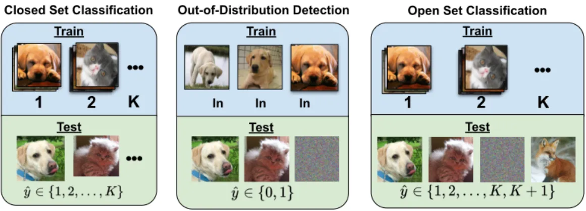
Open set classification (OSC) is the ability for a classifier to reject a novel input from classes unseen during training rather than assigning it an incorrect label [95]. This capability is particularly important for the development of 1) safety-critical software systems (e.g., medical applications, self-driving cars) and 2) lifelong learning agents that must automatically identify novel classes to be learned by the classifier [39, 40, 55, 82]. 1 2 K ? ? K In In Out-of-Distribution Detection In Train Test

Open Set Classification Train

1 2

Test Train

Closed Set Classification

Test

K

Figure 1.1: Open set classification is an extension of normal closed set classification where the model has the ability to reject a novel input from classes unseen during training rather than assigning it to an incorrect label.

The major challenge if OSC is one-class classification in the presence of ‘unknown unknowns’ since the set of possible inputs outside of the training set is unbounded. Within recent machine learning literature, the OSC problem is highly related to a number of different applications including selective classification [24], classification with a reject option [5, 49], and out-of-distribution (OOD) detection [20, 46, 67, 69]. For our work, the goal of an open set classifier is to correctly classify inputs that belong to the same distribution as the training set and to reject inputs that are outside of this distribution. This is a narrower definition than the broad application

(16)

CHAPTER 1. INTRODUCTION AND MOTIVATION 3 of OOD detection which is only concerned with finding a function to determine whether an input belongs to the training distribution and not concerned with the correct classification of samples which are in-distribution.

1.2

Continual learning for deep neural networks

While deep learning models are currently state-of-the-art for many computer vision tasks, there are times when they are ill-suited to specific applications. At this time one of those applications is updating in real-time a model to take into account new data or classes. Conventional deep learning models are trained slowly via stochastic gradient descent (SGD) by making multiple passes through a fixed training dataset. Once trained in this manner the model cannot be updated with new data without suffering catastrophic forgetting of the previously learned data representations [29]. This inability to build robust data representations from a multiple, dynamic (non-iid) data distribution is the goal of continual learning.

Continual learning strategies endeavor to overcome catastrophic forgetting through either architectural or unique training paradigms. All of these approaches are de-signed to bring down the computational cost involved in performing full rehearsal on previously learned data when a model needs to be updated with new knowledge [42]. They attempt to achieve nearly the same accuracy as offline learning without the overhead needed to store the entire training dataset and rehearse on it when new knowledge is acquired.

1.3

Objectives

This dissertation explores the design decisions in creating deep learning models for computer vision applications capable of open set classification and dealing with in-puts from unknown sources. It explores the tradeoffs in employing these techniques,

(17)

CHAPTER 1. INTRODUCTION AND MOTIVATION 4

Open Set Classification Train

1

2

Test

K

Open World Learning Train

Test

Agent Observing Data Time 1 1 ? 2 2

Figure 1.2: Open world learning involves learning to classify from dynamic data streams that are presented in a non-iid manner and may contain both labelled and unlabelled examples from open set classes.

how they may be applied to large-scale computer vision problems, and how models with this open set capability lead naturally to models which can continually learn from dynamic data distributions instead of being developed in distinct but archaic training and testing phases. The main objectives of our work include:

1. Critically evaluate the current state of outlier and novelty detection in deep neural networks

(a) Highlight how traditional outlier detection techniques are insufficient for novelty detection in deep learning models

(b) Describe efforts to adapt novelty detection for deep learning models and focus on the best performing models

(c) Demonstrate how current deep outlier detection models are insufficient for performing open set classification on large-scale computer vision datasets

(18)

CHAPTER 1. INTRODUCTION AND MOTIVATION 5 2. Develop a new method for model regularization that improves the feature

space of deep learning models for performing open set classification

(a) Identify elements of current model regularization strategies for open set classification that can be improved

(b) Demonstrate a novel training approach for building an open set classifier that is effective on large scale, challenging open set classification problems 3. Demonstrate how principles of open set classification can be applied to

con-tinual learning models

(a) Establish evaluation protocols for evaluating a model’s open set classifi-cation abilities when trained in a continual learning setting

(b) Outline principles of training a classifier and learning an effective feature representation for models trained in a continual learning setting that lead to high performance in both closed set and open set classification accuracy

1.4

Dissertation Layout

This dissertation consists of seven chapters including this introduction (Chapter 1) and a summary (Chapter 7).

1.4.1 Chapter 2: Open Set Classification for Deep Learning Model

in Computer Vision

We outline the current methods for performing open set classification in deep learn-ing models. We define the problem which consists of findlearn-ing a model that both classifies inputs to a known set of classes while also considering a separate func-tion for rejecting the input as belonging to an unknown class not specified during

(19)

CHAPTER 1. INTRODUCTION AND MOTIVATION 6 training. Currently the most successful rejection functions can be seen as a form of out-of-distribution detection where the acceptance score is determined based on some form of model confidence. We then outline other strategies for training a model that is more capable of open set classification as compared to standard cross-entropy training for supervised classification. Positive and negative aspects of each inference method and model regularization strategy are discussed.

1.4.2 Chapter 3: Survey of Large Scale Open Set Classification

Methods

In reviewing current open set classification methods, one shortfall in the current lit-erature is the lack of a comparison on large-scale problems where the in-distribution set contains hundreds to thousands of categories. Most methods to this point have only been tested on small datasets (e.g. CIFAR-10) which only consists of at most a hundred categories. We test the limits of many of the current state-of-the-art inference against a variety of challenging open set classification problems to find trends in performance and gaps which should be addressed in future work. Ad-ditionally no known work at this point has combined the current state-of-the-art inference methods for performing out-of-distribution detection with novel regular-ization methods we test different combinations of these two approaches to determine the optimal strategy for training a model capable of open set classification on large-scale datasets.

1.4.3 Chapter 4: Improved Feature Representations for Open Set

Classification in Deep Learning Models

Using lessons learned from evaluating current model regularization strategies for open set classification in large-scale image classification problems, we devise a new strategy for improving the current state-of-the-art methods. The best current

(20)

strat-CHAPTER 1. INTRODUCTION AND MOTIVATION 7 egy for training an open set classifier involves training with a background class as a proxy for potential unknown open set classes and using an auxiliary loss to separate known classes from the background. While this strategy has been demonstrated on many small toy datasets, extending its application to large-scale problems is problematic and less effective. Instead we propose a novel training scheme using the Mixup data augmentation scheme and a new loss we call, Tempered Mixup, to train the model to separate in-distribution inputs from potential open set classes. It relieves the user from having to create a background class from training and is more effective on most large-scale open set problems evaluated.

1.4.4 Chapter 5: Baselines for Open Set Classification in Continual

Learning Models

We detail the current methods and evaluation protocols used for continual learn-ing. We outline how continual learning can be evaluated on a spectrum of different training protocols and how streaming/online learning, or learning from one sample at a time is the most representative and difficult paradigm. We then characterize streaming learning into different sub-tasks based on the underlying ordering of the dataset and outline which datasets are available for each subtask. Finally after high-lighting the short coming of the available streaming learning datasets we introduce a new dataset, Stream-51, which is larger and more complex than other streaming datasets currently available. We also establish for the first time performance metrics on both closed set classification and open set classification for a handful of common streaming learning baselines.

(21)

CHAPTER 1. INTRODUCTION AND MOTIVATION 8

1.4.5 Chapter 6: Improving Open Set Classification in Streaming

Models

We analyze the principles behind performing open set classification in continual learning models and the properties that a successful deep learning model must pos-sess to succeed in this paradigm. We evaluate some of common strategies for per-forming streaming learning and evaluate what form of pre-training leads to the most successful streaming learner both in terms of closed set and open set classification. Finally we highlight some of the current gaps in improving streaming open set clas-sification and where further progress is likely to be made.

1.5

Related Publications

Portions of this dissertations have been published in the following outlets:

• Roady, Ryne, Tyler L. Hayes, Ronald Kemker, Ayesha Gonzales, and Christo-pher Kanan. ”Are Out-of-Distribution Detection Methods Effective on Large-Scale Datasets?.” PLOS One. 2020: e0235750.

• Roady, Ryne, Tyler L. Hayes, Hitesh Vaidya, and Christopher Kanan. ”Stream-51: Streaming Classification and Novelty Detection From Videos.” In Proceed-ings of the IEEE/CVF Conference on Computer Vision and Pattern Recogni-tion Workshops, pp. 228-229. 2020.

• Roady, Ryne, Tyler L. Hayes, and Christopher Kanan. ”Improved Robust-ness to Open Set Inputs via Tempered Mixup.” In Proceedings of the European Conference on Computer Vision Workshops. 2020.

(22)

Chapter 2

Background on Open Set

Classification for Computer

Vision

2.1

Introduction

To organize our overview of OSC methods in deep learning models, we separate the strategies for OSC into two general approaches. The first is specialized inference mechanisms for determining if the input to a pre-trained CNN should be rejected. The second is to alter the CNN during learning so that it acquires more robust representations of known classes that reduce the probability of a sample from an unknown class being confused. This often takes the form of collapsing class condi-tional features in the deep feature space of CNNs.

(23)

CHAPTER 2. BACKGROUND 10

2.2

Problem Definition

While OSC is related to uncertainty estimation [45] and model calibration [38], its function is to reject inappropriate inputs to the CNN. We formulate the problem as a variant of traditional multi-class classification where an input belongs to either one of theKcategories from the training data distribution or to an outlier/rejection category, which is denoted as the K+ 1 category. Given a training set Dtrain =

{(X1, y1),(X2, y2), . . . ,(Xn, yn)}, where Xi is the i-th training input tensor and yi ∈ Ctrain = {1,2, . . . , K} is its corresponding class label, the goal is to learn a

classifierF(X) = (f1, ..., fk), that correctly identifies the label of a known class and

separates known from unknown examples: ˆ y=    argmax_kF(X) ifS(X)≥δ K+ 1 ifS(X)< δ (2.1) where S(X) is an acceptance score function that determines whether the input belongs to the training data distribution andδ is a threshold.

For testing, the evaluation set contains samples from both the set of classes seen

during training and additional unseen classes, i.e.,Dtest={(X1, y1),(X2, y2), . . . ,(Xn, yn)},

where yi ∈(CtrainSCunk) and Cunk contains classes that are not observed during

training.

2.3

Current Approaches and Limitations

We have organized methods for OSC into two complementary families: 1) inference methods that create an explicit acceptance score function for separating novel inputs, and 2) regularization methods that alter the feature representations during training to better separate in-distribution and novel samples.

(24)

CHAPTER 2. BACKGROUND 11

2.4

Inference Methods: Outlier Detection in Pre-trained

Models

Inference methods use a pre-trained neural network to perform OOD detection, but modify how the network outputs are used. Using pre-trained networks is advanta-geous since no modifications to training need to be made to handle outlier samples, and the low-level features of pre-trained networks have been shown to generalize across different image datasets [115].

2.4.1 Output Layer Thresholding

The simplest approach to OOD detection is thresholding the output of a model, typ-ically after normalizing by a softmax activation function. For multi-class classifiers, the softmax layer assumes mutually exclusive categories, and in an ideal scenario would produce a uniform posterior prediction for a novel sample. Unfortunately, this ideal scenario does not occur in practice and serves as a poor estimate for un-certainty [31, 78]. Still, the largest output of the softmax layer follows a different distribution for OOD examples, i.e., in-distribution samples generally have a much larger top output than OOD samples, and can be used to reject them [46]. We refer to this output thresholding method as τ-Softmax, which computes the acceptance score as: S(F(X)) = max k exp (fk(X)) PK j=1exp (fj(X)) (2.2) wherefk(X) is the output logit for class k.

The Out-of-Distribution Image Detection in Neural Networks (ODIN) model [69] extends the thresholding approach by adjusting the softmax output through tem-perature scaling on the activation function given by:

σS(F(X);T)k=

exp (fk(X)/T) PK

j=1exp (fj(X)/T)

(25)

CHAPTER 2. BACKGROUND 12 where T is the temperature parameter used to soften the posterior distribution. ODIN also applies small input perturbations to the test samples based on the gradi-ent of this temperature adjusted softmax output. In this application, the sign of the gradient is used to enhance the probability of inputs that are in-distribution while minimally adjusting the output of OOD samples, i.e.,

˜

X=X−·sign (−∇_XlogσS(F(X);T)yˆ), (2.4)

where ˆy = maxkF(X) is the network prediction andis the magnitude of the

per-turbation. This perturbation method is motivated by [35], which used the gradient to generate adversarial examples that would enhance the posterior prediction of a desired class regardless of the input. These two adjustments further separate in-distribution and OOD samples, allowing for more accurate bounded classification without any changes to a network’s architecture or training paradigm [69].

Additionally, per-class thresholds can be set for sample rejection typically after using a sigmoid activation function on the output logit. The sigmoid activation helps to avoid the normalization properties of the softmax activation and create more discriminative per-class thresholds. This method is employed in the Deep Open Classification (DOC) model [98], which alters a typical multi-class CNN ar-chitecture by replacing the softmax activation of the final layer with a one-vs-rest layer containing K sigmoid functions for the K classes seen during training. A threshold, ki, is then established for each class by treating each example where y = ki as a positive example and all samples where y 6= ki as negative examples.

During inference, if all outputs from the sigmoid activations are less than the re-spective per-class thresholds, then the sample is rejected. For our evaluations, we separate this per-class thresholding strategy from the one-vs-rest model training strategy to isolate the benefits of each method.

(26)

CHAPTER 2. BACKGROUND 13

2.4.2 Distance Metrics

Outlier detection can also be done using distance-based metrics. Following the formulation of Knorr and Ng [59], a number of distance-based methods [2, 3, 6, 86] have been developed based on global and local density estimation by computing the distance between a sample and the underlying data distribution.

Euclidean distance metrics have been widely used [97, 104], but they often fail in high-dimensional feature spaces containing many classes. To mitigate this issue, [75] showed that the feature space of a neural network trained with cross-entropy loss approximates a Gaussian discriminant analysis classifier with a tied covariance matrix between classes. Under this assumption, a Mahalanobis distance metric can be used for generating a class-conditional outlier score from the deep features in a CNN, i.e.,

S(X) = min

k [G(X)−µk] T

Σ−1[G(X)−µk], (2.5)

where G(X) is an embedding of the input image from the CNN, µk is the mean

for class k and Σ is the average class conditional covariance in feature space. This approach is employed directly on CNNs by the Mahalanobis method [67], which computes a class-conditional Mahalanobis metric across multiple CNN layers and learns a linear classifier to combine these into a single acceptance score based on cross-fold validation. Similar to Eq. 2.4, Mahalanobis uses input perturbations as a pre-processing step, but computes the gradient with respect to the Mahalanobis distance rather than the softmax output. This increases the separation between in-distribution and OOD samples based on the assumption that in-in-distribution samples will be located on the regions of maximum gradient with respect to the class centers, whereas OOD samples will be more uniformly spread out in feature space. Because the OOD score is computed across multiple CNN layers, an additional linear classifier must be trained to combine the scores and make an overall OOD prediction. Unlike other methods, this process requires a validation set of both in-distribution and OOD

(27)

CHAPTER 2. BACKGROUND 14 samples. If the OOD validation set does not reflect the type of OOD examples seen during deployment, this approach may break down when deployed.

2.4.3 Extreme Value Theory

OOD detection methods based on extreme value theory (EVT) recognize novel in-puts by characterizing the probability of occurrences that are more extreme than any previously observed. This is typically implemented by characterizing the tail of class-conditional distributions in feature space. It has been directly adapted to CNN classifiers by modeling the distance to the nearest class mean in deep feature space as an extreme value distribution [93, 94] and calculating an acceptance score function as the posterior probability based on this EVT distribution. OpenMax [8] specifically applies EVT to construct a sample weighting function to re-adjust the output activations of a CNN based on a per-class Weibull probability distribution. The output is rebalanced between the closed set classes and a rejection class, and samples are rejected if the rejection class has a maximum activation or if the maxi-mum activation falls below a threshold set from cross-fold validation.

2.5

Model Regulariztion: Seperating Outliers in Deep

Feature Space

In contrast to methods that solely use the acceptance score function, we can address the problem of outlier detection in deep networks through model regularization to alter the architecture of the network or how the network is trained. These methods learn representations that enable better OOD detection performance.

(28)

CHAPTER 2. BACKGROUND 15

2.5.1 One-vs-All Training

The most common method for training a CNN classifier with K disjoint categories is using cross-entropy loss calculated from a softmax activation function. Although the softmax function is good for training a classifier over a closed set of classes, it is problematic for outlier detection because the output probabilities are normalized, resulting in high-probability estimates for inputs that are either absurd or intention-ally produced to fool a network [35, 78]. One-vs-rest classification models eliminate the softmax layer of a traditional closed-set classifier and replace it with a logistic sigmoid function for each class. While these per-class sigmoid activations no longer have a probabilistic interpretation in a multi-class problem, they reduce the risk of incorrectly classifying an OOD sample by treating each class as a closed-set classi-fication task, which can be individually thresholded to identify outliers. The DOC model is one version of a one-vs-rest classifier that replaces the traditional softmax layer with a one-vs-rest layer of individual logistic sigmoid units [98].

2.5.2 Background Class Regularization

Another method for improving OOD detection performance via feature space regu-larization is using a background class to separate novel classes from known training samples. This technique is most commonly applied in object detection algorithms where the use of separate region proposal and image classification algorithms re-sult in a classifier that must handle ambiguous object proposals [89]. Often these classifiers represent the background class as a separate output node which is trained using datasets that have an explicit ‘clutter’ class such as MS COCO [71] or Caltech-256 [37]. Alternatively, newer approaches have used background samples to train a classifier to predict a uniform distribution when presented with anything other than an in-distribution training sample [47]. This is done through various regular-ization schemes including confidence loss [66] and the objectosphere loss [22] which

(29)

CHAPTER 2. BACKGROUND 16 have shown better performance than using a separate output node. Nevertheless, for modern image classification datasets which may have 1,000+ classes, finding explicit background samples that are exclusive of the training classes has become exceedingly difficult.

Generative Models

Using CNNs for generative modeling has been an active area of research with the advent of generative adversarial networks [34] and variational auto-encoders [57]. Generative models have extended earlier density estimation approaches for outlier detection by more accurately approximating the input distribution. A well-trained model can be used to directly predict if test samples are from the same input distri-bution [76] or estimate this by measuring reconstruction error [81]. Paradoxically, generative models have also been used to create OOD inputs from the training set in order to condition a classifier to produce low confidence estimates similar to how an explicit background class is used for model regularization [66, 77, 116].

2.6

Qualitative Assessments

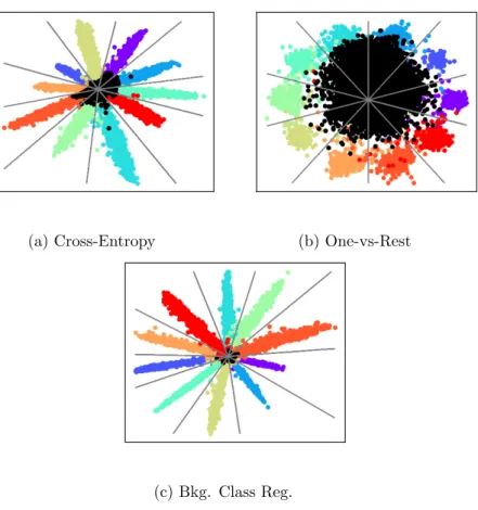
To visually illustrate the differences between various methods, we trained a simple model for outlier detection using the MNIST dataset. We used a shallow CNN with a bottle-necked feature layer, i.e., the LeNet++ architecture [65], to allow visualization of the resulting decision boundaries. Fig. 2.1 shows the 2-D decision boundaries with blue representing in-distribution classification at a 95% true positive rate threshold and red representing the resulting rejection region. Additionally, we mapped samples from an unknown class represented by the Fashion-MNIST [113] dataset in Fig. 2.2 to understand how the decision boundaries relate to the deep CNN features of known and unknown classes.

(30)

CHAPTER 2. BACKGROUND 17 T est Data and Class Boundaries Confidence Thresholding T emp Scaling Ext V al Theory (Op enMax) One-Class SVM Mahalanobis Dist Thresholding Cross-En trop y One-vs-Rest (Binary Cross-En trop y) Bac kground Class Regularization Figure 2.1: 2-D visualization of the decision b oundaries created from the differen t OOD inference metho ds studied using the LeNet+ arc hitecture and MNIST [65] as the tr aining set. Blue is the acceptance region for in-distribution samples calibrated at a 95% T rue P ositiv e Rate (TPR) for training data. Red is the rejection region (outlier).

(31)

CHAPTER 2. BACKGROUND 18

(a) Cross-Entropy (b) One-vs-Rest

(c) Bkg. Class Reg.

Figure 2.2: 2-D visualization of the effect of the different feature space regulariza-tion strategies on separating in-distriburegulariza-tion and outlier inputs The in-distriburegulariza-tion training set is MNIST while the OOD set is Fashion-MNSIT [113]. For back-ground class regularization, the EMNIST-Letters dataset [16] is used as a source for background samples

(32)

CHAPTER 2. BACKGROUND 19 These results illustrate that for a given feature space, inference strategies can be divided between those that have unbounded acceptance regions (e.g.,τ-Softmax) with those that are bounded (e.g., OpenMax). Much has been made of this dis-tinction [95] and it is seen as a strength of the inference methods with bounded regions. However, as Fig. 2.2 represents, unknown inputs are rarely mapped into these unbounded regions, but rather are centered around the origin in the deep fea-ture space of a CNN. This implies that properly mapping the acceptance/rejection region around the origin is critical performance. Of the bounded acceptance region methods, OpenMax and Mahalanobis create the most compact decision boundaries. However, having compact boundaries may not be the best option when generaliza-tion to test inputs and unknown novel inputs is desired.

The goal of different feature space regularization strategies is to build robustness into the deep feature space by separating knowns from potential unknowns. While naively the One-vs-Rest training strategy appears to be a good solution by creating more compact class conditional distributions, the technique does not directly impact how features from unknown inputs will be mapped into the deep feature space. Instead we see that regularizing the model with a representation of the unknown class creates better separation between the known and unknown [22,66]. The difficulty in this approach, however, lies in large-scale datasets with many hundreds of classes.

Current OSC research has either focused on developing inference strategies for pre-trained models or a feature representation strategy for baseline inference meth-ods. To minimize open-space risk, an OOD inference method should create a com-pact decision boundary around the known classes in feature space. To facilitate this, an ideal CNN should train to have compact class-conditional distributions in feature space that are regularized against some representation of the unknown.

(33)

CHAPTER 2. BACKGROUND 20

2.7

Open Questions for OSC in Deep Learning Models

The vast majority of prior work for OSC in image classification has focused on small, low-resolution datasets, e.g., MNIST and CIFAR-100. Deployed systems like autonomous vehicles, where outlier detection would be critical, often operate on images that have far greater resolution and experience environments with far more categories. It is not clear from previous work if existing methods will scale. In the following sections of this thesis we will compare methods across open set classification paradigms on large-scale, high-resolution image datasets.

(34)

Chapter 3

Large-Scale Open Set

Classification

3.1

Introduction

In this chapter, we desire to understand open set classification performance as a function of multiple variables. First we want to understand how the requirement to detect data from unknown classes is affected by dataset scale both for the training set and the evaluation set which includes open set classes. The modern boom in deep learning approaches has been largely enabled by relatively new large scale datasets that include hundreds of classes and millions of overall training samples (images). We desire to understand ultimately how open set performance is affected as both the overall number of classes in the training set is increased and as the overall number of samples. Additionally we want to understand how the complexity of the open set classes in the evaluation set affects overall performance.

Next, the other enabling technology in state-of-the-art deep learning networks has been the development of deeper networks with hundreds of convolutional filters per layer. Previous work has shown that deeper and wider networks produce more

(35)

CHAPTER 3. LARGE-SCALE OPEN SET CLASSIFICATION 22 accurate results but often lead to calibrated predictions [38]. We desire to un-derstand if there was a correlation between model capacity in a CNN, i.e., the depth and width of convolutional layers, and the resulting OSC performance.

Finally, we look to understand how different commonly used regularization schemes in training deep networks affects OSC performance. In general, model regu-larization strategies, including both auxiliary loss functions and data augmentation techniques, are introduced during training to prevent over-fitting to the training set and improve generalization to unseen samples from the closed set of classes in the evaluation set. It is logical to assume that improving generalization might also improve model calibration by preventing the model to be overly confident; however, it is not clear how this performance would translate to recognizing examples as novel that may be similar to the training classes but are ultimately from open set classes. We perform experiments to test the effect of common regularization schemes on OSC performance and hypothesize why some regularization types improve OSC performance more than others.

3.2

Assessment Details

To quantify OSC performance, we use two separate metrics for evaluation. First we use the area under the receiver operating characteristic curve (AUROC) metric to assess OSC performance of each approach as a binary detector for separating in-distribution and outlier samples. AUROC characterizes the performance across a full range of threshold values, regardless of the range of unique values for each inference method’s scoring function. AUROC has been a commonly used metric for measuring OOD detection capabilities in image classification datasets [46, 47, 66, 67, 69]. This metric is best suited for comparing the inference methods which use the same pre-trained model; however, when comparing regularization techniques where the underlying closed-set accuracy can differ between models, we want a more

(36)

CHAPTER 3. LARGE-SCALE OPEN SET CLASSIFICATION 23 discriminating measure.

Thus, we also adopt the area under the open set classification characteristic curve [22] (AUOSC), which is an adaptation on the traditional ROC curve mea-suring instead the correct classification rate versus false positive rate. This correct classification rate is the difference between the model accuracy and the false nega-tive rate. Intuinega-tively, this metric takes into account whether true posinega-tive samples are actually classified as the correct class and thus rewards methods which reject incorrectly classified positive samples before rejecting samples that are correctly classified. We extend the open set classification characteristic curve from [22] to calculate the area under the curve which provides an easy assessment of perfor-mance across different experimental paradigms and datasets.

To estimate the ability of OSC methods to scale, we trained models on the Im-ageNet large-scale image classification dataset (ImIm-ageNet). The ImIm-ageNet dataset was part of the ImageNet large-scale Visual Recognition Challenge [92] between 2012 and 2017 and evaluated an algorithm’s ability to classify inputs into one of 1,000 possible categories. The dataset consists of 1.28 million training images (732-1300 per class) and 50,000 labeled validation images (50 per class), which we use for evaluation. We train an 18-layer ResNet model [44] for image classification on 500 randomly chosen classes, reserving the remaining 500 for intra-dataset OSC experiments.

To train the models, we use stochastic gradient descent with a mini-batch size of 256, momentum weighting of 0.9, and weight decay penalty factor of 0.0001. All models are trained for 90 epochs, starting with a learning rate of 0.1 that is decayed by a factor of 10 every 30 epochs. Training parameters were held constant for all feature space regularization strategies unless otherwise noted. The baseline cross-entropy trained model for the 500 class partition achieves 78.04% top-1 (94.10% top-5) accuracy.

(37)

CHAPTER 3. LARGE-SCALE OPEN SET CLASSIFICATION 24

3.2.1 Inference Method Comparison

To begin our assessment, we compare six of the inference methods described in Sec. 2.4 on large-scale image classification datasets using a pre-trained deep CNN model trained with cross entropy loss. We summarize their acceptance score func-tions and inference complexity in Table 3.1. The specific implementation details for the inference methods evaluated are as follows:

1. τ-Softmax– This simple baseline approach finds a global threshold from the final output of the model after the associated activation function is applied. The method yields good results on common small-scale datasets [46] and can be easily extended to datasets with many classes.

2. DOC – Per-class thresholding has been shown to successfully reject outlier inputs during testing on common, small-scale datasets [99]. Adapting this method to larger datasets is more computationally expensive thanτ-Softmax because a per-class threshold must be established.

3. ODIN – This approach can outperform τ-Softmax when using well-trained CNNs; however, the technique adds computational complexity during infer-ence to calculate input perturbations [69]. ODIN also adds additional hyper-parameters for the magnitude of input perturbation and a temperature scaling factor which must be determined through cross-validation.

4. OpenMax – OpenMax is one of the only methods previously tested on Im-ageNet [8]. It models a per-class EVT distribution and has multiple hyper-parameters that must be tuned through cross-validation making it relatively cumbersome to use for large-scale datasets during training. Once these pa-rameters have been found, however, it presents a robust inference method for estimating whether a sample belongs to one of the known classes or to an explicitly modeled outlier class. In the original implementation the decision

(38)

CHAPTER 3. LARGE-SCALE OPEN SET CLASSIFICATION 25 rule for rejection involves a two step process where a sample is rejected as novel if either the outlier class is largest or the maximum class confidence of in-distribution classes is below a user-defined threshold. Because we evaluate methods across a range of thresholds, we have simplified this decision rule by setting the model confidence to zero if the outlier class is largest, otherwise the largest non-outlier confidence class is returned as the acceptance score value. 5. One-Class SVM – One-class SVMs have been employed as a simple

unsu-pervised alternative to density estimation for detecting anomalies. They have been tested across a wide variety of datasets, but not on the large-scale image datasets and CNN architectures used in this analysis. We use a radial basis function kernel to allow a non-linear decision boundary in deep feature space and tune hyperparameters via cross-validation.

6. Mahalanobis – In [67], the Mahalanobis metric was computed at multiple layers within a network and then combined via a linear classifier that was calibrated using a small validation set made up of in-distribution and outlier samples. To avoid biasing the model by training with open set data, we only compute the Mahalanobis metric in the final feature space. Adapting this metric to a large-scale dataset is straightforward, however, there is additional computational and memory overhead to estimate and store class conditional means and a global covariance matrix in feature space.

Hyperparameters for each inference method are tuned using outlier samples drawn from uniform noise to avoid unfairly biasing results to the datasets used for evaluation. Performance of each of the inference methods listed is shown in Fig. 3.1.

Because the OSC performance increase from ODIN comes at a computational and memory cost, we also want to understand which elements of the inference

(39)

CHAPTER 3. LARGE-SCALE OPEN SET CLASSIFICATION 26 Table 3.1: The studied inference methods for OOD detection. Inference complexity refers to the number of passes through a deep CNN (forward and backward) during inference. Classification Method Acceptance Score Function Inference Complexity τ-Softmax [46] Simple Threshold 1 DOC [98] Per-Class Threshold 1 ODIN [69] Temp Adjusted Threshold 3 OpenMax [8] Per-Class EVT Rescaling 1 One-Class SVM [96] SVM Score 1 Mahalanobis [67] Generative-Distance Metric 3

method contribute most to the overall improvement in order to find the most effi-cient application of computational resources for OSC. To do this we performed an ablation of the method by looking at the OSC performance gained from temperature scaling and input perturbation independently as shown in Fig. 3.2. For temperature scaling, we performed two variations: one where the temperature is chosen based on the procedure to minimize overall model calibration error as outlined in [38] and another where we grid search on a leave-out validation set for the best temperature for OSC performance independent of the impact on overall model calibration or closed set classification performance.

3.2.2 OSC Similarity Comparison

To evaluate the large-scale open set classification capabilities across a variety of OOD datasets, we created three separate outlier detection problems that vary in difficulty:

(40)

CHAPTER 3. LARGE-SCALE OPEN SET CLASSIFICATION 27

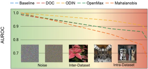
Figure 3.1: Specialized Inference Methods for Large-Scale OSC. Left) The ROC curve for various inference methods designed to determine whether samples are from known classes seen during training or from an unknown class. A ResNet-18 model is trained on a split made up of 500 randomly chosen categories from ImageNet. Evaluation is performed on the full ImageNet validation set with categories unseen during training being labeled as unknown (negative category). Right) The relative memory and computational cost of these specialized inference methods is shown relative to baseline confidence thresholding.

(41)

CHAPTER 3. LARGE-SCALE OPEN SET CLASSIFICATION 28

Figure 3.2: Effects of Input Perturbation and Temperature Scaling. An ablation experiment for detecting intra-dataset open set classes on a ResNet-18 model trained on 500 classes of ImageNet. As shown an optimal temperature scaling factor provides much of the overall performance benefit from the ODIN method with virtually no increase in computational complexity.

1. Noise: As the easiest OSC task, we evaluate both uniform and Gaussian noise inputs, which has been widely studied as a baseline [46, 61, 66, 69]. For the Gaussian images, we generate synthetic images from a zero mean, unit variance Gaussian distribution to match the data normalization scheme used for training our models.

2. Inter-Dataset: As a problem of intermediate difficulty, we study each method’s ability to detect outlier samples drawn from a separate medium to high resolu-tion image classificaresolu-tion dataset. We include samples drawn from the Oxford Flowers dataset [79] and select categories of the Places dataset [120]. Specif-ically we removed overlapping categories from the Places dataset with our ImageNet training set determined using the hypernym/hyponym relationship from the Wordnet lexicon [27]. Additionally, for the Places dataset we sampled only from the outdoor categories leaving the indoor categories for regulariza-tion experiments as described below.

(42)

CHAPTER 3. LARGE-SCALE OPEN SET CLASSIFICATION 29 3. Intra-Dataset: As the hardest outlier detection task, we used the remaining

500 categories from ImageNet that were not used for training.

In summary, the training set and models are kept fixed across the three paradigms, but the test sets vary across them. We construct the open set evaluation samples for each problem by randomly choosing 10,000 in-distribution samples evenly among the in-distribution classes and 10,000 outlier samples evenly among the open set classes within each respective dataset’s validation set. This evaluation process was repeated 5 times and the resulting metrics were averaged.

To plot OSC performance across the varying OOD datasets against a meaningful metric, we use the maximum mean discrepancy (MMD) metric with a Gaussian kernel [101], i.e., ˆ M M D2(P, Q) = 1 N X i6=j G(pi, pj) + 1 N X i6=j G(qi, qj)− 2 N X i6=j G(pi, qj)

where P and Q are the in-distribution and OOD sample spaces respectively and

G(·,·) is a Gaussian kernel whose scaling parameter is set to the median Euclidean distance of the aggregate set (P∪Q). MMD is commonly used for quantifying the distance between datasets drawn from different distributions. Using this metric, we plot the OSC performance as a function of the MMD similarity in Fig. 3.3.

3.2.3 Regularization Comparison

Finally to assess the benefit of feature space regularization, we tested across three different training paradigms, including standard cross entropy training. The feature space regularization strategies for improving outlier detection were implemented as follows:

1. Cross-Entropy– As a baseline, we train each network with standard cross-entropy loss to represent a common feature space for CNN-based models.

(43)

CHAPTER 3. LARGE-SCALE OPEN SET CLASSIFICATION 30

Figure 3.3: In-distribution / OOD Similarity Comparison. AUROC for OSC as a function of the MMD metric (log-scale, axis-reversed) measured from ResNet-18 embeddings for each dataset tested. For all methods tested, there is a large decrease in open set accuracy as the difference in feature representations of in-distribution and open set datasets decreases

2. One-vs-Rest– The one-vs-rest training strategy was implemented by substi-tuting a sigmoid activation layer for the typical softmax activation and using a binary cross-entropy loss function. In this paradigm, every image is a negative example for every category it is not assigned to. This creates a much larger number of negative training examples for each class than positive examples. For this reason, we re-weight the negative-class training loss to be proportional to the positive-class loss to ensure comparable closed-set validation accuracy. 3. Background Class Regularization – The Entropic Open Set method [22] is a regularization scheme which uses a background class and a unique loss function during training to optimize the feature space of a neural network for

(44)

CHAPTER 3. LARGE-SCALE OPEN SET CLASSIFICATION 31 separating known classes from potential unknowns. Similar to the confidence loss term in [66], the Entropic Open Set loss forces samples from the back-ground class to the null vector in feature space by calculating the cross-entropy of a uniform distribution for these samples. An additional regularization term is used to measure the hinge loss of the magnitude between samples in the background class and the training samples in feature space. For the back-ground class, we use samples drawn from classes in the Places dataset that do not overlap with ImageNet classes and are distinct from the classes in the Places OSC experiments.

For background class regularization of an ImageNet trained model, we use the Places dataset, which contains high-resolution images of scenes which are grouped into categories based on their human-related function [120]. We removed 103 cat-egories from Places that overlapped with ImageNet, which were determined using the hypernym/hyponym relationship from the Wordnet lexicon [27]. The remain-ing classes were then split into outdoor and indoor sub-groups. The indoor classes are used for training models that require background class regularization, while im-ages from the outdoor classes are used for our inter-dataset OSC experiments of intermediate difficulty. Results from these experiments are shown in Table 3.2.

In Fig. 3.4 we also show the resulting ROC curves for the ImageNet Intra-Dataset problem across the three feature spaces tested, which demonstrate that there is little to no benefit from background class regularization versus standard cross-entropy training in the open set classification task.

3.2.4 Model Depth and Width

Current state-of-the-art networks on large-scale image datasets often have hundreds of layers and hundreds of convolutional filters per layer. Previous work has shown that deeper and wider networks produce more accurate results, but often lead to

(45)

CHAPTER 3. LARGE-SCALE OPEN SET CLASSIFICATION 32 Table 3.2: Area Under the Open Set Classification curve (AUOSC) for outlier detec-tion and open set classificadetec-tion performance in ImageNet trained models averaged over 5 runs. Top performer for each in-distribution / OOD combination is in blue along with statistically insignificant differences from the top performer as deter-mined by DeLong’s test [19] (α = 0.01 with a correction for multiple comparisons within each column).

Features Space Inference Method Gaussian Places-Out ImageNet-Open

CrossEntropy τ-Softmax 0.786 0.713 0.688 DOC 0.786 0.713 0.688 ODIN 0.787 0.744 0.714 OpenMax 0.786 0.712 0.687 One-Class SVM 0.744 0.632 0.632 Mahalanobis 0.751 0.523 0.502 One-vs-Rest τ-Softmax 0.649 0.539 0.539 DOC 0.633 0.483 0.483 ODIN 0.650 0.560 0.560 OpenMax 0.649 0.500 0.500 One-Class SVM 0.637 0.499 0.499 Mahalanobis 0.623 0.439 0.439

Background Class Regularization

τ-Softmax 0.751 0.746 0.717 DOC 0.751 0.746 0.720 ODIN 0.784 0.765 0.739 OpenMax 0.734 0.672 0.737 One-Class SVM 0.743 0.719 0.719 Mahalanobis 0.750 0.545 0.493 uncalibrated predictions [38].

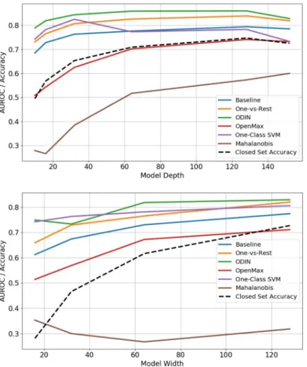
As an additional experiment, we desire to understand if there is a correlation between model capacity in a CNN, i.e., the depth and width of convolutional layers, and the resulting OSC performance. Our results indicate that in general novelty detection performance is related to overall model accuracy and varies as the feature

(46)

CHAPTER 3. LARGE-SCALE OPEN SET CLASSIFICATION 33

(a) Cross-Entropy (b) One-vs-Rest

(c) Background Class Reg.

Figure 3.4: ROC curves for the ImageNet / Intra-Dataset (Open Set) test.

space representation changes. To answer this question, we follow the protocol of [38] and train a series of ResNet models with either a fixed convolutional filter width (64) and varying depths (10-152 layers) or fixed depth (18 layers) and varying number of filter channels per layer (16-128). The results from these experiments are shown in Fig. 3.5. Since performance on detecting open set samples largely tracks overall model accuracy it is not overly surprising that as the depth and width grow and model accuracy increases, then outlier detection performance also increases. Unlike the previously reported negative effect of model capacity on confidence calibration, there is no indication that increasing model depth or width negatively impacts OSC performance.

(47)

CHAPTER 3. LARGE-SCALE OPEN SET CLASSIFICATION 34

Figure 3.5: Examination of OOD detection performance as a function of model capacity. A ResNet architecture was varied in either depth or width and trained on the ImageNet-500 split and then tested for detecting image classes unseen during training via either the Places dataset (Inter-dataset) or the remaining ImageNet categories (Intra-dataset). Overall improvements in performance as reflected in the AUROC of the model track improvements in model accuracy as model capacity increases.

(48)

CHAPTER 3. LARGE-SCALE OPEN SET CLASSIFICATION 35

3.2.5 Discussion

For inference methods, we see that ODIN performs best on detecting open set classes from the ImageNet dataset for a pre-trained model across all three feature space reg-ularization methods and across all outlier datasets evaluated. These results show the power of input perturbation and temperature scaling by showing improved per-formance over baseline methods and even more advanced methods on ImageNet, regardless of the feature space and difficulty of the OSC problem. However, this improvement comes at nearly a third reduction in image throughput and more than three times the memory cost during inference (see Fig. 3.1). Results among the re-maining inference methods are mixed, with the baseline global thresholding method (τ-Softmax) performing equal to or better than all other methods for the most diffi-cult, open set, outlier detection problem. Finally, while in general OSC performance decreases as the similarity between the OOD and in-distribution data increases, the relative performance increase of the ODIN method above the other methods tested is consistent across the different OOD datasets tested.

A large portion of the performance gain from ODIN can be achieved through temperature scaling alone as shown in Fig. 3.2, which comes at virtually no increase in computational complexity or memory cost during inference as compared to the input perturbation method. This appears contradictory to recent improvements in OSC [20, 67] which have solely focused on utilizing the input perturbation methods to improve performance. Additionally our experiments show that finding a temper-ature scaling factor to optimize OSC performance is a separate task than finding the optimal temperature for minimizing calibration error.

Additionally, looking closer at the benefit of the different feature space represen-tation methods tested, the results are mixed depending on the difficulty of the OSC problem. In general one-vs-rest training, results in reduced overall classification per-formance as seen in the lower AUOSC results which makes it a less desirable option

(49)

CHAPTER 3. LARGE-SCALE OPEN SET CLASSIFICATION 36 for actually performing open set classification. Further, the benefit of background class regularization is demonstrated most significantly when detecting outlier sam-ples that are similar to the background dataset used for training. The quantity of this improvement is reduced, however, as the OSC problem becomes more difficult. Nevertheless, background class regularization did not hurt either outlier detection or open set classification performance for any inference method except the Mahalanbois method.

Fundamentally, the increase in OSC difficulty as the similarity increases between OOD and in-distribution samples is due to the network confusing OOD inputs with known classes. This confusion stems from the feature space of the CNN classifier which learns to be most sensitive to variations in the training distribution that are semantically meaningful while ignoring variations that are not semantically mean-ingful among the known classes. Dealing with semantically meanmean-ingful variations in images from both known and unknown classes that are not included in the training set is ultimately the most significant problem in the OSC process.

Research in OSC has largely focused on either developing inference strategies for pre-trained models or a feature representation strategy for baseline inference meth-ods for detecting outlier samples. However, as our results show, a large performance increase can be gained by combining an advanced inference technique with a feature space regularization strategy. Nevertheless, the performance increase over baseline techniques appears to be much smaller as the dataset becomes more complex and the novelty detection problem becomes more difficult.

(50)

Chapter 4

Improved Feature

Representation for Open Set

Classification in Large-Scale

Models

4.1

Introduction

In this chapter we describe our process for improving representations for open set classification. The current inference strategies which are covered in the background form the basis for our new approach which builds a better feature space representa-tion for applying these open set classificarepresenta-tion methods to large scale datasets without the use of a background class in training. These OOD inference methods can be greatly improved by using a straight forward regularization scheme that makes com-parisons between classes and open-space more accurate with minimal impact to the generalization capability of the classifier. Our goal is to find a way that can improve the detection of novel classes without the reliance of a non-overlapping background

(51)

CHAPTER 4. IMPROVING OPEN SET CLASSIFICATION 38 class which is problematic to derive for datasets which contain a large amount of classes. Our process which we title Tempered Mixup is a data augmentation scheme paired with a unique auxiliary loss formulation.

Data augmentation is a very common practice in deep learning models to pre-vent over-fitting to training data and increase model robustness to various input corruptions. For basic training methods of deep learning models, random mirroring of the image along the horizontal axis and cropping and resizing to different scales are common practices used in state-of-the-art models [44]. Additionally, work has been performed to learn which from a series of potential image manipulations (e.g. translation, shearing, contrast/color adjustment, etc.) can be combined to most improve model performance. This technique which is known as Auto-Augment has been performed to improve both raw model accuracy [18] and model robustness to corrupted imagery [48].

Further, recent research has shown that more sophisticated augmentation such as random occlusions and random blurring of small sections of the image may improve accuracy on clean data and improve robustness to similar image corruptions [20]. Further the technique called CutMix, replaces a small section of the image with a portion of different image in the training set rather than just occluding it with the hope of finding a more well behaved model when dealing with samples that may not be accurately represented in the training data [117]. Finally, most relevant to our method is the data augmentation technique known as Mixup which also combines two separate images from the training set into a single example by forming a element-wise convex combination of the two input samples [118]. This technique has proven to be very successful by both improving model accuracy as originally proposed and in other applications by improving model calibration [105] and model robustness to certain types of image corruptions [15]. Interestingly thought one area where mixup augmentation has not shown to improve deep learning classification performance is

(52)

CHAPTER 4. IMPROVING OPEN SET CLASSIFICATION 39 in the area of open set classification and out-of-distribution detection. Specifically in [15], a 50% reduction in OOD detection performance on models when mixup is used versus baseline cross entropy loss training and confidence thresholding to identify OOD samples.

A simple method related to input augmentation which has also show promise for improving model robustness is label perturbation. In general this method works by penalizing over-confident predictions by perturbing the target during training thus resulting in an improved calibration of predictive uncertainty in the model. The simplest application of this strategy is label smoothing [103] which changes the ground-truth label to a smoothed distribution whose probability of non-targeted labels areα/Kwhereαis a user defined smoothing parameter andK is the number of classes. This process has been shown to offer a modest amount of robustness to unknown input corruptions [54] but results for improving OOD detection versus even simple outlier distributions has been mixed [15].

As an alternative to data augmentation policies, auxiliary losses have a long history in machine learning for encouraging certain model behaviors. L2 or L1

regularization has long been used to reduce model over-fitting to training data and improve generalization by directly penalizing large parameter values within a model which then produce smaller feature space activation. Recently, direct regularization of the feature space representation has been used to improve different aspects of model performance. Center Loss [109] penalizes the euclidean distance between a samples feature space representation and the associated class mean thus reducing the inter-class variance and creating more compact class-conditional distributions in deep feature space. It has been used extensively in many face identification deep learning models [72, 107, 111] where a single class must be recognized against a background of potential imposters [70].

(53)

multi-CHAPTER 4. IMPROVING OPEN SET CLASSIFICATION 40 class classification model to improve detection of outlier classes. The loss is a simple addition to standard cross entropy loss training

L_conf =    −logSk(F(X)) ifX∈Dtrain −1 K PK k=1logSk(F(X)) ifX∈Dbkg (4.1) where the first term of samples fromDtrainis standard training for in-distribution

training, but the second loss term over samples fromDbkg forces the model to push

samples from a representative background class toward a uniform posterior distri-bution. When a model is trained in this manner it has been shown that this also results in background samples being mapped to the null space of the deep feature space embedding prior to classification.

4.2

Background Class Selection for Confidence Loss

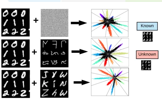
The difficulty in applying confidence loss to large-scale visual recognition problems such as the ImageNet dataset stems from the problem of background selection. Multiple approaches have been developed for producing open set images including using alternative datasets which are distinct from the training set [22, 85] and even using generative methods to produce images outside of the manifold defined by the training set [66,77]. Naturally, the performance of the open set classifier trained with open set images is tied to the “representativeness” of the background dataset and its similarity to the known training set. We first demonstrate this effect looking at the feature space learned for MNIST classification under various types of background datasets. As shown in Fig. 4.1, when the potential unknowns (in this case the Extended-MNIST letters dataset) are very similar to the known data the resulting robustness gained is very dependent on the properties of the background set.

The difficulty for even small-scale classification is that the effectiveness of certain background sets cannot be known a priori and seemingly representative background datasets can sometimes fail to produce better open set robustness. We demonstrate

(54)

CHAPTER 4. IMPROVING OPEN SET CLASSIFICATION 41

+

Known Unknown

Figure 4.1: LeNet++ Feature Space from Various Background datasets. The result-ing robustness to inputs from novel categories is shown after trainresult-ing with various background datasets. Because the unknown dataset is very similar to the set of training data little robustness is gained from background images that don’t explictly contain the open set classes. Additionally even when these classes are included there is still some class confusion that can occur as shown in the bottom feature space.

this phenomenon further using the CIFAR-10 dataset and a 32-layer ResNet model in Fig. 4.2. As shown, if a background class is not chosen carefully the resulting model will not perform well in detecting outlier examples across the full range of potential sources. In particular there is a clear relationship between the similarity of the background class to the in-distribution set and the resulting OOD performance. An appropriate background class should be as close to the in-distribution as possible (as illustrated in the Maximum Mean Discrepancy metric) while avoiding too close of a semantic overlap to the in-distribution classes. However, if a background class

(55)

<