1435
Application Of Hyperparameter Optimized Deep
Learning Neural Network For Classification Of Air
Quality Data
Anvesh Parashar, Abhilash SonkerAbstract: In recent year machine learning algorithms found several applications in different domains like image processing, natural language processing, pattern recognition and various data mining application, especially deep learning neural network have proved its capabilities in every major machine learning application. One such application is Ambient air quality prediction and classification. Due to deteriorating air quality special efforts are being made all over the world by different agencies to model and counter air pollution using machine learning algorithm for making state of the art prediction models. But choice of these model is solely based on trial and adapt method and an approach to optimize hyperparameter of the chosen model is needed. This paper focusses on some basic application of Deep Learning Neural Network to classify the air quality data and use of hyperparameter optimization using Talos for deployment of the model.
Index Terms: Air Quality Index (AQI), Data Mining Deep learning neural networks, Hyperparameter, Hyperparameter optimization, Machine Learning Algorithms, Talos.
—————————— ——————————
1.
INTRODUCTION
n recent year the machine learning emerged as a lucrative method to analysis and model huge amount of data with very high accuracy and precision. Machine Learning Algorithms consist of various state of the art Algorithms that are used to implement various analytical and prediction-based application on data that no other model can comprehend. One such successful application is Artificial neural network in machine learning. The motivation for this research comes from various negative effects associated with a sudden rise of air pollutants globally especially in urban areas. In this paper a deep learning neural network implemented using Keras [20] is used to classify the air quality data, though the traditional approach uses trial and error for hyperparameter optimization. That means a number of models are tested for optimal solution before deployment or pre-trained models are used. Here we have used a special library ―Talos‖ [21]to scan the permutation space of hyperparameters for finding the optimal hyperparameter for our model. Here the research is limited to classification using our model but this can be further extended for other deep learning neural networks for optimizing their hyperparameter.
1.1 AIR QUALITY INDEX (AQI)
Air quality is deteriorating globally especially in urban areas. Due to risk factors associated with rising air pollutants concentration and health risk inhaling polluted air, many agencies are established to monitor and counter such changes in ambient air. These agencies monitor air quality periodically and suggest counter measures to the government agencies earlier for swift action regarding the same. The monitoring station are sparsely located and coarsely record data in fixed intervals such as 1 hours, 8 hours, 24 hours etc. Though many pollutants are monitored in standard monitoring protocols but here we are using only four major pollutants
namely PM10, PM2.5, SO2, NO2. Daily pollutants concentration information is important for citizens especially those who can be affected by exposure to air pollution. Further it is important for a nation to improve its air quality and thus a simple and effective concept is needed by which a citizen or a government can assess the air quality .The concept of Air Quality Index is proposed to solve this problem.it is transformed weight values of individual air pollution related parameters into a single indicator that can be used to assess the air quality effectively. An AQI system is devised under Indian national Air Quality Standards (INAQS). Maximum operator is used to transform all sub-indices for each pollutant into a single index that is maximum of all indices is adopted as an overall AQI.
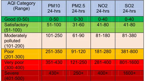
The current Index used in INAQS has six categories shown below in an elegant color scheme.
Good (0-50)
Satisfactory (51-100)
Moderately polluted (101-200)
Poor
(201-300)
Very poor (300-400)
Severe (>401)
Figure 1 color scale of AQI
The mathematical equation used for calculating AI for any pollutants is given by:
𝐴𝑄𝐼 =
[ ( )
] (𝐶 − 𝐵
) + 𝐼 (1)
Where
𝐶 =actual concentration of any pollutant,
𝐵
& 𝐵 =
𝑡𝑒 𝑖𝑔 𝑎𝑛𝑑 𝑙𝑜𝑤 𝑣𝑎𝑙𝑢𝑒𝑠 𝑐𝑜𝑟𝑟𝑒𝑠𝑝𝑜𝑛𝑑𝑖𝑛𝑔 𝑡𝑜 𝑡𝑒 𝑏𝑟𝑒𝑎𝑘 𝑝𝑜𝑖𝑛𝑡 𝐼 = 𝑡𝑒 𝑠𝑢𝑏 𝑖𝑛𝑑𝑒𝑥 𝑣𝑎𝑙𝑢𝑒 𝑐𝑜𝑟𝑟𝑒𝑠𝑝𝑜𝑛𝑑𝑖𝑛𝑔 to𝐵
𝐼 = 𝑡𝑒 𝑠𝑢𝑏 𝑖𝑛𝑑𝑒𝑥 𝑣𝑎𝑙𝑢𝑒 𝑐𝑜𝑟𝑟𝑒𝑠𝑝𝑜𝑛𝑑𝑖𝑛𝑔 𝑡𝑜 𝐵
For the overall AQI, a maximum operator is used: I
————————————————
Anvesh Parashar is currently pursuing masters degree program in Computer Science & Engineering in MITS, Gwalior, India, E-mail: [email protected]
1436
𝐴𝑄𝐼 = 𝑀𝑎𝑥 [𝐼, 𝐼, 𝐼 , … , 𝐼 ] (2)
Where [𝐼, 𝐼 , 𝐼, … , 𝐼 ] indicates sub-indices of pollutants calculated from above formula
Using this formula, a relation is established in breakpoint concentration of each pollutants and AQI [1] which is depicted in below table.
Table 1 Breakpoints for 4 major air pollutants AQI Scale 0-500 AQI Category
(Range) 24-hrs PM10 PM2.5 24-hrs 24-hrs NO2 24-hrs SO2 Good (0-50) 0-50 0-30 0-40 0-40 Satisfactory
(51-100) 51-100 31-60 41-80 41-80 Moderately
polluted (101-200)
101-250 61-90 81-180 81-380
Poor (201-300)
251-350 91-120 181-280 381-800 Very poor
(300-400) 351-430 121-250 281-400 801-1600 Severe
(401-500)
430+ 250+ 400+ 1600+
1.2 DEEP LEARNING NEURAL NETWORK
Deep Learning techniques aim to learn attribute hierarchies with attribute from higher levels that is formed by the combining of other low features. This includes learning multiple methods for higher and deeper architectures. DNN is a class of multiple NN models. Model with input layers, arbitrary number of hidden layers and an output layer. The layers are made up of neurons which share similarities to human brain neurons.
A neuron is a nonlinear function that maps input vectors
[𝑥, 𝑥 , 𝑥, … , 𝑥 ] to an output 𝑌 through a weighted vector
[𝑊, 𝑊, 𝑊, … , 𝑊] and to a function 𝑓 . Also known as feed-forward.
𝑘
𝑌 = 𝑓 (∑ 𝑊 𝑋 ) = 𝑓 (𝑊 𝐼) (3)
𝑖 = 0
The aim of the model is to converge the weights w such that squared loss error can be Minimized. This is achieved by using stochastic gradient descent (SGD). SGD repeatedly update weight vector which ultimate purpose is to direct to the minimum gradient of loss function. To obtain SGD update equation:
𝑤 = 𝑤 – 𝑛 . (𝑌 – 𝑡) . 𝑌(1 − 𝑌) . X (4)
An Epoch is one feed-forward and one back propagation. Each epoch helps in reducing the cost function. In deep neural network an epoch is iterated nth times, updating and
optimizing the gradients. Deep Neural Network (DNN) is a deep learning architecture that allows operational models which composed of several hidden computational layers to learn various relationship between data with multi-level abstraction. The DNN finds the optimal functional relationship to turn the input into the output, whether it be a linear relationship or a non-linear relationship. The network moves through the layers calculating the probability of each output. Each complex transformation as such is considered a layer, and complex DNN have many layers, hence the name "deep" networks. Deep Learning has an excellent capability to self-learn and self-adapting, making it extensively studied and have successfully used to tackle real-world complex problems.
1.2.1 HYPERPARAMETER
In machine learning, deciding optimal parameters called hyperparameters (parameters which directly affect the learning process) for a learning algorithm is a big optimization problem, without proper tuning machine learning algorithm cannot perform adequately. Same algorithm needs different constraints, weights or learning rate to generalize different data. Hyperparameter optimization techniques are used to find optimal parameters for better performing and accurate models. These techniques can use various approaches to find hyperparameters like Exhaustive search (Grid Search), Random search, Population based, Probabilistic reduction, Evolutionary optimization etc. One Such approach that support multiple strategies is Talos API based on Python used with Keras It is used to find hyperparameter for Keras model. Talos uses grid, random, and probabilistic hyperparameter optimization strategies, for maximizing the flexibility, efficiency, and result of random strategy. Talos employ strategy to pseudo, quasi, true, and quantum random methods. Talos also have a fully automated POD (Prepare, Optimize, Deploy) pipeline that consistently yields state-of-the-art prediction results in a wide-range of Application. It has three parts: a hyperparameter dictionary, a working Keras model, a Talos experiment. Here hyperparameter dictionary list of parameters which are need to be tested like learning rate, momentum, activation function, optimizer, neuron in each layer etc. Working Keras model is definition of model where the permutation of these parameters is tested. Talos experiment is experiment instance where each scan can also be tuned and named to perform multiple experiment in Talos.
1.2.2 HYPERPARAMETER OPTIMIZATION USING TALOS
1437 limited to limit the permutation as it can increase
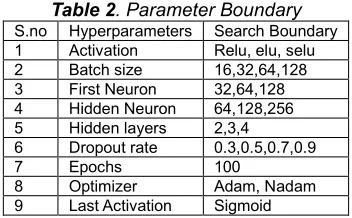
computational cost. The model type is also chosen to be simple neural network with most common/popular hyperparameters. Though complex model that use CNN, RNN, LSTM etc. are present and are used for similar application in other researches. But here a very simple architecture is adopted as concept of proof that such techniques can be used for finding optimal parameters. This may lay foundation brick to use such techniques in finding optimal model for future work in other models in air quality modelling studies as mentioned above. The Flowchart of Talos Scan is shown in figure 2. Here we will list Parameter (dictionary) in Table 2 also known as parameter boundaries used in Talos:
Table 2. Parameter Boundary S.no Hyperparameters Search Boundary 1 Activation Relu, elu, selu 2 Batch size 16,32,64,128 3 First Neuron 32,64,128 4 Hidden Neuron 64,128,256 5 Hidden layers 2,3,4 6 Dropout rate 0.3,0.5,0.7,0.9
7 Epochs 100
8 Optimizer Adam, Nadam 9 Last Activation Sigmoid
The model chosen here is a sequential neural network with some hidden layers and layers have dropout in between them.
Each layer has activation function after it and last layer activation is sigmoid for binary classification. Final layer has one neuron that generate binary output for two classes. With binary_crossentropy as loss function and an optimizer. The model is trained for 100 epochs for each round. Here activation function, batch size, Neuron in each layer, dropout rate, epochs, optimizer etc. is defined for Talos scan here the last Activation function is fixed because of binary classification. Here a limited range of parameter is used to limit the permutation/combination of these parameter and to reduce the scan space of Talos. As increasing the parameter can increase the combination is a non-linear fashion and we also want to limit the cases to a minimum number.
2
REVIEW OF LITERATURE
This part traces the development of literature related to this research. In particular, a brief review of past research for air pollution modelling, is presented so as to provide a perspective for the current work. The literature review is divided into two parts, review of existing Air quality index and current system in India and various researches based on use of machine learning techniques. Research on Developing Air Quality Index (AQI) [1] was not much significantly pursued in India monitoring program started in 1984 till then such programs are non-existent. In Sharma et al [2][3][4] proposed initial and foundation work on formulating a formal AQI and also here max operator is adopted for calculation if AQI from sub-indices. Recently in Beig.et al [5] purposed an evolved AQI model that include more parameters in calculating AQI and also include time characteristics of these pollutants in calculating AQI which was again refreshed in CPCB 2009 to include further parameters to include 12 major and minor pollutants. A Detailed review of different type of Index Proposed by different agencies in given by Kanchan et al [6]. Several Model have been used and proposed by different researchers which uses different machine learning algorithms. Some of the earliest work explore the newly proposed machine learning algorithms and with each subsequent research new methods tries to improve the research in this domain. And such exploration in this domain is necessary to lay down new work in improving the quality of this research. Some of these works is mentioned in this section. Earlier Model for air pollution modelling is based on statistical model [7] for finding a linear relationship between parameters as these models are purely mathematically driven hence sometimes does not perform well as new methods such as artificial neural network are introduced in other fields. It attracted the attention of researchers to implement the algorithms in this domainEarlier applications of the multilayer perceptron (MLP) [8]. Main focus was on the design of MLP, its applications along with a critical analysis of back-propagation algorithm. Implementation of neural networks are found tough to implement and interpret due to some problems. First, the no preceding rules are available to decide the neural architecture, such as nodes in each layer. Second, over fitting the training data resulting in poor generalization. Third, ANN Applications in Air Quality Monitoring and Management back-propagation algorithm in the case of a smaller number of nodes when it cannot be able to converge to a minimum during training. Fourth, curse of dimensionality which affects the speed of back propagation algorithm. To reduce the complexity of NN like feature selection and pattern selection were suggested. So, properly trained MLP still shows the potential to represent Start
Set Search Boundaries in Parameter Dictionary
Configure experiment with arguments
Run the Experiment
Analyze and Evaluate Results
Deploy Model
Accept Model
Stop
Yes
No
1438 relationships, often with surprising accuracy. Research on
―coarse grained Genetic algorithm within Neural Network structure of Multi-layer Perceptron‖ [9] for prediction of next day concentrations for a pollutant is carried out and founded the work for evolutionary computing with ANN. The concentration data with pre-processed meteorological data is used. Missing values are imputed using hybrid methods such as linear interpolation and SOM. the problem is a non-linear regression problem so MLP is used for predicting concentration of next day(T+24h). This MLP Structure is used with Coarse Grained GA to employ parallelism in this evolutionary method. The input parameters optimized using GA where different input parameters are encoded as population of GA and used to tune input parameter of Neural Network but the tuning of control parameter of this evolutionary algorithm is largely an empirical task as one could apply different fitness function to different inputs and form a different result thus this approach is very noisy in nature. To reduce the number of features and better convergence, model using Principal component Analysis [10] is implemented with Multiple linear Regression (MLR) where it performed statistically good and help us to reduce the number of predictor variables. And suggested the idea of reducing the number of features that does not help us in prediction or correlation with the predictor variables are lower.so important pre-processing of data as well as corelated parameters are needed. Hence, we can say Feature Engineering is needed before applying any machine learning algorithm. Similar approaches to augment currently existing using hybridization is introduced subsequently. such as use of Support vector machine (SVM) optimized by Grey Wolf Optimization [11] is used to classify the air quality data and an improved result are found when compared with SVM with kernels linear, nonlinear, polynomial, Gaussian kernel, Radial basis function (RBF), sigmoid etc. which are implemented by Chi-Man Vong et al [12] in a comparative research. Some research is based on ensemble of different machine learning [13]and choose the best result from them such as model that use Artificial neural network (ANN), geographically weighted regression (GWR), the nonlinear autoregressive exogenous Neural Network (NARX), and support vector regression (SVR) is used and best result were selected to improve the overall accuracy of the individual models. Also missing data is interpolated and noisy data is filtered in this research, use of filter such as Sav_gol Filter is proposed to reduce dimensionality and complexity of data. So, we can say a very sophisticated data pre-processing system is used before applying the machine learning algorithm to further enhance the performance of the model. Similarly, many proposed models are implemented that employs different machine learning algorithms. Our thesis is based on use of deep learning neural network, so here will discuss some few applications of deep learning neural network in different domain and air quality prediction in particular. Deep neural networks (DNN) are distinct from other neural networks as the network contain more neuron than previous networks to express complex models, complex connection between layers and more computation power to train and further automatic extraction of the feature. DNN is used mostly in big data researches with exceptional results. Currently DNN are applied in almost all of the machine learning problems such as Compute vision, Recommendation system, pattern identification, Natural language processing etc. [14]. Some of the Deep Learning Neural Network such as deep belief
network. Restricted Boltzmann machine, autoencoder and convolutional neural network has found popularity in industrial and practical application. One of the most common and popular DNN is the convolutional neural network (CNN) as the name suggest these are particularly designed to recognize images as convolution function is inbuilt in these networks. Though other applications have found it ways to use CNN. Study showed excellent performance of CNN in machine learning problems [15]. DNN particularly used in air pollution prediction is new topic of research and the research in still in its infancy so much exploration is not done yet. Some of the implementation of DNN in air pollution is based on Stacked auto encoder (SAE), Recurrent Neural Networks, long short-term memory (LSTM) and CNN which we will discuss below.
X. et al [16] used Stacked autoencoder (SAE) for prediction of air pollution ,where the auto encoder are special neural network which encode a input vector x to y using a function f and tries to reconstruct x using a decoder function g which generally cause some loss 𝐿_𝐻 (𝑥, 𝑧).SAE are autoencoder stacked such that the layer get input from previous layers autoencoder. The research also implemented a special training algorithm [17] that pre-train the network layer by layer in bottom up approach. Finally, the model performed better than Support vector regression (SVR), Autoregressive moving average model (ARMA) and Artificial Neural Network (ANN). The model is evaluated using RSME, MAE and MAPE and always performed better than other model compared in this research. RNN-LSTM was implemented recently by Tsai Y. et al [18] for air pollution prediction where LSTM is used in RNN or LSTM Network. LSTM is a special model where each neuron is also a memory cell and store data and can pass it to next neuron that make them suitable for making RNN. Here PM2.5 is chosen as the predictor variable and predicted for different time interval and the model performance turn out to be excellent however it is observed that the RSME of different station varies much, this can be attributed to some relation between air characteristics between different areas. The prediction shows increase of PM2.5 in future which matches with the actual data. Similarly, a CNN-LSTM is presented by Qin D. et al [19] for prediction of PM 2.5 for data from some Chinese cities with data from 14 monitoring stations. Here CNN is used as an input to the LSTM network, using CNN helps in reduction of parameters and LSTM is able to find correlation between variable easily. This model is compared with competing model such as BP, CNN, LSTM and RNN and these models are evaluated to be least among them by a huge margin which is 14.3% and correlation of 0.97.
3
PROPOSED METHODOLOGY
1439 here the Cumulative index used is based on Indian AQI
system but it is also better in applying a weighted correlation between all sub-indices of major pollutants. The model parameters from Talos are then deployed in a sequential model.
3.1 CUMULATIVE INDEX: AN IMPROVED AQI
The Proposed Model is based on classification of air quality data using a new index required to draw a crisp stratification borderline for air quality considering all pollutants concentrations equally at the same time. So, to generate a borderline for our feature vector. An index is used which is proposed by Yan Wei [11]. The index is called ―cumulative index‖ (CI) and is based on AQI of the pollutants following INAQ, also it does not suffer from eclipsing and ambiguity problem and versatile so that it can be applied for different area and is also not computationally taxing. we have increased the classes from five to six classes to match the current AQI classes in India 𝑅 1, 𝑅 2, 𝑅 3, 𝑅 4, and 𝑅 5, 𝑅 6.The tags associated with the classes is as following and signify the same as the Current AQI system in India
𝑨𝑸𝑰 ∈ 𝑹𝟏 ⇒ 𝒉𝒆 𝒄𝒐 𝒄𝒆 𝒓 𝒊𝒐 𝒊 𝒉𝒆 𝒉𝒚.
𝑨𝑸𝑰 ∈ 𝑹𝟐 ⇒ 𝒉𝒆 𝒄𝒐 𝒄𝒆 𝒓 𝒊𝒐 𝒊 𝒄𝒐 𝒊𝒅𝒆𝒓 𝒃 𝒆.
𝑨𝑸𝑰 ∈ 𝑹𝟑 ⇒ 𝒉𝒆 𝒄𝒐 𝒄𝒆 𝒓 𝒊𝒐 𝒊 𝒉𝒆 𝒉𝒚.
𝑨𝑸𝑰 ∈ 𝑹𝟒 ⇒
𝒉𝒆 𝒄𝒐 𝒄𝒆 𝒓 𝒊𝒐 𝒊 𝒉𝒊𝒈𝒉 𝒚 𝒉𝒆 𝒉𝒚.
𝑨𝑸𝑰 ∈ 𝑹𝟓 ⇒ 𝒉𝒆 𝒄𝒐 𝒄𝒆 𝒓 𝒊𝒐 𝒊 𝒅 𝒈𝒆𝒓𝒐 .
𝑨𝑸𝑰 ∈ 𝑹𝟔 ⇒ 𝒉𝒆 𝒄𝒐 𝒄𝒆 𝒓 𝒊𝒐 𝒊 𝒄𝒓𝒊 𝒊𝒄 .
Now, we calculate CI for different cases where 𝐴𝑄𝐼
belongs to different classes. We employ four major pollutant concentrations (SO2, NO2, PM2.5, and PM10). The value of CI should be such that it increases with the increase in individual pollutant and undergoes sharp increase when more than one pollutant concentrations lie in critical range. The mathematical formulation, which have both the properties and can be used as an improved indicator of air qualityA general classification rule can be identified on the basis of the calculation of this index as proposed by Yan Wei [11] in equation 5 shown below:
𝐶𝐼 =
[
(
( )⁄
)
(
( )⁄
)
(
( )⁄
) .
(
( )⁄
) ( . )
]
(5)
Where 𝑅 & 𝑅 are classes lower and upper bound
respectively and 𝐴𝑄𝐼 are individual sub index of pollutants.
3.2 DATA COLLECTION AND PRE-PROCESSING
Data is collected from ―data.gov.in‖ where dataset from various sectors are provided freely. Here the Historical Air Quality data of Madhya Pradesh for 7 years is compiled from 2004-2011 of 4 major air pollutants namely PM2.5, PM10, NO2 & SO2 etc. Here spatial and meteorological features are not considered and is unavailable to us in this dataset.Figure 4. Dataset
The categorical features are then encoded (label encoder) and all other features are standardized & normalized. Then useless features are dropped such as state, area, date etc. using correlation data. Missing data rows are dropped and outliers are removed using Z-score. Then using the processed data frame, the AQI for all pollutants are calculated and from the AQI, cumulative index and associated label is calculated from it. The research is more focused on binary
classification/prediction of air quality in two classes: Good and Critical so 0 and 1 are adopted as two classes in our target vector. 70% data is used for training and validation and 30 % for testing
1440 Figure 6. Label used for classification and their value count
3.3 Proposed Model
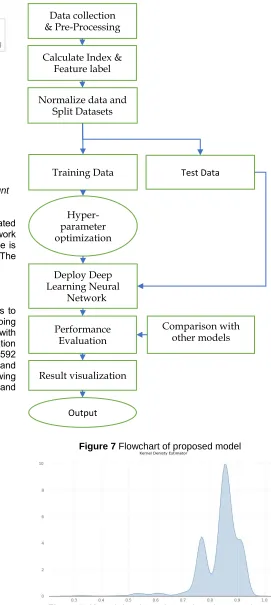
Air quality data is collected for calculating CI and associated Feature label and then Using Deep Learning Neural Network optimized using Talos for Classification and its performance is compared with other machine learning algorithms. The Flowchart in Figure 7 Indicates the Proposed Method
3.4 DEEP LEARNING ARCHITECTURE & HYPERPARAMETER OPTIMIZATION
The Hyperparameter search space is searched using Talos to converge faster model definition have early stopping parameter, also Talos itself provide random search with probabilistic reduction of permutations using correlation method. despite that total number of permutations is 2592 which take about 7 hours and 51 minutes to complete and maximum val_acc model is deployed. After Talos scan following kde plot depicts the scan attributes based on val_acc and val_loss:
Figure 7 Flowchart of proposed model
Figure 7. Kernel density estimator 'metrices = val_acc' Test Data
Data collection & Pre-Processing
Calculate Index & Feature label
Normalize data and Split Datasets
Deploy Deep Learning Neural
Network Hyper-parameter optimization
using Talos
Performance Evaluation
Result visualization
Comparison with other models
Output
1441 Figure 8. Kernel Loss 'metrices = val_loss’
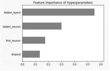
From the above figures it is clear that the max number of models have around 75% to 90 % val_acc and 20% to 35 % val_loss. And a quite a few cross 90% marks, here we are selecting model with best val_acc = 91.12%. Then we have calculated feature importance of hyperparameter, by using the data from scan object from the Talos. here number of hidden layers is most important, followed by number of nodes of hidden layers. Also, if we drop to zero hidden layers, then first layer size become critically important. For each and every scan such correlation can be mapped to further map the relation between hyperparameters.
Figure 9. Feature Importance of Hyperparameter
Further research is need to improve on these results. As the computation is very taxing and our local setup is very inefficient so the scan is done on google Collab with following specification GPU: 1xTesla K80 with 12GB GDDR5 VRAM. CPU: Intel Xeon Processors @2.3Ghz and about 13 GB of ram. For every 12hrs or so Disk, RAM, VRAM, CPU cache etc data that is on their allotted virtual machine will get erased.so longer scan need a longer runtime and even more powerful machine to reduce sec/iteration of the scan
4 RESULT AND DISCUSSION
The optimal values for the parameters and hyperparameters of the DNN, obtained with the Talos scan are shown in Table 4.1.
Table 3 Optimal Hyperparameters S.no Hyperparameters Value
1 First Neuron 128
2 Hidden Layers 3
3 Hidden Neuron 256
4 Dropout rate 0.5
5 Batch size 128
6 Activation Elu
7 Optimizer Adam
The model is deployed using these hyperparameters and evaluated. The problem of overfitting and underfitting is not observed in our model as we can see in our learning curve. In fig 4.2 the learning curve of the model loss and accuracy converge quite well and no major fluctuation is observed. The model shows no substantial gap between validation and training accuracy and loss. Hence our model is not underfitting and overfitting.
Figure 10. Model Accuracy While Training and Testing
Figure 11. Model loss While Training and Testing
The performance of the models is evaluated with metrics including Accuracy, AUC, Precision, Recall, and F1-Score
Table 4 Performance metrices for overall model S.no Metrices
1 F1 score: 0.908808 2 Accuracy: 0.912642 3 Precision: 0.905992 4 Recall: 0.911642 5 ROC AUC: 0.980617
The Classification Report class wise of the model where 0-Good and 1-Critical is depicted below in figure 12.
1442 The Confusion matrix is plotted for test data using the deployed
model
Figure 13. Confusion matrix
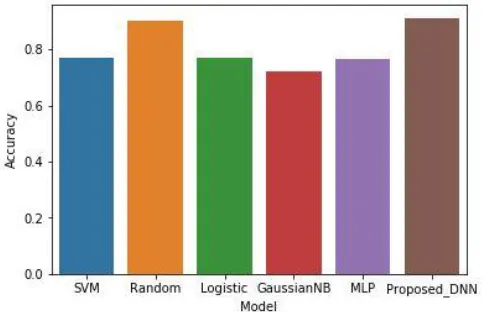
4.1 Comparison with other Models
The model Accuracy is then compared with other classification machine learning algorithm such as SVM, Random Forest, Logistic Regression, Gaussian Naive bayes, MLP etc.
Table 5. Accuracy of different algorithms with proposed model accuracy
S.no Machine Learning algorithm
Accuracy Precision Recall F1score
1 SVM 0.7703 0.7572 0.7879 0.7722 2 Random
Forest
0.9023 0.8970 0.9147 0.9058 3 Logistic
Regression 0.7686 0.7439 0.7941 0.7682 4 Gaussian NB 0.7210 0.6441 0.9428 0.7654 5 MLP 0.7664 0.6801 0.8908 0.7713 6 Proposed
Model
0.9121 0.9059 0.9116 0.9088 The Proposed DNN model performed well as compared with other popular algorithms. The accuracy improvement can be attributed to optimal hyperparameters but the performance is marginal to some algorithm such as random forest where its accuracy is 90.23%. it performed so well that it might be overfitting the data. Other than that, no other machine learning algorithm is comparable to our model.
Figure 14. comparison with other machine learning algorithms
5
CONCLUSION
While the improvement is not substantial but our model performed exceptionally well in contrast to other machine learning algorithms and has scope of improvement despite an
excruciating long hyperparameter search there might be a chance that the hyperparameter chosen in not the best parameter as the probabilistic reduction of the search space is used here. So, it is possible that there might be a model that can perform better than adopted model .Also there is always a possibility that another machine learning technique that will outperform our current model .But here we only try to proof the usefulness of Hyperparameter optimization techniques to implement an optimal model which can be further extended to find hyperparameters for Deep Neural Networks such as CNN,RNN,LSTM etc..
6. FUTURE WORK
A larger dataset is needed for future research. Due to limited data the model perhaps inadequately trained this problem is not unique to our model and other models suffers the same due to limited sample space. As in image classification using machine learning various data augmentation techniques are used but none is featured or present for numerical data other than randomly substituting values, though research is under process to develop such techniques. Also, In future we will improve the analysis of data and try to extend your current model to support multiclass label and prediction of the these classes in a temporal fashion but as of now our approach is limited because of complexity constraints and computational inadequacy in our local setup hence a more powerful and extensive search is need to explore correlation of hyperparameters in model efficiency.
ACKNOWLEDGMENT
I would like to thank my guide Prof. Abhilash Sonker, Dept. of CSE/IT, MITS under his supervision this research is conducted and like to thank him for his guidance during the course of this research, Also I like to thank my friends Prasoon Purwar & Kuldeep Desai (Batch Mate) for their insight suggestions and motivation for this research .They also helped me to revise the manuscript and provide valuable feedback for the same. Although any errors are my own and if any found, I will be only responsible for them.
REFERENCES
[1] Air Quality Index in India, ―The official website of Pollution Control Board of India,‖ http://cpcb.nic.in/. [2] 5.Sharma, M., Maheshwari, M., and Pandey, R.
2001.Development of air quality index for data interpretation and public information. IIT-Kanpur, Report submitted to Central Pollution Control Board Delhi.
[3] 6.Sharma, M., Aggrawal, S, Bose P. (2002). Meteorology-based Forecasting of Air Quality Index using Neural Network. Proceedings of International Conference ICONIP’02-SEAL’02-FSKD’02 on Neural Network, Singapore, November, 2002.
[4] 7.Sharma, M.,Maheshwari, M., Sengupta, B., Shukla B.P. (2003). Design of a website for dissemination of air quality index in India Environmental Modelling & Software 18 (2003) 405–411.
[5] Beig G., Ghude S. D., Deshpande A., Scientific Evaluation of Air Quality Standards and Defining Air Quality index for India, 2010; Indian Institute of Tropical Meteorology-Pune; ISSN 0252-1075.
1443 Atmospheric Environment, volume 9, no.2,pp.101–
113,2015.
[7] Shi, J. P. and R.M. Harrison (1997): Regression modelling of hourly NOx and NO2 concentrations in urban air in London. Atmospheric Environment, 31, pp. 4081-4094.
[8] Gardner, M. W. and Dorling, S. R. (1998): Artificial neural networks (the multilayer perceptron) – a review of applications in the atmospheric sciences. Atmospheric Environment, Vol. 32, No. 14/15, pp. 2627-2636.
[9] Niska H, Hiltunen T, Karppinen A, Ruuskanen J, Kolehmainen M. Evolving the neural network model for forecasting air pollution time series. Eng Appl Artif Intell. 2004:159–167
[10]Kumar and P. Goyal, ―Forecasting of air quality in Delhi using principal component regression technique,‖ Atmospheric Pollution Research, vol.2, no.4, pp.436–444,2011.
[11]Yan Wei, Ni Ni, Dayou Liu, et al., ―An Improved Grey Wolf Optimization Strategy Enhanced SVM and Its Application in Predicting the Second Major,‖ Mathematical Problems in Engineering, vol. 2017, Article ID 9316713, 12 pages, 2017.
[12]Chi-Man Vong, Weng-Fai Ip, Pak-kin Wong, and Jing-yi Yang, ―Short-Term Prediction of Air Pollution in Macau Using Support Vector Machines,‖ Journal of Control Science and Engineering, vol. 2012, Article ID 518032, 11 pages, 2012
[13]Delavar, M.R.; Gholami, A.; Shiran, G.R.; Rashidi, Y.; Nakhaeizadeh, G.R.; Fedra, K.; Hatefi Afshar, S. A Novel Method for Improving Air Pollution Prediction Based on Machine Learning Approaches: A Case Study Applied to the Capital City of Tehran. ISPRS Int. J. Geo-Inf. 2019, 8, 99.
[14]W. Liu, Z. Wang, X. Liu, N. Zeng, Y. Liu, F.E. Alsaadi, A survey of deep neural network architectures and their applications, Neurocomputing 234 (2017) 11e26. [15]S. Albawi, T.A. Mohammed, S. Al-Zawi, Understanding of a convolutionalneural network, in: International Conference on Engineering and Technology (ICET), IEEE, 2017, pp. 1e6.
[16]Li, Xiang & Peng, Ling & Hu, Yuan & Shao, Jing & Chi, Tianhe. (2016). Deep learning architecture for air quality predictions. Environmental Science and Pollution Research. 23. 10.1007/s11356-016-7812-9. [17]Hinton GE E., Osindero S, and Teh YW. 2006. A fast
learning algorithm for deep belief nets. Neural Comput. 18, 7 (July 2006), 1527-1554.
[18]Y. Tsai, Y. Zeng and Y. Chang, "Air Pollution Forecasting Using RNN with LSTM," 2018 IEEE 16th Intl Conf on Dependable, Autonomic and Secure Computing, 16th Intl Conf on Pervasive Intelligence and Computing, 4th Intl Conf on Big Data Intelligence and Computing and Cyber Science and Technology Congress (DASC/PiCom/ DataCom/CyberSciTech), Athens, 2018, pp. 1074-1079.
[19]D. Qin, J. Yu, G. Zou, R. Yong, Q. Zhao and B. Zhang, "A Novel Combined Prediction Scheme Based on CNN and LSTM for Urban PM2.5 Concentration," in IEEE Access, vol.7, pp.20050-20059, 2019.doi: 10.1109/ACCESS.2019.2897028
[20]Franois Chollet, ―Keras,‖ 2016. [Online]. Available: https://keras.io/