Vol. 13 (2019) 3254–3296 ISSN: 1935-7524
https://doi.org/10.1214/19-EJS1608
Multiscale change-point segmentation:
beyond step functions
Housen Li †,∗ Qinghai Guo† and Axel Munk†,‡
University of G¨ottingen†and Max Planck Institute for Biophysical Chemistry‡ G¨ottingen, Germany
e-mail:[email protected];[email protected];[email protected]
Abstract: Modern multiscale type segmentation methods are known to detect multiple change-points with high statistical accuracy, while allow-ing for fast computation. Underpinnallow-ing (minimax) estimation theory has been developed mainly for models that assume the signal as a piecewise constant function. In this paper, for a large collection of multiscale seg-mentation methods (including various existing procedures), such theory will be extended to certain function classes beyond step functions in a nonparametric regression setting. This extends the interpretation of such methods on the one hand and on the other hand reveals these methods as robust to deviation from piecewise constant functions. Our main find-ing is the adaptation over nonlinear approximation classes for a universal thresholding, which includes bounded variation functions, and (piecewise) H¨older functions of smoothness order 0< α≤1 as special cases. From this we derive statistical guarantees on feature detection in terms of jumps and modes. Another key finding is that these multiscale segmentation methods perform nearly (up to a log-factor) as well as the oracle piecewise con-stant segmentation estimator (with known jump locations), and the best piecewise constant approximants of the (unknown) true signal. Theoretical findings are examined by various numerical simulations.
MSC 2010 subject classifications:62G08, 62G20, 62G35.
Keywords and phrases:Change-point regression, adaptive estimation, oracle inequality, jump detection, model misspecification, multiscale infer-ence, approximation spaces, robustness.
Received January 2019.
1. Introduction
Throughout we assume that observations are given through the regression model
yin= ¯fin+ξni, i= 0, . . . , n−1, (1) where ¯ fin =n [i/n,(i+1)/n) f0(x)dx , (2) and ξn = (ξn
0, . . . , ξnn−1) are independent (not necessarily i.i.d.) centered
sub-Gaussian random variables with scale parameterσ, that is,
Eeuξni
≤eu2σ2/2, for everyu∈R. ∗Corresponding author.
3255
For simplicity, the scale parameter σ in model (1) is assumed to be known. In fact, if the noise distribution is known, say Gaussian, σ can be easily pre-estimated√n-consistently from the data via local differences (see e.g. M¨uller and Stadtm¨uller,1987; Hall and Marron,1990; Munk et al.,2005; Tecuapetla-G´omez and Munk, 2017). For the general sub-Gaussian case, estimation of σ is not obvious, but the missing knowledge ofσwill actually not affect our asymptotic results (cf. Remark3), as only an upper bound ofσ is needed.
In this paper we are concerned with potentially discontinuous signals f0 :
[0,1)→Rin (2). As a minimal condition, we always assume that the underly-ing (unknown) signal f0 lies in D ≡ D([0,1)), the space of c`adl`ag functions
on [0,1), which are right-continuous and have left-sided limits (cf. Billings-ley, 1999, Chapter 3). In (2), we embed for simplicity the sampling points
xi,n=i/nequidistantly in the unit interval. However, we stress that all our re-sults can be transferred to more general domains (⊆R) and sampling schemes, also for random xi,n. For technical simplicity, we consider local averages ¯fin in model (1). The difference to point evaluation is asymptotically ignorable, since limn→∞n
[x,x+1/n)f(t)dt = f(x) forx ∈ [0,1) and f ∈ D. In many
applica-tions, e.g., nuclear magnetic resonance spectroscopy (Spraul et al., 1994), the local averages (a.k.a. data binning) are the typical measurements.
For the particular case thatf is piecewise constant with a finite but unknown number of jumps, model (1) has been of particular interest throughout the past and is often referred to as change-point regression model. The related problem of estimating the number, locations and sizes of change-points (i.e. its loca-tions of discontinuity) has a long and rich history in the statistical literature. Tukey (1961) already phrased the problem of segmenting a data sequence into constant pieces as the “regressogram problem” and it occurs in a plenitude of applications. From a risk minimization point of view it is well known that cer-tain Bayesian estimators are (asymptotically) optimal (see e.g. Ibragimov and Has’minski˘ı (1981, Chapter VII) and Korostelev and Korosteleva (2011, Chap-ter 5)); however, they are not easily accessible from a computational point of view, particularly when it comes to multiple change-point recovery (Antoch and Huˇskov´a,2000). Therefore, recent years have witnessed a renaissance in change-point inference motivated by several applications which requirecomputationally fast andstatistically efficientfinding of potentiallymanychange-points in large data sets, see e.g. Olshen et al. (2004), Siegmund (2013) and Behr, Holmes and Munk (2018) for its relevance to cancer genetics, Chen and Zhang (2015) for network analysis, Aue et al. (2014) for econometrics, and Hotz et al. (2013) for electrophysiology, to name a few. A major challenge for statistical methodology is the multiscale nature of these problems (i.e. change-points occur at differ-ent e.g. temporal scales and their number can be potdiffer-entially large) and the large number of data points (a few millions or more), requiring computationally efficient methods.
Such computationally efficient segmentation methods which provide at the same hand certain statistical guarantees for their findings are either based on dy-namic programming (Boysen et al., 2009; Killick, Fearnhead and Eckley, 2012;
3256
Frick, Munk and Sieling, 2014; Du, Kao and Kou, 2016; Li, Munk and Siel-ing, 2016; Maidstone et al.,2016; Haynes, Eckley and Fearnhead, 2017), local search (Scott and Knott, 1974; Olshen et al., 2004; Fryzlewicz,2014; Fang, Li and Siegmund,2019) or convex optimization (Harchaoui and L´evy-Leduc,2008; Tibshirani and Wang,2008; Harchaoui and L´evy-Leduc,2010) resulting from a convex1 relaxation of the combinatorial0 search problem of the best fitting
change-points.
Typically, the statistical justification for all the aforementioned methods is given for models which assume that the underlying truth is a piecewise con-stant function with a fixed but unknown number of changes. For extensions to increasing number of changes of the truth (as the number of observations in-creases), see e.g. Zhang and Siegmund (2012), Frick, Munk and Sieling (2014) and Fryzlewicz (2014), or Cai, Jeng and Li (2012) under an additional sparsity assumption. However, in general, nothing is known for such segmentation meth-ods in the general nonparametric regression setting as in (1) when f is not a piecewise constant function, e.g. a smooth function. Notable exceptions are the jump-penalized least square estimator in Boysen et al. (2009), and the unbal-anced Haar wavelets based estimator in Fryzlewicz (2007), for which theL2-risk
has been analyzed for functions which can be sufficiently fast approximated by piecewise constant functions (in our notation this corresponds to functions in the spaceAγ2, see section3.2 for the definition).
Intending to fill such a gap, we provide a comprehensive risk analysis for a range of multiscale change-point methods whenf in (1) is not a change-point function a priori. To this end, we introduce in a first step a general class of
multiscale change-point segmentation (MCPS) methods, with scales specified by generalc-normal systems (adopted from Nemirovski (1985), see Definition 1), unifying several previous methods. This includes particularly the simultane-ous multiscale change-point estimator (SMUCE) by Frick, Munk and Sieling (2014) which minimizes the number of change-points under a side constraint that is based on a simultaneous multiple testing procedure on all scales (length of subsequent observations). Further examples are estimators which are built on different multiscale systems (Walther, 2010), or multiscale type penalties (Li, Munk and Sieling,2016). These methods can be viewed also as a natural mul-tiscale extension of certain jump penalized estimators via convex duality (see Boysen et al.,2009; Killick, Fearnhead and Eckley,2012). Implemented by accel-erated dynamic programming algorithms, these methods often have a runtime
O(nlogn), and are found empirically promising in various applications (see e.g. Hotz et al.,2013; Futschik et al.,2014; Behr and Munk,2017; Killick, Fearnhead and Eckley,2012). In case thatf in model (1) is a step function, the statistical theory for these methods is well-understood meanwhile. For example, minimax optimality of estimating the change-point locations and sizes has been shown, which is based on exponential deviation bounds on the number, and the loca-tions of change-points. Furthermore, these methods also obey optimal minimax detection properties (in the sense of testing) of vanishing signals, and provide simultaneous confidence statements for all unknown quantities (see Frick, Munk and Sieling,2014; Li, Munk and Sieling, 2016; Pein, Sieling and Munk,2017).
3257
To complement the understanding of such methods, this work aims to ana-lyze their behavior when the true regression function f0 is beyond a piecewise
constant function. To this end, we derive convergence rates for sequences of piecewise constant functions with increasing number of changes (Theorem 1), and for functions in certain approximation spaces (Theorem2), well-known in approximation theory, cf. DeVore and Lorentz (1993, Chapter 12), (see Sec-tion 3). Further, we generalize the above mentioned results for quadratic risk to general Lp-risk (0 < p < ∞). As a consequence, we obtain the minimax optimal ratesn−2/3·min{1/2,1/p}andn−2α/(2α+1)(up to a log-factor) in terms of
Lp-loss both almost surely and in expectation for the cases thatf has bounded variation (0 < p < ∞) (see Mammen and van de Geer, 1997), and that f is (piecewise) H¨older continuous of order 0 < α ≤ 1 (0 < p ≤ 2), respectively. Most importantly, the discussed MCPS methods are universal (i.e. indepen-dent of the smoothness assumption of the unknown truth signal), as the only tuning parameter η (which serves as a threshold, see Section 2 for further de-tails) can be chosen as η √logn. We will show that for this choice, these methods automatically adapt to the unknown “smoothness” of the underlying function in an asymptotically optimal way, no matter whether it is piecewise constant or it lies in the aforementioned function spaces. As an illustration, we present the performance of SMUCE (Frick, Munk and Sieling, 2014) with universal parameter choiceη = 0.42√logn, on different signals in Figure 1. It clearly shows that SMUCE, although designed to provide a piecewise constant solution, successfully recovers the shape of all underlying signals no matter whether they are locally constant or not, as suggested by our theoretical find-ings.
Further, the developed theory allows us to derive statistical guarantees for fea-ture detection, see Section4. More precisely, we show for general (incl. piecewise constant) signals in approximation spaces that the discussed methods recover at least as many jumps and modes (or troughs) as the truth, as the sample size tends to infinity (Theorem 3); This statement should be interpreted with the built-in parsimony (i.e., minimization of number of jumps) of these methods, which suggests that the number of artificial jumps and modes (or troughs) is “minimal”. At the same hand, large increases (or decreases) of the discussed estimators imply increases (or decreases) of the true signal with high confidence (Theorem 4). In Figure 2, based on our theoretical finding, one can claim, for example, that the two large jumps (marked by solid vertical lines) are signifi-cant with confidence at least 90% (see Remark8). In the particular case of step signals, we further show the consistency in estimating the number of jumps, and an error bound of the best known order (in terms of sample sizes) on the estimation accuracy of change-point locations (Proposition1).
Finally, we address the issue how to benchmark properly the investigated methods. We show that the MCPS methods with a universal threshold per-form nearly no worse than piecewise constant segmentation estimators whose change-point locations are provided by an oracle. By considering such oracles, we discover asaturation phenomenon (Theorem5and Example 2) for the class of all piecewise constant segmentation estimators: only the suboptimal raten−2/3
3258
Fig 1. Estimation by the multiscale change-point segmentation method SMUCE (Frick, Munk
and Sieling, 2014) for Blocks, Bumps, Heavisine, and Doppler signals (Donoho and John-stone,1994) with sample sizen=1,500, and signal-to-noise ratiofL2/σ= 3.5.
is attainable for smoother functions in H¨older classes with smoothness order
α >1. From a slightly different perspective, we show that the MCPS methods perform nearly as well as the best (deterministic) piecewise constant approxi-mant of the true signal with the same number of jumps or less (Proposition2). Besides such theoretical interest (cf. also Linton and Seo, 2014; Farcomeni,
2014), the study of these estimators in models beyond piecewise constant tions is also of particular practical importance, since a piecewise constant func-tion is actually known to be only an approximafunc-tion of the underlying signal in many applications. For example, in DNA copy number analysis, for which the change-point regression model with locally constant signal is commonly assumed (see e.g. Olshen et al., 2004; Lai et al., 2005), a periodic trend dis-tortion with small amplitude (known as genomic waves) is well known to be present (Diskin et al.,2008). Thus our work can be also regarded as examination of the robustness of such segmentation methods against model misspecification.
3259
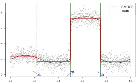
Fig 2. Feature detection by SMUCE with threshold η(0.1) by (7)(sample size n = 1,000,
SNR= 5). The solid vertical lines mark significant jumps, while the dashed one marks an insignificant jump; and the arrows at the bottom indicate significant increases and decreases; with simultaneous confidence at least90%. See Remark8in Section4for details.
We consider a piecewise constant estimator as robust, if it recovers the majority of interesting features of the underlying true regression function with as small number of jumps as possible. For instance, Figure 3 shows the performance of SMUCE on a typical signal from DNA copy number analysis, where a locally constant function is slightly perturbed, in cases of different noise levels. Visually, SMUCE seems to recover the major features, and the recovered signal provides a simple yet informative summary of the data, meanwhile staying close to the true signal, which confirms our theoretical findings. We note that our viewpoint here complements a recent work by Song, Banerjee and Kosorok (2016) who considered areversescenario: a sequence of smooth functions approaches a step function in the limit.
In summary, we show that a large class of multiscale change-point segmenta-tion methods with a universal parameter choice areadaptively minimax optimal
(up a log-factor) for step signals (possibly with unbounded number of change-points) and for (piecewise) smooth signals in certain approximation spaces (The-orems 1 and 2) with respect to general Lp-risk. Building on this, we obtain statistical guarantees on feature detection, such as recovery of the number of discontinuities, or modes (Proposition1and Theorems3and4), which explain well-known empirical findings. Moreover, in the particular case ofL2 distance, we show oracle inequalities for such multiscale change-point segmentation meth-ods in terms of both segmentation and approximation of the true signal (Theo-rem5 and Proposition2).
The paper is organized as follows. In Section2, we introduce a general class of multiscale change-point segmentation methods, discuss examples and
pro-3260
Fig 3. Estimation by SMUCE with threshold η(0.1) for the signal in Olshen et al. (2004)
and Zhang and Siegmund (2007) with various signal-to-noise ratiosfL2/σ, cf. Section6.
vide technical assumptions. We derive uniform bounds on theLp-loss over step functions with possibly increasing number of change-points and over certain approximation spaces in Section3, and present their implication on feature de-tection in Section 4. Section 5 focuses on the oracle properties of multiscale change-point segmentation methods from a segmentation and an approxima-tion perspective, respectively. Our theoretical findings are investigated for finite samples by a simulation study in Section 6. The paper ends with a conclusion in Section7. Technical proofs are collected in the appendix.
2. Multiscale change-point segmentation
To ease presentation, we introduce some notation. Forx, y∈R, let
x∧y:= min{x, y}, x∨y:= max{x, y} and (x)+:=x∨0.
Recall model (1) and let f now in S ≡ S([0,1)), the space of right-continuous step functions f on [0,1) with a finite (but possibly unbounded) number of
3261
jumps, that is, for somek∈N f =
k
i=0
ci1[τi,τi+1) with 0 =τ0< . . . < τk+1= 1, andci=ci+1 for alli. (3) HereJ(f) :={τ1, . . . , τk}denotes the set of change-points off. Byintervalswe always refer to those of the form [a, b), 0≤a < b≤1. In the following we in-troduce a general class of multiscale change-point estimators comprising various methods recently developed. To this end, we fix a system I of subintervals of [0,1) in the first step (cf. Definition1). GivenI, we introduce a general class of
multiscale change-point segmentation (MCPS) estimators ˆfn (see Frick, Munk and Sieling,2014; Li, Munk and Sieling,2016; Pein, Sieling and Munk,2017) as a solution to the (nonconvex) optimization problem
min f∈S#J(f) subject toTI(y n;f)≤η. (4) Here yn := {yn i} n−1
i=0 is the observational vector, and η ∈ R is a threshold to
be defined later. As a convention, we consider in (4) only those candidate func-tionsf whose change-points lie on the grid{i/n}n
i=0. The side constraint in (4)
is defined by a multiscale test statistic
TI(yn;f) := max I∈I f≡cIonI ⎧ ⎨ ⎩ 1 n|I| i/n∈I (yin−cI)−sI ⎫ ⎬ ⎭, (5)
with sI ∈Ra scale penalty, which can be deterministic or random, and might even depend on the candidatef and the datayn. The maximum in (4) is taken over all intervalsI∈ I, on which the candidate functionf is constant. We will assume thatη+sI ≥0 for allI∈ I, see Definition2. In this case, the constraint in (4) is not empty, as it containsf =ni=0yn
i1[i/n,(i+1)/n). Thus, the solution
to the optimization problem (4) always exists but might benon-unique, in which case one could pick an arbitrary solution.
The side constraint in (4) originates from testing simultaneously the residuals of a candidatef with valuescI on the multiscale systemI. In model (1) under a Gaussian error, this combines all the local likelihood ratio tests whether the local mean off0onIequals to a givencI for everyI∈ I. Hence, this provides a cri-terion for testing the constancy off0on each of its segments inI (for a detailed
account see Frick, Munk and Sieling,2014). The choice of the scale penaltiessI determines the estimator. It balances the detection power over different scales, see D¨umbgen and Spokoiny (2001), Walther (2010) and Frick, Munk and Siel-ing (2014) for several choices, and Davies, H¨ohenrieder and Kr¨amer (2012) for the unpenalized estimators (i.e.sI ≡0) in a slightly different model. Thus, any MCPS method amounts to search for the most parsimonious candidate over the acceptance region of the multiple tests on the right hand side in (4) performed over the systemI. The thresholdη in (4) provides a trade-off between data-fit and parsimony, and can be chosen such that the truthf0 satisfies the side
3262
the (1−β)-quantile of the distribution ofTI(ξn; 0), which can be determined by Monte-Carlo simulations or asymptotic considerations (Frick, Munk and Siel-ing, 2014; Pein, Sieling and Munk, 2017). Then the choice of significance level
β provides an upper bound on the family-wise error rate of the aforementioned multiple test. It immediately provides for ˆfn a control of overestimating the number of jumps #J(f0) off0, i.e.
P#J( ˆfn)≤#J(f0)
≥1−β uniformly over allf0∈ S.
Also, with a different penalty, it is possible to control instead the false discovery rate by means oflocal quantiles, see Li, Munk and Sieling (2016) for details. We will see that for the asymptotic analysis of all these estimators it is sufficient to work with a universal threshold η √logn in (4) (see Definition 2 and Section3).
The systemI will be required to be trulymultiscale, i.e. the MCPS methods in (4) require the associated interval system I to contain different scales, the richness of which can be characterized by the concept ofnormality.
Definition 1 (Nemirovski (1985)). A system I ≡ In of intervals is called
normal (or c-normal) for some constant c > 1, provided that it satisfies the following requirements.
(i) For every intervalI ⊆[0,1) with length |I|> c/n, there is an interval ˜I
in I such that ˜I⊆I and|I˜| ≥c−1|I|.
(ii) The end-points of each interval inIlie on the grid{i/n:i= 0, . . . , n−1}. (iii) The systemI contains all intervals [i/n,(i+ 1)/n),i= 0, . . . , n−1.
Remark 1 (Normal systems). The requirement (i) in the above definition is crucial, while (ii) and (iii) are of technical nature due to the discrete sampling locations{i/n}ni=0−1and can be generalized. Examples of normal systems include the highly redundant systemI0of all intervals whose end-points lie on the grid
{i/n}ni=0−1(suggested by e.g. Siegmund and Yakir,2000; D¨umbgen and Spokoiny,
2001; Frick, Munk and Sieling, 2014) of order O(n2), and less redundant but
still asymptotically efficient systems (Davies and Kovac, 2001; Walther, 2010; Rivera and Walther,2013), typically of orderO(nlogn). Remarkably, there are even normal systems with cardinality of orderO(n), such as thedyadic partition system i n2 −jn,i+ 1 n 2 −jn:i= 0, . . . ,2j−1, j= 0, . . . ,log 2n ,
which can be shown to be 2-normal, see Grasmair, Li and Munk (2018). We further stress that the choice ofI in general poses no restriction on the change-point locations of solutions to (4), which is in sharp contrast to the wavelet thresholding approaches (e.g. Abramovich, Antoniadis and Pensky, 2007) and the local/reverse segmentation approach by Chan and Chen (2017).
Definition 2(Multiscale change-point segmentation estimator). Any estimator satisfying (4) is denoted as a multiscale change-point segmentation (MCPS) estimator, if
3263
(i) the interval systemI isc-normal for some constantc >1; (ii) the scale penaltiessI satisfy almost surely that
max I∈I|sI| ≤δ
logn for some constantδ >0.
(iii) the thresholdη is chosen as
η=alogn witha > δ+σ√2r0+ 4, (6)
for some fixedr0∈(0,∞).
Remark 2 (Scale penalization). For sub-Gaussian errorξn max I∈I 1 n|I| i/n∈I ξin
is at most of order√logn(see e.g. Shao,1995, Theorem 1), so Definition2(ii) is quite natural. In particular, Definition2(ii) includes many common scale penal-ties. For instance, SMUCE (Frick, Munk and Sieling, 2014) and FDRSeg (Li, Munk and Sieling,2016) are special cases. More precisely, for SMUCE, it amounts to select I = I0, the system of all possible intervals, and s
I =
2 log(e/|I|), and for FDRSeg, the same system I =I0 but a different scale penalty s
I =
2 log(e|I0|/|I|) with I0 being the constant segment, which contains I, of the
candidate solution. The case sI ≡ 0 is also included and has been suggested by Davies, H¨ohenrieder and Kr¨amer (2012).
Remark 3(Choice of thresholdη). Note that the choice of the only parameter
η in Definition2 (iii) is completely independent of the unknown truthf0, while
it depends on the distribution of the noiseξnvia the scale parameterσ. In fact, it is also possible to chooseη independent ofξn byη=bn
√
lognwithbn → ∞ arbitrarily slow (e.g.bn= log logn); This will lead to a factorbn in front of the convergence rates in later sections.
Alternatively, as mentioned earlier, we recommend to choose
η=η(β) the (1−β)-quantile ofTI(ξn; 0), (7) withβ =βn∈(0,1), such that
P{TI(ξn; 0)> η(β)−O(1)} ≤ O(n−r0). (8) By Shao’s theorem (Shao,1995, Theorem 1), it then holds that
η(β)≤(δ+σ√2)logn+O(1)≤(δ+ 2σ)logn (9) for large enoughn. To ease presentation, we will state and prove our theoretical results forηgiven in (6), and emphasize that all the results also hold forηgiven in (7), the proofs of which are essentially the same (thus omitted) but relying on (8) and (9) instead. In addition, we note that a more refined analysis ofη(β)
3264
is even possible, although not necessary for our purposes. For instance, in case of no scale penalization, standard Gaussian noise and I =I0 consisting of all
intervals, it follows from Kabluchko (2007, Theorem 1.3) that
η(β)∼2 logn+log logn+ log λ
4π−2 log log(1/β)
2√2 logn asn→ ∞,
with constant λ∈(0,∞), see also Siegmund and Venkatraman (1995, Proposi-tion 1) for approximaProposi-tion ofη(β) for finite sample sizes.
3. Asymptotic error analysis
This section mainly provides convergence rates of the MCPS methods for the model (1).
3.1. Convergence rates for step functions
We consider first locally constant change-point regression, i.e. the underlying signalf0∈ S in model (1). We introduce the class of uniformly bounded
piece-wise constant functions, cf. (3), with up tokjumps
SL(k) :=
f ∈ S: #J(f)≤k, andfL∞ ≤L
,
for k ∈N0 and L ∈(0,∞). If the number of change-points is bounded, i.e. k
is known beforehand, the estimation problem is, roughly speaking, paramet-ric, by interpreting change-point locations and function values as parameters. A rather complete analysis of this situation is provided either from a Bayesian viewpoint (see e.g. Ibragimov and Has’minski˘ı,1981; Huˇskov´a and Antoch,2003, Chapter VII) or from a likelihood viewpoint (see e.g. Yao and Au (1989); Braun, Braun and Mueller (2000); Siegmund and Yakir (2000); Boysen et al. (2009) and Korostelev and Korosteleva (2011, Chapter 5)). However, in order to un-derstand the increasing difficulty of change-point estimation as the number of change-points gets larger, i.e. the nonparametric nature of change-point regres-sion, we allow now the number of change-points to increase as the number of observations tends to infinity.
Theorem 1 (Adaptation I). Assume model (1). Let0< p <∞, andkn ∈N0
be such thatkn=o(n)asn→ ∞. Then:
(i) For any multiscale change-point segmentation estimatorfˆnin Definition2
with somer0∈(0,∞), the following upper bound holds for eachr∈(0, r0]
lim sup n→∞ 1 √ logn n kn+ 1 1/2∧1/p sup f0∈SL(kn) Efˆn−f0r Lp 1/r <∞.
3265
(ii) If noiseξn
i in model (1) has a densityϕi,n such that for some constants
σ0 andz0
max i,n
ϕi,n(x) log ϕi,n(x)
ϕi,n(x+z)dx≤
z2 σ2 0
for|z| ≤z0 (10)
then the following lower bound holds for eachr∈(0,∞)
lim inf n→∞ n kn+ 1 1/2∧1/p inf ˆ gn sup f0∈SL(kn) E[gˆn−f0rLp]1/r>0,
where the infimum is taken over all estimatorsgˆn.
Proof. See AppendixA.1.
Remark 4.
(i) The condition (10) is a typical assumption for establishing lower bounds (see e.g. Tsybakov, 2009, Section 2.5). If exp(−c1x2) ϕi,n(x)
exp(−c2x2) with constants c1, c2, then (10) holds for any z0 > 0, e.g. a
Gaussian density. Note that the universal threshold η in (6) is indepen-dent of the truthf0 and the specific loss function ·Lp for 0 < p < ∞.
The restriction ofr≤r0 is mainly due to control the r-th moment of the
noise, which is quite natural. In most cases, one is interested inr= 1 or 2, for which it is sufficient to setr0= 2. Thus, Theorem1states that the
MCPS estimators are up to a log-factor adaptively minimax optimal over sequences of classesSL(kn) for all possiblekn andL.
(ii) Theorem1 also reveals that the underlying difficulty in estimation of step functions with respect toLp-loss is actually determined by the number of change-points. A common choice ofkniskn nθ, 0≤θ <1, which in par-ticular reproduces the convergence results in Li, Munk and Sieling (2016, Theorem 3.4) but now under weaker assumptions (here no assumption on the minimal segment length and the minimal jump size is made). It also includes the caseθ= 0, where, by convention,kn≡kis bounded.
(iii) Note further that the restrictionp <∞in Theorem1is necessary and nat-ural, becauseL∞-loss is not reasonable in change-point estimation prob-lems (as no estimator can detect change-point locations at a rate faster thanO(1/n), see Chan and Walther,2013, which leads to inconsistency of any estimator with respect toL∞-loss).
(iv) In general, it is not clear whether the lower bound in Theorem 1 (ii) is sharp or not. However, in the particular case thatf0∈ SL(kn) is isotonic, it has recently been shown that the minimax rate in terms of squaredL2
risk is exactly of ordern−1k
nlog logn, see Gao, Han and Zhang (2019).
3.2. Robustness to model misspecification
As discussed in Section 1, in practical applications, it often occurs that the underlying signalf0in model (1) is only approximately piecewise constant. To
3266
address this issue, we next consider theLp-loss of the MCPS methods for more general functions. In order to characterize the degree of model misspecification, we adopt from nonlinear approximation theory (cf. DeVore and Lorentz, 1993; DeVore,1998) theapproximation spaces as
Aγ q := f ∈ D: sup k∈Nk γΔ q,k(f)<∞ , for 0< q≤ ∞,0< γ <∞,
where the approximation error Δq,kis defined as Δq,k(f) := inf
f−gLq :g∈ S, #J(g)≤k
. (11)
Introduce the subclasses
Aγ q,L:= f ∈ D: sup k≥1 kγΔq,k(f)≤L, andfL∞ ≤L ,
for 0 < q ≤ ∞, and 0< γ, L <∞. The best approximant in (11) exists, but is in general non-unique, see e.g., DeVore and Lorentz (1993, Chapter 12). It follows readily from definition that Aγ
q = L>0A γ q,L and that A γ q1,L ⊆ A γ q2,L for allq1≥q2. Note thatAγq is actually an interpolation space betweenLq and some Besov space (see Petrushev, 1988, Corollary 2.2). The order γ of these spaces (or classes) reflects the speed of approximation off by step functions as the number of change-points increases. It is further known that if f lies inAγ q for someγ >1 and iff is piecewise continuous, thenf is piecewise constant, see Burchard and Hale (1975) (which is often referred to as a saturation result in the approximation theory community). Thus, it is custom to considerAγ
q with 0< γ≤1.
The rates of convergence for approximation classes are provided below.
Theorem 2 (Adaptation II). Let 0 < p < ∞, p∨2 ≤ q ≤ ∞, and assume thatfˆn is an MCPS estimator in Definition2with somer0∈(0,∞). Then, for
0< r≤r0 and0< γ, L <∞, lim sup n→∞ (logn) −γ+(1/2−1/p)+ 2γ+1 n 2γ 2γ+1(1/2∧1/p) sup f0∈Aγq,L Efˆn−f0r Lp 1/r <∞.
The same result also holds almost surely if we drop the expectationE[·]. Proof. See AppendixA.2.
Remark 5. Similar to Theorem 1, the above theorem shows that any MCPS method automatically adapts to the smoothness of the approximation spaces, in the sense that it has a faster rate for larger γ. Note that such convergence rates inLp-loss, 0< p≤2, are nearly (i.e. up to a log-factor) minimax optimal over Aγq,L for every 0 < γ ≤1, 2 ≤ q ≤ ∞ and L > 0, since n−γ/(2γ+1) are known to be minimax rates for a smaller class HLγ, see Example 1 (i) below. We conjecture that the convergence rates in Theorem2are also nearly minimax
3267
optimal for Aγq,L with respect toLp-loss when 2< p≤q ≤ ∞, because this is indeed the case forγ= 1, as shown later in Example1 (ii).
Moreover, note that the convergence rates of the MCPS methods above gen-eralize the rates reported in Boysen et al. (2009) for jump-penalized least square estimators, and are faster than the rates reported in Fryzlewicz (2007) for the unbalanced Haar wavelets based estimator, with the difference being in log-factors.
Example 1. (i)(Piecewise) H¨older functions. For 0< α≤1 andL∈(0,∞), we consider the H¨older function classes
HLα≡HLα([0,1)) :=f ∈ D:fL∞ ≤L, and
|f(x1)−f(x2)| ≤L|x1−x2|αfor allx1, x2∈[0,1)
,
and the piecewise H¨older function classes with at most κjumps,κ∈N0
Hκ,Lα ≡Hκ,Lα ([0,1)) :=
f ∈ D: there is a partition {Ii}li=0, withl≤κ, of [0,1)
such thatfI
i ∈H
α
L(Ii) for all possiblei
.
Obviously, the latter one contains the former as a special case whenκ= 0, that is,Hα
0,L≡HLα. By considering step functions with segments of equal length, one can easily show thatHα
L ⊆ Aαq,L with finiteL ≥L and 0< q ≤ ∞, and in a
similar way thatHα
κ,L⊆ Aαq,L with finiteL ≥L(κ+ 1)α+1/2 and 0< q≤ ∞. It is known that the fastest possible rate over Hα
L, 0 < α ≤1, is of order
n−α/(2α+1) with respect to the Lp-loss, 0< p < ∞, see e.g. Nemirovski (2000, Theorem 3.1). Thus, as a consequence of Theorem 2, the MCPS methods are simultaneously minimax optimal (up to a log-factor) over Aαq,L,HLα and Hκ,Lα
for every κ ∈ N0, 0 < p ≤ 2 ≤ q ≤ ∞, 0 < α ≤1 and L ∈ (0,∞), that is,
adaptive to the smoothness order αof the underlying function. The difference in convergence rates forLp-loss, 2 < p <∞, is mainly because Aα
q,Lis strictly larger than Hα
L, see the next example forα= 1.
(ii)Bounded variation functions.Recall that the (total) variation·TV of a
functionf is defined as fTV := sup m i=0 |f(xi+1)−f(xi)|: 0 =x0<· · ·< xm+1= 1, m∈N .
We introduce the c`adl`ag bounded variation classes BVL≡BVL([0,1)) :=
f ∈ D:fL∞ ≤L, and fTV ≤L
forL∈(0,∞).
Elementary calculation, together with Jordan decomposition, implies that BVL ⊆ A1q,L for finiteL ≥Land 0< q≤ ∞.
3268
The best possible rate for BVLare of ordern−2/3 min{1/2,1/p}(see e.g. del Alamo, Li and Munk,2018). Then, Theorem 2implies that the MCPS methods attain the minimax optimal rate (up to a log-factor) over the bounded variation classes BVL andA1
q,LforL∈(0,∞), with respect to Lp-loss, 0< p <∞.
All the examples above concern functions of smoothness order ≤ 1. For smoother functions, sayHα
L withα >1, which is defined as
HLα≡Hα([0,1)) :=f ∈ D:fL∞ ≤L, and
|f(α)(x1)−f(α)(x2)| ≤L|x1−x2|α−α for allx1, x2∈[0,1)
,
withα:= max{k∈N:k < α}, it holds thatHα
L ⊆ A1q butHLα⊆ Aγq for any
γ >1. Thus, by Theorem2, we obtain that the MCPS estimators attain (up to a log-factor) the rates of ordern−1/3forHα
L withα >1 in terms ofL2-loss. Note that such rates are suboptimal, but turn out to be the saturation barrier for every piecewise constant segmentation estimator; As we will see in Example2
in Section5.1, piecewise constant segmentation estimators even with the oracle choice of change-points cannot attain faster rates for functions of smoothness order>1.
In summary, in the particular case ofL2-loss, we find that the MCPS methods are minimax optimal (up to log factors) simultaneously over sequences of step function classesSL(kn) (kn=o(n), 0< L <∞), and over approximation spaces
Aγ
q,L (0< γ ≤1,2 ≤q ≤ ∞,0 < L <∞). This especially includes sequences of step function classesSL(nθ) (0≤θ <1,0< L <∞), H¨older classesHα
L and
Hα
κ,L (0 < α ≤ 1, κ ∈ N0,0 < L <∞), and bounded variation classes BVL
(0< L <∞).
4. Feature detection
The convergence rates in Theorems1and2not only reflect the average perfor-mance in recovering the truth over its domain, but also, as a byproduct, lead to further statistical justifications on detection of features, such as change-points, modes and troughs.
Proposition 1. Assume model (1) and let the truth f0 ≡ fkn ∈ SL(kn) be
a sequence of step functions with up to kn jumps. By Δn and λn denote the
smallest jump size, and the smallest segment length of fkn, respectively. Let fˆn
be an MCPS method in Definition2. If lim n→∞ knlogn λnΔ2nn = 0,
then there is a constantC independent of fkn such that
lim n→∞P #J( ˆfn) = #J(fkn), d J( ˆfn);J(fkn) ≤Cknlogn Δ2 nn = 1, withdJ( ˆfn);J(fkn) := maxτ∈J(fkn)minˆτ∈J( ˆfn)|τ−τˆ|.
3269
Proof. By Theorem 1 and Lin et al. (2016, Theorem 8) it holds almost surely that dJ( ˆfn);J(fkn) ≤ C1knlogn/(Δ2nn), so P #J( ˆfn) ≥ #J(fkn) → 1. This, together with the fact that P#J( ˆfn) > #J(fkn)
≤ O(n−r) → 0 (see (18) in AppendixA.1) completes the proof.
Remark 6. Proposition1concerns step functions, and is a typical consistency result in change-point literature (e.g. Boysen et al.,2009; Harchaoui and L´ evy-Leduc, 2010; Chan and Chen,2017). It in particular applies to SMUCE (Frick, Munk and Sieling,2014) and FDRSeg (Li, Munk and Sieling,2016), where the same error rate on the accuracy of estimated change-points is reported, and is of the fastest order known up to now (see also Fryzlewicz, 2014).
Assume now f ∈ D, an arbitrary (not necessarily piecewise constant) func-tion. We consider a similar concept of change-points as for step functions. To this end, we define, for anyε >0, the set ofε-jump locations off as
Jε(f) :={x:|f(x)−f(x−0)|> ε}, and the smallest ε-jump size as Δε
f := min{|f(x)−f(x−0)|: x∈Jε(f)}. By Billingsley (1999, Lemma 1 in Section 12), the above concepts are well-defined, and satisfy that #Jε(f)<∞and Δεf≥ε >0. Note that, in the particular case of step functionsf, we always have Jε(f)⊆J(f) and Δεf ≥Δf, with equality holding for both if εis smaller than the smallest jump size Δf off. Moreover, if there exist x0 < x1< x2∈[a, b)⊆[0,1) such that f(x1)> f(x0)∨f(x2) or
f(x1)< f(x0)∨f(x2), we say that there is a mode or a trough of f on [a, b),
respectively. We further define the number of modes off ∈ Das #mode(f) :=k: there existx0< x1<· · ·< x2k∈[0,1) such that
f(x2i−1)> f(x2i−1)∨f(x2i) for each i= 1, . . . , k
,
and the number of troughs of f as #trough(f) := #mode(−f). In order to investigate the shape off, we introduce the local mean of f over an intervalI
as mI(f) :=
If(x)dx/|I|.
Theorem 3 (Feature recovery). Assume model (1) with the truth f0 ∈ Aγ2,L
with γ, L∈(0,∞). Let fˆn be an MCPS method in Definition2. Then: (i) If#mode(f0)∨#trough(f0)<∞, then
lim n→∞P
#mode( ˆfn)≥#mode(f0); #trough( ˆfn)≥#trough(f0)
= 1; (ii) There is a constantC independent of f0 such that for everyε >0
lim n→∞P dJ( ˆfn), Jε(f0) ≤ C (Δε f0)2 logn n 2γ 2γ+1 ; and #J( ˆfn)≥#Jε(f0) = 1.
3270
Proof. See AppendixA.3.
Remark 7. Since step functions lie in Aγ2 for all γ >0, Theorem3 (ii) “for-mally” reproduces Proposition 1 for the case that the step functionf is fixed, by lettingγ tend to infinity.
The statistical justifications of Theorem 3 are of one-sided nature, in the sense that an MCPS method ˆfn reproduces the features of f0. Note that
sta-tistical guarantees for the reverse order are in general not possible, as long as an arbitrary number of jumps/features on small scales cannot be excluded, see e.g. Donoho (1988). However, the MCPS methods ˆfn will not include too many artificial features (e.g., jumps, modes or troughs), due to their parsimony nature by construction, namely, minimization of the number of jumps, see (4). Further, we can, to some extent, tell whether a feature reported by ˆfnis genuine or false, as follows.
Theorem 4 (Feature inference). Assume model (1)with the truthf0∈ D. Let
ˆ
fn be an MCPS method in Definition 2 with interval system I and threshold
η=η(β),β∈(0,1), in (7). DefinerI = 2
η(β) +sI
/n|I|forI∈ I. Then
mI1( ˆfn)> mI2( ˆfn) +rI1+rI2 for someI1, I2∈ I wherefˆn is constant, (12)
impliesmI1(f0)> mI2(f0), simultaneously over all such pairs ofI1 andI2, with
probability at least1−β. Proof. See AppendixA.3.
Remark 8. Theorem 4 states that large increases (or decreases) of MCPS estimators imply increases (or decreases) of the true signal. This is actually a finite-sample inference guarantee, and holds simultaneously for many intervals, which thus provides inference guarantee on modes and troughs. In this way, we can discern a collection of genuine features among all the detected features, with controllable confidence. To be precise, let ˆfn =
ˆk
i=1ˆci1[ˆτi−1,τˆi) with 0 = ˆτ0< · · ·<τˆˆk= 1 and ˆci= ˆci+1 be an MCPS estimator with thresholdη(β).
(i) Increase or decrease. Let ˆτi+1/2= (ˆτi+ ˆτi+1)/2. Define
uRi = min I∈I, I⊆[ˆτi,τˆi+1/2) (ˆci+1+rI), liR= max I∈I, I⊆[ˆτi,τˆi+1/2) (ˆci+1−rI), and uLi = min I∈I, I⊆[ˆτi−1/2,τˆi) (ˆci+rI), liL= max I∈I, I⊆[ˆτi−1/2,τˆi) (ˆci−rI). Then, by Theorem 4, there is at least an increase (or a decrease) of f0
on interval [ˆτi−1/2,τˆi+1/2) if uLi < lRi (or if liL > uRi) with confidence level no less than 1−β. Further, because of the simultaneous confidence control, the inferred increases and decreases on non-overlapped intervals [ˆτi−1/2,τˆi+1/2) leads naturally to inference on modes and troughs.
3271
(ii) Change-point.Assume the true signalf0is piecewise Lipschitz continuous,
namely,f0 ∈Hκ,L1 withκ∈N0 andL∈(0,∞), see Example1 (i). If for
someω andisuch that ˆτi−1≤τˆi−ω≤τˆi+ω≤τˆi+1,
m[ˆτi−ω,ˆτi)( ˆfn)−m[ˆτi,τˆi+ω)( ˆfn)
> r[ˆτi−ω,τˆi)+r[ˆτi,ˆτi+ω)+ωL , (13)
then similar to Theorem4 (ii), see AppendixA.3, we have
m[ˆτi−ω,τˆ
i)(f0)−m[ˆτi,τˆi+ω)(f0)> ωL ,
with confidence level no less than 1−β. Note that iff0∈Hκ,L1 is Lipschitz continuous on [ˆτi−ω,τˆi+ω), then m[ˆτi−ω,τˆi)(f0)−m[ˆτi,τˆi+ω)(f0) ≤ω−1 [ˆτi−ω,τˆi) |f0(x)−f0(x+ω)|dx≤ωL .
Thus, condition (13) implies that there is at least a change-point off0in
[ˆτi−ω,τˆi+ω) with confidence level no less than 1−β. That is, a significant change-point in most cases leads to a true change-point.
See Figure 2 (in Section 1) for an illustration. The SMUCE has detected 3 change-points, 1 mode and 1 trough. By the method described above, we can claim that the truth has at least 1 mode (in region [0.36,0.88)), 1 trough (in region [0.1,0.63)) and 2 change-points (around 0.5 and 0.75, if we assume
f0 ∈ Hκ,L1 with L ≤ 10; note that the smallest Lipschitz constant of f0 on
its continuous parts is 2πin this example), with probability at least 90%. Such inference is nicely confirmed by the underlying truth.
5. Oracle properties
This section focuses on the oracle properties of MCPS methods. For simplicity, we restrict ourselves to Aγ2 andL2-topology.
5.1. Oracle segmentation
It is well-known that the crucial difficulty in change-point segmentation prob-lems is to infer the locations of change-points; Once the change-point locations are detected, the height of each segment can easily be determined via any rea-sonable estimator, e.g. a maximum likelihood estimator, locally on each segment (see e.g. Killick, Fearnhead and Eckley,2012; Fryzlewicz,2014). In line of this thought, we define Πn := (τ0, τ1, . . . , τk) :τ0= 0< τ1<· · ·< τk = 1, k∈N, and{nτi}ki=0⊆N .
3272
For eachτ ≡(τ0, . . . , τk)∈Πn, we introduce the piecewise constant segmenta-tion estimator ˆfτ,n, conditioned on τ, for model (1) as
ˆ fτ,n:= k i=1 ˆ ci1[τi−1,τi) with ˆci= 1 n(τi−τi−1) j∈[nτi−1,nτi) yjn.
Theorem 5. Assume model(1), and sub-Gaussian noises satisfyE[(ξn
i)2] σ20,
i.e., for some constants c1, c2 it holds that c1σ02 ≤ E[(ξni)2] ≤ c2σ02 for every
possible i andn. Letfˆn be an MCPS method in Definition2. Then, there is a
constant C such that for everyf0 in∪γ>0Aγ2∩L∞
E[fˆn−f02L2]≤Clognmin τ∈Πn
E[fˆτ,n−f02L2] for sufficiently largen.
Proof. See AppendixA.4.
Remark 9. Theorem5 states that the MCPS methods perform nearly (up to a log-factor) as well as the piecewise constant segmentation estimator using an oracle for the change-point locations.
We next consider asaturation phenomenon of piecewise constant segmenta-tion estimators via a simple example.
Example 2. Assume model (1) with the truth f0(x) ≡ x and the noise ξni being standard Gaussian. For simplicity, letn= 6m3 withm∈N. Elementary calculation shows that
E[fˆτ∗,n−f02L2] = min τ∈Πn E[fˆτ,n−f02L2] = 62/3+ 6−1/3 12 n −2/3
and τ∗ =0,1/m, . . . ,(m−1)/m,1. Note thatf0(x)≡xlies in every H¨older
class HLα with 0 < α < ∞ and L ≥ 1, and that the minimax optimal rates in terms of squared L2-risk forHLα is of order n−2α/(2α+1). Thus, it indicates that the piecewise segmentation estimator even with the oracle choice of change-points saturates at smoothness orderα= 1. This in turn explains why MCPS methods cannot achieve faster rates for functions of smoothness order≥1.
Note that such a saturation phenomenon for piecewise constant segmentation estimators is by no means due to the discontinuity of the estimator. In fact, one could discretize a smooth estimator (i.e., wavelet shrinkage estimators, Donoho et al.,1995) on the sample grids{i/n}n
i=0into a piecewise constant one: the
dis-cretized version performs equally well as the original estimator in asymptotical sense, since the discretization error vanishes faster than statistical estimation error. In contrast, the underlying reason for the aforementioned saturation is because piecewise constant segmentation estimators aim to segment data into constant pieces with the best possible recovery of change-point locations, rather than approximate the truth as well as possible. The purpose of segmentation into constant pieces provides an easy interpretation of the data, but it turns out to be less sufficient if the complete recovery of the function is the statistical
3273
task. To overcome this saturation barrier, one could smoothen each segment based on detected change-point locations (see Boneva, Kendall and Stefanov,
1971). For instance, one could modify the MCPS estimators in (4) by consid-ering polynomials or splines in each segment instead, which would lead to a procedure that detects sharp changes and meanwhile fits smooth pieces. Alter-natively, in a similar spirit as Abramovich, Antoniadis and Pensky (2007), one could develop a two-step procedure: applying the MCPS estimators in the first step to estimate change-points, and in the second step fitting smooth pieces between change-points by spline or local polynomial estimators. The detailed study is, however, beyond the scope of this paper, and will be part of our future work.
5.2. Oracle approximant
Here we examine the performance of MCPS methods ˆfn by comparing it with the best piecewise constant approximants of f0 with up to #J( ˆfn) jumps. By means of compactness arguments and the convexity of L2-norm, we can define
fkapp∈ argmin f∈S,#J(f)≤k
f0−fL2 fork∈N, (14) which always exists, but might be non-unique, as mentioned earlier in Sec-tion3.2.
Proposition 2. Assume model (1). Letfˆnbe an MCPS method in Definition2,
andKˆn:= #J( ˆfn). Then lim n→∞f0sup∈Aγ 2,L Pf0−fKappˆnL2 ≥Cf0−fˆnL2
= 1 for some constantC.
Proof. Following the proof of Theorem2 in AppendixA.2, one can see that lim n→∞P An = 1,
where the event An is defined as
An:= ˆ Kn≤kn, sup f0∈Aγ2,L f0−fˆnL2 ≤C1 logn n γ 2γ+1 ,
withkn=C2(n/logn)1/(2γ+1). Note that there is a sequence offn∈ Aγ2,Lsuch that fn−fkappn L2 ≥C3k
−γ
n . Then, on the eventAn,
fn−fKappˆnL 2 ≥ fn−fapp kn L2 ≥C3k −γ n ≥C4 logn n γ 2γ+1 ≥C5fn−fˆnL2. As a consequence, we have sup f0∈Aγ 2,L Pf0−fKappˆnL2≥C5f0−fˆnL2
3274
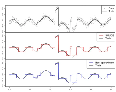
Fig 4. Performance of SMUCEfˆnwith thresholdη(0.1)as oracle approximants for the signal
in Olshen et al. (2004) and Zhang and Siegmund (2007). The bottom panel shows the best approximant fappˆ
Kn, defined in (14), of the truth with up to
ˆ
Kn jumps. Here SNR= 3 and f−fˆnL2= 1.3f−fappˆ KnL 2. ≥Pfn−fKappˆnL2 ≥C5fn−fˆnL2 ≥P{An} →1 as n→ ∞, which concludes the proof.
Remark 10. Proposition2indicates that ˆfnperforms almost (up to a constant) as well as the best approximants fappˆ
Kn for “complicated” functions f0 in A
γ
2,L, see Figure 4 for a visual illustration. For simpler functions f0 in Aγ2,L, e.g.,
f0 is piecewise constant, note that f0 −fKappˆ nL
2 can be zero. Thus, in this sense, the result in Proposition 2 cannot be improved by replacing supf0∈Aγ
2,L
by inff0∈Aγ
2,L.
6. Simulation study
Note that in the optimization problem (4) for MCPS methods, we optimize only over the local intervals, where the candidate function is constant, cf. (5). This leads to independence of values of candidate function among different segments, and thus ensures the structure of (4) to be a directed acyclic graph, which makes
3275
dynamic programmingalgorithms (cf. Bellman,1957) applicable to such a prob-lem, see also Korte and Vygen (2012, Chapter 7). Moreover, the computation can be substantially accelerated by incorporating pruning ideas as e.g. recently developed in Killick, Fearnhead and Eckley (2012), Frick, Munk and Sieling (2014) and Li, Munk and Sieling (2016). As a consequence, the computational complexity of MCPS methods can be even linear in terms of the number of observations, in case that there are many change-points, see Frick, Munk and Sieling (2014) and Li, Munk and Sieling (2016) for further details.
We now investigate the finite sample performance of MCPS methods from the previously discussed perspectives. For brevity, we only consider a particular MCPS method, SMUCE (Frick, Munk and Sieling, 2014), and stress that the results are similar for other methods of type (4) (which are not shown here), see e.g. Frick, Munk and Sieling (2014) and Li, Munk and Sieling (2016) for an extensive simulation study. For SMUCE, we use the implementation of a pruned dynamic program from the CRAN R-package “stepR”, select the system of all intervals with dyadic lengths for the multiscale constraint, and chooseη=η(β) in (7) as the threshold, which is estimated by 10,000 Monte-Carlo simulations. In what follows, the noise is assumed to be Gaussian with a known noise level
σ, and SNR denotes the signal-to-noise ratio fL2/σ.
6.1. Stability
We first examine the stability of MCPS methods with respect to the significance level β, i.e. to the threshold η. The test signalf0 (adopted from Olshen et al., 2004; Zhang and Siegmund,2007) has 6 change points at 138, 225, 242, 299, 308, 332, and its values on each segment are −0.18, 0.08, 1.07, −0.53, 0.16, −0.69,
−0.16, respectively. Figure 5 presents the behavior of SMUCE with threshold
η =η(β) for different choices of significance levelβ, on some specific data (see Table 1 in Frick, Munk and Sieling (2014) for the performance over many random repetitions). In fact, for the shown data, SMUCE detects the correct number of change-points, and recovers the location and the height of each segment in high accuracy, for the whole range of 0.06≤ β ≤0.94 (i.e. 0.47√logn≥ η ≥
−0.04√logn). Only for smallerβ (<0.06, i.e.η >0.47√logn), SMUCE tends to underestimate the number of change-points (see the second panel of Figure5
for example, where the missing change-point is marked by a vertical solid line), while, for largerβ (>0.94, i.e.η <−0.04√logn), it is inclined to recover false change points (as shown in the last panel of Figure 5). Note that in either case the estimated locations and heights of the remaining segments (away from the missing/spurious jumps) are fairly accurate. This reveals that SMUCE is remarkably stable with respect to the choice of β (or η), in accordance with Theorem1, Remark3 and Proposition1.
6.2. Different noise levels
We next investigate the impact of the noise level (or equivalently SNR) on MCPS methods. We consider the recovery of the Blocks signal (Donoho and
3276
Fig 5. Estimation of the step signal in Olshen et al. (2004) and Zhang and Siegmund (2007)
by SMUCE withη=η(β)for differentβ(sample sizen= 497, and SNR= 1).
Johnstone,1994) for different noise levels. The result for SMUCE at significance level β = 0.1 is summarized in Figure 6 and Table 1. It shows that SMUCE recovers the truth rather well, in terms of e.g. change-point locations and L2
-loss, for the low and medium noise levels (SNR = 2.5 or 2), while it tends to miss one or two small scale features for the high noise level (SNR = 1.5).
6.3. Robustness and feature detection
In order to investigate the robustness of MCPS methods with respect to model misspecification, we introduce a local trend component as in Olshen et al. (2004) and Zhang and Siegmund (2007) to the test signalf0in Section6.1, which leads
to the model (withn= 497)
yin=f¯in+ 0.25bsin(aπi)+ξin, i= 0, . . . , n−1. (15) We consider two scenarios separately.
(i) Weak background waves. We simulate data for a = 0.025 and b = 0.3, and apply SMUCE again with various choice of β, see Figure 7, with
3277
Fig 6. Blocks signal: SMUCE for various noise levels (sample sizen=1,023).
the average performance given in the top part of Table2. It shows that SMUCE captures all relevant features, e.g., change-points and modes, of the piecewise constant part (cf. Figure7) of the true signal, and is stable with respect to the choice of β. This is in accordance with the previous simulations and Theorems3 and5.
(ii) Strong background waves.When the scale b of the background wave be-comes larger, i.e., the fluctuation is stronger, SMUCE captures the fluctu-ation by including additional change-points according to Theorems2,3,5
and Proposition2. Figure8, as well as Table2, illustrates the performance of SMUCE withβ = 0.1 for the signal in (15) with b = 1.0 and b = 1.2
Table 1
Performance of SMUCE (β= 0.1) on the Blocks signal (n= 1,023, cf. Figure6) for various noise levels over 100 random repetitions.
SNR Counts of #J( ˆfn)−#J(f0) Average of
≤ −2 −1 0 ≥1 n·d(J( ˆfn), J(f0)) fˆn−f0L2/f0L2
2.5 0 1 99 0 1 0.046
2 0 16 84 0 4.2 0.071
3278
Fig 7. Estimation of the signal in (15)(a= 0.025, b= 0.3) by SMUCE with η=η(β) for
differentβ(SNR= 1).
under different noise levels. It can be seen that SMUCE recovers the shape and modes of the whole true signal (which has 8 modes in total).
We stress, moreover, that by Theorem4it is possible to screen whether the recovered features are genuine or not with pre-specified confidence levelβ. This can be done by the procedure detailed in Remark8. From Table2, we observe that nearly all the recovered features are genuine when the noise level is low (e.g., SNR = 2.5), while only large features are guaranteed to be there for the medium and high noise levels (e.g., SNR = 2 or 1.5), with probability at least 90%. This is mainly due to the built-in parsimony of the method, namely, the minimization of number of change-points, see (4).
6.4. Empirical convergence rates
Finally, we empirically explore how well the finite sample risk is approximated by our asymptotic analysis. The test signals are the Blocks and the Heavisine from Donoho and Johnstone (1994). Note that the Blocks signal is a piecewise constant function with a fixed number of change-points, so the convergence rates
3279
Fig 8. Estimation of the signal in (15) with a= 0.025 and b = 1 or 1.2 by SMUCE for
various noise levels.
Table 2
Average performance of SMUCE (β= 0.1) on the signal in (15)(a= 0.025, cf. Figures7
and8) over 100 random repetitions. The number of inferred modes is computed according to the procedure in Remark8.
b SNR #J( ˆfn)−#J(f0) #mode( ˆfn) # inferred modes fˆn−f0L2/f0L2
0.3 2.5 0.51 2.2 2.1 0.17 2 0.14 2 2 0.17 1.5 −0.09 1.9 1.5 0.21 1 2.5 9.1 6 5.5 0.27 2 8.5 5.8 3.7 0.31 1.5 4.8 3.5 1.7 0.45 1.2 2.5 9.2 6 5.8 0.3 2 8.9 5.9 4.9 0.32 1.5 6.3 4.4 2.1 0.45
inL2-risk is of ordern−1/2(up to a log-factor) by Theorem1. For the Heavisine
signal, the convergence rate is of order n−1/3 (up to a log-factor), since it lies
in H1
1,L and BVL for some L, see Theorem 2 and Example 1. Although the Heavisine also lies in Hα
1,L, α ≥ 1, this will not lead to a faster rate for the MCPS methods due to the saturation phenomenon, see Example2.