Available at:
http://hdl.handle.net/2078.1/152766
"A simple model for now-casting volatility series"
Breitung, Jorg ; Hafner, ChristianAbstract
Nowcasting volatility of financial time series appears difficult with classical volatility models. This paper proposes a simple model, based on an ARMA representation of the log-transformed squared returns, that allows to estimate current volatility, given past and current returns, in a very simple way. The model can be viewed as a degenerate case of the stochastic volatility model with perfect correlation between the two error terms. It is shown that the volatility nowcasts do not depend on this correlation, so that both models provide the same nowcasts for given parameter values. A simulation study suggests that the ARMA and SV models have a similar performance, but that in cases of moderate persistence the ARMA model is preferable. An extension of the ARMA model is proposed that takes into account the so-called leverage effect. Finally, the alternative models are applied to a long series of daily S&P 500 returns.
Document type : Document de travail (Working Paper)
Référence bibliographique
Breitung, Jorg ; Hafner, Christian. A simple model for now-casting volatility series. CORE Discussion Papers ; 2014/60 (2014) 19 pages
2014/60
■A simple model for now-casting volatility series
Jörg Breitung and Christian M. Hafner
Center for Operations Research
and Econometrics
Voie du Roman Pays, 34
B-1348 Louvain-la-Neuve
Belgium
http://www.uclouvain.be/core
D I S C U S S I O N P A P E R
CORE
Voie du Roman Pays 34, L1.03.01 B-1348 Louvain-la-Neuve, Belgium. Tel (32 10) 47 43 04
Fax (32 10) 47 43 01
CORE DISCUSSION PAPER 2014/60
A simple model for now-casting volatility series
J¨org Bereitung1 and Christian M. Hafner⇤2 1University of Cologne
2Universit´e catholique de Louvain
November 19, 2014
Abstract
Nowcasting volatility of financial time series appears difficult with classical volatility models. This paper proposes a simple model, based on an ARMA representation of the log-transformed squared returns, that allows to estimate current volatility, given past and current returns, in a very simple way. The model can be viewed as a degenerate case of the stochastic volatility model with perfect correlation between the two error terms. It is shown that the volatility nowcasts do not depend on this correlation, so that both models pro-vide the same nowcasts for given parameter values. A simulation study suggests that the ARMA and SV models have a similar performance, but that in cases of moderate persistence the ARMA model is prefer- able. An extension of the ARMA model is proposed that takes into account the so-called leverage e↵ect. Finally, the alternative models are applied to a long series of daily S&P 500 returns.
Keywords: EGARCH, stochastic volatility, ARMA, realized volatility, leverage
JEL Classification: C22, C58
⇤ Corresponding author, Institute of statistics, biostatistics and actuarial
sci-ences, and CORE, Universit´e catholique de Louvain, Voie du Roman Pays 20, 1348 Louvain-la-Neuve, Belgium, email: [email protected].
The authors would like to thank seminar participants at Humboldt-University Berlin, University of Cologne, University of Salerno, University of St Andrews, University of Cambridge, Tinbergen Institute Amsterdam, and in particular Gi-ampiero Gallo, Siem Jan Koopman and Roman Liesenfeld, for helpful comments and discussions.
A simple model for now-casting volatility series
J¨org Breitung
1and Christian M. Hafner
∗21
University of Cologne
2
Universit´
e catholique de Louvain
November 19, 2014
Abstract
Nowcasting volatility of financial time series appears difficult with classical volatility models. This paper proposes a simple model, based on an ARMA representation of the log-transformed squared returns, that allows to estimate current volatility, given past and current returns, in a very simple way. The model can be viewed as a degenerate case of the stochastic volatility model with perfect correlation between the two error terms. It is shown that the volatility nowcasts do not depend on this correlation, so that both models provide the same nowcasts for given parameter values. A simulation study suggests that the ARMA and SV models have a similar performance, but that in cases of moderate persistence the ARMA model is prefer-able. An extension of the ARMA model is proposed that takes into account the so-called leverage effect. Finally, the alternative models are applied to a long series of daily S&P 500 returns.
Some key words: EGARCH, stochastic volatility, ARMA, realized volatility, leverage
JEL Classification Number: C22, C58
∗Corresponding author, Institute of statistics, biostatistics and actuarial sciences, and CORE,
Uni-versit´e catholique de Louvain, Voie du Roman Pays 20, 1348 Louvain-la-Neuve, Belgium, email:
The authors would like to thank seminar participants at Humboldt-University Berlin, University of Cologne, University of Salerno, University of St Andrews, University of Cambridge, Tinbergen Insti-tute Amsterdam, and in particular Giampiero Gallo, Siem Jan Koopman and Roman Liesenfeld, for helpful comments and discussions.
1
Introduction
The literature on volatility models continues to grow steadily, driven mainly by the suc-cess that these models encounter in modelling financial time series, but also by the non-exhausted understanding of some of their properties and their estimators. The main benchmark remains the classical GARCH model, introduced by Engle (1982) and Boller-slev (1986), due to its simplicity in estimation and widespread availability in software packages. The GARCH model is essentially a model for predicting volatility for today, given past observations. It does so quite well, as demonstrated by Andersen and Bollerslev (1998) by using a realized volatility target instead of the commonly used daily squared returns. However, the GARCH model does not offer the possibility to update a prediction with today’s observed data. In other words, nowcasting volatility in the GARCH model corresponds to using predicted volatility, ignoring today’s observation.
Consider the ordinary GARCH(1,1) specification for the volatility process ˜ht
yt= q ˜ htξt (1) ˜ ht=yb2t|t−1 ≡ E(y 2 t|y 2 t−1, y 2 t−2, . . .) (2) =µ+αy2 t−1+φ˜ht−1 (3)
where ξt is i.i.d. with E(ξt) = 0 and E(ξt2) = 1. Lettingy 2
t = ˜ht+vt we can replace ˜ht by
y2
t −vt yielding the ARMA representation of y2t:
y2
t =µ+ (α+φ)y 2
t−1+vt−φvt−1. (4)
Accordingly, the volatility process is equivalent to the linear forecast of y2
t conditional on
{yt−1, yt−2, . . .} and the variance process results from a filtration of the form
˜ ht= µ 1−φ +α ∞ X i=1 φiy2 t−i. (5)
An important drawback of the standard GARCH model is that the observation y2 t does
not enter the variance process, which is arguably the most important information about current volatility. This pitfall has been noted, for instance, by Politis (2007) among others. In this paper we propose a simple variant of the (exponential) GARCH model that exploits the information in the current observationyt. Assumingεt= logξt2
iid
∼ N(µ, σ2
ε) the model
parameters can be estimated efficiently by fitting an ARMA(1,1) model to the transformed series xt = logyt2. In contrast to the GARCH(1,1) the log variance process in our model
results from the filtration E(log ˜ht|xt, xt−1, . . .) =c+ 1− θ β X∞ i=0 θixt−i , (6)
where θ and β are typically positive parameters, close to unity with θ < β and c is a constant.
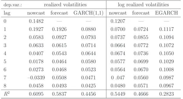
To appreciate the importance of the current observation for estimating (“nowcasting”) volatilities we computed realized volatilities as the quadratic variation of the squared returns from 5-minute intervals of the S&P 500 index obtained from the Oxford Man Institute Realized Library. To investigate how well these volatilities (Vt) can be estimated
by fitting a linear filter of the daily returns (rt−i, the log differences of the opening and
closing price) we fit a distributed lag model of the form Vt=µ+ 8 X i=0 βir2t−i+et (7) or logVt=β0+ 8 X i=0 βilogr 2 t−i +e∗t. (8)
It should be noted that the realized volatilities are computed as Vt =Pnj=1r 2
j,t, whereas
the squared daily return result as r2 t =
Pn j=1rj,t
2
, where rj,t denotes the 5-minute
intraday return. The n(n− 1) cross-terms rj,trk,t with j 6= k give rise to a very noisy
estimator of daily variances and, thus, some smoothing is required to obtain reliable results. Table 1 presents the estimates for β0, . . . , β8. It turns out that the current
observation contributes substantially to the variance process in particular for the log realized volatility series. The GARCH(1,1) and the EGARCH model provide a reasonable but less accurate approximation to the weight function.
2
The nowcasting model
To exploit the information in the current observation yt we consider the following model
for a series of financial returns yt,
yt = exp(ht/2)ξt, ξt ∼i.i.d.(0,1) (9)
ht = α+βht−1+κεt , (10)
where εt = log(ξt2)− C ∼ i.i.d.(0, σ 2
ε) and C = E[log(ξ 2
t)]. Log volatility ht in (10)
independent of ξt, the error term εt in (10) is an explicit function of the innovation term
ξt in (9). Some more comparisons with the stochastic volatility model will be given in
Section 4.
Let us first discuss some properties of model (9)-(10). If the distribution of ξt is
known, then the parameter C is identified. For example, for Gaussian ξt, C ≈ −1.27.
In what follows we assume that C is unknown and absorb E[log(ξ2
t)] into the constant
α. At the end of Section 3 we discuss how to estimate this constant. Note also that mean and variance of log volatility are given by, respectively, E[ht] = α/(1−β) and
Var(ht) =κ2σε2/(1−β 2
), and σ2
ε depends on the distribution ofξt. Ifξt is Gaussian, then
σ2 ε =π
2
/2.
Under the assumption that ξt has a symmetric distribution it follows thatyt is a
mar-tingale difference series, i.e. Et−1[yt] = 0, where Et−1[·] denotes expectation conditional
on{yt−1, yt−2, . . .}. This results from
Et−1[yt] =Et−1[exp{(α+βht−1)/2}]E[exp(κ/2 logξt2)ξt],
where the second expectation on the right hand side is zero since it is the expectation of an odd function of ξt. Thus, as in classical ARCH or stochastic volatility models, the
return series yt has a conditional mean of zero, and all temporal dependence is captured
via the log volatility process ht.
We now transform model (9) – (10) to obtain a linear process for the transformed variable. Defining xt= logyt2, we have
xt =ht+εt (11)
and, replacing ht−1 in (10) by xt−1−εt−1,
ht = α+βxt−1+κεt−βεt−1 (12)
xt = α+βxt−1+ (1 +κ)εt−βεt−1 . (13)
Indeed, the transformed returns xt in (13) follow an ARMA(1,1) process.
It is interesting to compare this model specification with two popular GARCH alterna-tives: First, the (symmetric version of the) EGARCH model suggested by Nelson (1991) replaces (10) by the equation
ht=α+βht−1 +ψ|ξt−1|. (14)
Here, log-volatilities are driven by lagged values ξt−1 instead of the current values ξt.
shocks ξthave a much stronger effect in model (14). The proposed model (10) is actually
closer to the so-called log-GARCH model, introduced independently by Geweke (1986) and Pantula (1986), where xt is as in (11) with ht given by
ht=α+βht−1+ψlogy 2
t−1 (15)
which leads to the ARMA representation
xt=α+ (ψ+β)xt−1+εt−βεt−1. (16)
Notice the difference with respect to the ARMA representation (13), in which the coeffi-cient κcaptures the impact of the current observation on volatility in the moving average part, which is shifted to a lagged effect ψxt−1 in the autoregressive part of (16).
3
The reduced form ARMA representation
An observationally equivalent ARMA(1,1) model for xt is obtained from
xt =α+βxt−1+ (1 +κ)εt−
β
1 +κ(1 +κ)εt−1
=α+βxt−1+ut−θut−1 , (17)
where ut = (1 +κ)εt is white noise with variance σu2 = (1 +κ) 2
σ2
ε and θ = β/(1 +κ).
The relationship between the reduced form parameters θ, σ2
u =E(u 2
t), and the structural
parameters κ, σ2 ε is given by κ = β/θ−1 (18) σ2 ε = θ β 2 σ2 u. (19)
Since εt = ut/(1 +κ) = (θ/β)ut, the variance component ht can be estimated from the
reduced form as
bht=xt−
θ
βut. (20)
Note that (20) is measurable w.r.t. present and past values ofxt, because the reduced form
is invertible and we have ut=−α/(1−θ) +φ(L)xt withφ(L) = (1−θL)−1(1−βL). By
comparing coefficients of the lag polynomials, one obtainsφ(L) = 1+(1−β/θ)P∞j=1θjLj.
Inserting this result into (20), we obtain
bht= θα β(1−θ)+ 1− θ β X∞ j=0 θjxt−j. (21)
This shows that the filtered volatility is a linear combination of present and past values of xt with exponentially declining weights.
(Pseudo) ML estimators of the structural parameters (β, κ, σ2
ε) are obtained by
insert-ing the ML estimators of the reduced form (β, θ, σ2
u) into (18) and (19). Based on the
consistency and asymptotic normality of the reduced form maximum likelihood estima-tors, we can find similar results for the estimators of the structural form using the delta method. This gives closed form expressions for the asymptotic variances of√n( ˆβ−β) and √
n(ˆκ−κ), see Appendix A.1. Note that in practice,θ is often close to unity. Therefore, an exact ML estimation method rather than a conditional ML estimator (treating the start-ing value as fixed) should be employed. Whenever εt = log(ξt2) is normally distributed,
then the ML estimator is asymptotically efficient.
Estimation of the constant. The ARMA approach yields an estimator forh∗t =C+ht
and therefore an estimator for C is required to estimate ht. From (11) it follows that
y2 t =eh ∗ t−Cξ2 t = c eh ∗ tξ2 t ,
where c= exp(−C) and
ξ2 t = y2 t c eh∗ t .
Since we assume that E(ξ2
t) = 1 we can estimate the constant from the estimated values
of ξ2 t as 1 T T X t=1 b ξ2 t = 1 ⇔ bc = 1 T T X t=1 y2 t ebh∗ t , wherebh∗
t =xt−(bθ/βb)but denotes the ARMA estimator of the volatility series.
4
Relationship to the stochastic volatility model
It is interesting to compare our approach to the stochastic volatility (SV) model, where (10) is replaced by
assuming thatξt and ηt are independent. The ARMA representation results as
xt =α∗+βxt−1+ηt+εt−βεt−1 . (23)
whereεt= log(ξt2)−C. Again we can find a second-order equivalent reduced form ARMA
model as in (17), i.e.
xt =α∗+βxt−1+ut−θut−1 , (24)
that is, the autocovariance functions of xt in (23) and (24) are identical. Accordingly, the
model parameters of the SV model can be seen as transformations of the reduced form parameters in (24). Specifically we have
σ2 u(1 +θ 2 ) =σ2 η +σ 2 ε(1 +β 2 ) (25) θσ2 u =βσ 2 ε. (26) It follows that σ2 ε = θ βσ 2 u (27) σ2 η = 1− θ β −θ(β−θ) σ2 u . (28)
The Kalman filter applied to the state space representation of this model delivers the filtered volatility
ht|t= (1−θ/β)xt+ (θ/β)ht|t−1
where the predicted volatility ht|t−1 is given by
ht|t−1 =α+ (β−θ)xt−1 +θht−1|t−2 Hence, we obtain ht|t = θ β α 1−θ + κ 1 +κ ∞ X j=0 θjxt−j = θα β(1−θ) + 1− θ β X∞ j=0 θjxt−j
which shows that the SV filtered volatility is equivalent to the filtered volatility using the ARMA model given by (21).
In the next proposition we show that this result extends to the class of models with an arbitrary error correlation:
Proposition 1 Let xt = ht +εt, where ht = α +βht−1 + ηt, ηt ∼ i.i.d.(0, σ2η), εt ∼
i.i.d.(0, σ2
ε) and arbitrary covariance E(ηtεt) = ρσεση with ρ∈[−1,1]. It follows that
ht|t = θα β(1−θ) + 1− θ β X∞ j=0 θjxt−j
The proof is provided in Appendix A.2.
Our model in (10) corresponds to the case ρ = 1, while the classical SV model (22) results from setting ρ = 0. It follows from Proposition 1 that for the estimation of ht
based on the information setxt, xt−1, . . .the correlation betweenεtandηtdoes not matter.
Therefore, there is no need to invoke Kalman filter recursions to estimate the variance process.
Note that a non-zero correlation between εt and ηt does not imply that ξt and ηt are
correlated. The latter case attracted some interest to model the so-called leverage effect in stochastic volatility, see e.g. Harvey and Shephard (1996). For example, consider our model (9)-(10), i.e. the degenerate case of Proposition 1 withρ= 1,ηt=κεt, and suppose
that the distribution of ξt is symmetric. Then, the correlation between ξt and ηt is zero
even though εt and ηt are perfectly correlated. To include a leverage effect, the model
needs to be extended, which we will do in Section 6.
Note also that, according to Harvey and Koopman (2000), the model (22) with cor-relatedεt andηt is said to be in the contemporaneous state form. If one replaces (22) by
ht+1 =α+βht+ηt with correlated εt and ηt, then the model is said to be in the future
state form. As Harvey and Koopman (2000) show for the case of a random walk plus noise (i.e. β = 1), the filtered estimator of ht depends onρin the future state model, but
not in the contemporaneous state model.
Finally, if the distribution ofξtis symmetric, then it can be shown that the white noise
ut of the reduced form ARMA representation (24) is serially uncorrelated. In general,
however, it is not a martingale difference, as e.g. E[utx2
t−1] 6= 0, see Francq and Zakoian
(2006). The fact that ut in the ARMA representation of the SV model is neither i.i.d.
nor a martingale difference also has implications for inference. The general sandwich type formula for the asymptotic covariance matrix of QMLE estimators remains valid, but it is not available in closed form and it is different from the asymptotic covariance matrix of our model, given in Appendix A.1. Thus, although for given parameters both models yield the same filtered volatility estimates, estimation and inference are different due to the different properties of the error term ut.
5
Finite sample properties
In this section we compare the finite sample properties of alternative estimators for volatil-ities. The data are generated as
yt=eht/2ξt t = 1, . . . , T ,
where ht is either
ARMA: ht =α+βht−1+κεt (29)
or SV : ht =α+βht−1+ηt . (30)
The error process εt = log(ξt2) + 1.27 with ξt iid
∼ N(0,1) is independent of ηt iid
∼ N(0, σ2 η).
Accordingly, in the stochastic volatility model (SV) xt= logy2t is composed of two
inde-pendent processes, whereas in the ARMA modelxtis driven by a single stochastic process
εt.
First, consider the case where the generated volatility is a classical stochastic volatility process. We follow Sandmann and Koopman (1998) in specifying the parameters of the SV model. Defining the coefficient of variation, CV = Var[exp(ht)]/E[exp(ht)]2, one
obtains the expression CV = exp(σ2
η/(1−β 2
))−1. The coefficient of variation for this model is directly related to the kurtosis of yt, which is given by κ = 3(CV + 1). Here,
α is an irrelevant scaling parameter, but Sandmann and Koopman (1998) determine
α such that E[ht] = 0.0009, which gives a realistic annualized standard deviation of
22%. To distinguish between highly and moderately persistent volatility processes, we fix β alternatively at 0.98 and 0.90. Similarly, to evaluate the effects of high versus low coefficients of variation (or, equivalently, high versus low kurtosis), we fixCV alternatively at 10 and 1, with corresponding kurtosis coefficients 33 and 6, respectively. This gives four different parameterizations. The sample sizes are T = 500 and 2000. Each process is simulated k = 1000 times.
The volatilities of the processytare estimated by fitting a symmetric EGARCH model,
a symmetric SV model, and the ARMA approach proposed in Section 3, where the con-stant is estimated as suggested in Section 3. The performance is measured by an R2
criterion computed as e R2 h = 1− T P t=1 (ht−bht)2 T P t=1 (ht−¯h)2 where ¯h = T−1PT
t=1ht. This variant of the usual R 2
imposes a zero constant and a unit scaling coefficient in order to measure the correspondence of the estimates with the original volatility process. Table 2 reports the results.
Not surprisingly, the R2
measures of the EGARCH fit are substantially smaller in all cases, due to the smaller information set that is used in estimation. Also not surprisingly, the R2
of SV and ARMA are close to each other, since both models deliver the same filtered volatility estimate for given parameters. Hence, the differences between them are solely due to differences in parameter estimates. Note that the ARMA R2
tends to be higher when the persistence is moderate (β = 0.9). Note also that for increasing sample size, theR2
does not need to improve, because the sample size affects the estimation error but not the signal to noise ratio determined essentially by σ2
η and σ 2 ε.
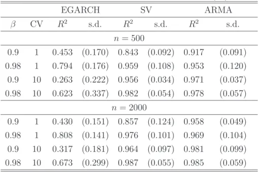
In the second simulation setup we generate reduced form ARMA processes for htwith
parameters chosen analogously to the SV case. More precisely, the persistence parameter
β and the intercept α are the same as in SV. The moving average parameter θ is chosen such that CV ∈ {1,10}, as before, by expressingθ as a function ofση,β, andσε. Results
are reported in Table 3. Overall, the R2
tends to be higher than in the SV case, which is plausible as there is no second noise term in the volatility equation. Furthermore, volatility is a measurable function of today’s and lagged information. Thus, for increasing sample size we expect the R2
to converge to unity, which happens for both estimation methods based on ARMA and SV. Again we observe the same effect as for a true SV process where the ARMA R2
is higher for moderate persistence.
6
An asymmetric extension
In order to account for the leverage effect that is often encountered in empirical applica-tions, we define the dummy variable dt =I(yt > τ), where I(·) is the indicator function,
and τ is a predefined threshold (which is typically zero), the mean of yt, or some other
An asymmetric extension of the above model is given by
ht=α+βxt−1+κ +
dtεt+κ−(1−dt)εt−βεt−1, (31)
which we call ARMA model with leverage, or ARMA-L. Note that in contrast to Nelson’s EGARCH model and other asymmetric GARCH models, the asymmetric effect in this model is contemporaneous and not lagged.
The structural form for xt results as
xt=α+βxt−1+ (1 +κ +
)dtεt+ (1 +κ−)(1−dt)εt−βεt−1. (32)
Denote again the MA part of this model byvt = (1 +κ+)dtεt+ (1 +κ−)(1−dt)εt−βεt−1.
We have the following conditional second order moment structure.
Var(vt|dt) = ((1 +κ+)2dt+ (1 +κ−)2(1−dt) +β2)σ2εt (33)
E[vtvt−1|dt] = −{(1 +κ+)dt+ (1 +κ−)(1−dt)}βσ2
εt (34)
We can find an observationally equivalent ARMA(1,1) process
xt=α+βxt−1+ut−θ+dtut−1−θ−(1−dt)ut−1. (35)
This process has the same conditional second order moment structure provided that
κ+ = β/θ+ −1 (36) κ− = β/θ−−1 (37) σ2 εt = {(1 +κ + )2 dt+ (1 +κ−)2(1−dt)}−1σu2 (38)
Note that the error termεtis conditionally heteroskedastic. If the estimated model (35) is
invertible, then it is easy to check that the model (32) with parameters given by (36)-(38) will also be invertible.
We could have chosen the alternative solution
κ+ = βθ+ −1 (39) κ− = βθ−−1 (40) σ2 ε = σ2 u β2 (41)
which is conditionally homoskedastic. However, if the estimated model (35) is invertible, then the model (32) with parameters given by (39)-(41) will not be invertible, and is therefore excluded.
Note that the process (35) is similar to the asymmetric ARMA model proposed by Br¨ann¨as and De Gooijer (1994), the difference being that in their model, the indicator variable is specified as dt = I(ut−1 > 0). The model (35) can be estimated by quasi
maximum likelihood. To obtain the information matrix, the Hessian can be approximated by the sum of the outer products of the gradient as in Br¨ann¨as and De Gooijer (1994).
7
An empirical application
We apply our model on a large dataset, the demeaned daily (close to close) return on the S&P 500 index from 1/1/1950 — 25/10/2012, a total of 16,058 observations. We first estimate the classical EGARCH(1,1) with N(0,1) innovations, as proposed by Nelson (1991):
yt = exp(ht/2)ξt, ξt∼N(0,1)
ht = α+βht−1−θξt−1+γ|ξt−1|
This model is estimated by maximum likelihood, and the results are shown in Table 4. We estimate the SV model (22) by QMLE and the Kalman filter, assuming ηt ∼
N(0, σ2
η) and εt ∼ N(0, σε2). Results are also presented in Table 4. The estimators of σ 2 η
and σ2
ε correspond to (28) and (27).
The ARMA(1,1) model in (17) is estimated using nonlinear least squares with numeri-cal optimization. For the nonlinear ARMA model with leverage (ARMA-L), see equation (31), we choose a threshold τ =−0.01, corresponding to one negative unconditional stan-dard deviation of returns yt. Estimation results for the three models are also reported
in Table 4. All three models pass portmanteau specification tests applied to the squared residuals ˆξ2
t.
The persistence of shocks to volatility measured by β is even higher in the ARMA models than for EGARCH. The parameter estimate of κ implied by the estimates of θ
andβ is given by ˆκ = ˆβ/θˆ−1 = 0.0391 for the ARMA model, and ˆκ+ = ˆβθˆ+−1 = 0.0353
and ˆκ− = ˆβθˆ− −1 = 0.0605 for the ARMA-L model. The estimated volatility process
ˆ
h∗
t is adjusted by the estimated constant ˆC = −log(ˆc), where ˆc is the sample mean of
y2
t/exp(ˆh∗t), see Section 3. Table 4 also presents the sample variances of the error terms
εt =xt−ht, which are clearly smaller for the ARMA models, as expected.
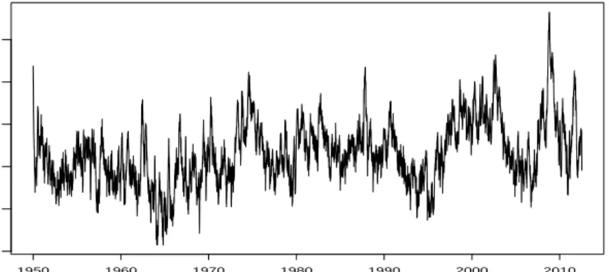
Figure 1 shows the nowcast of log volatility using the ARMA-L model (31), and the predicted log-volatility of the EGARCH model. The sample correlation between both
volatility series is 91%. The predicted EGARCH volatility was higher after the October 1987 crash than after the Lehman crisis 2008, while the updated ARMA volatility was higher for the Lehman crisis. An explanation might be that the 1987 crash was mainly driven by an exceptionally severe one-day drop of returns, while absolute returns were exceptionally high during a longer time period around the Lehman crisis.
8
Conclusions
The proposed ARMA representation of log squared returns provides a simple method for estimating current volatility given the past and current information on the underlying returns. Our results suggest that it outperforms predictions of GARCH-type models, and similarly to stochastic volatility models while being easier to estimate.
We have proposed an important extension of the model to incorporate the so-called leverage effect. Many other extensions are possible and indeed object of future work. For example, it is straightforward to include a ”GARCH-in-mean”-type risk premium in the conditional mean of returns, where the risk premium would depend on the current volatility, not on the predicted one. Second, multivariate extensions are possible. For example, one could use a factorization as in the orthogonal GARCH model of Alexander (2001). We believe that these are important topics of future research.
Appendix
A.1 Asymptotic distribution of estimators
Under our conditions, the maximum likelihood estimator ˆγ = ( ˆβ,θˆ) of the reduced form ARMA model (17) is consistent and asymptotically normal with asymptotic distribution given by √ n(ˆγ−γ)→dN 0, 1−βθ (β−θ)2 " (1−β2 )(1−βθ) −(1−θ2 )(1−β2 ) −(1−θ2 )(1−β2 ) (1−θ2 )(1−βθ), #!
see e.g. Brockwell and Davis (1991). This gives directly the asymptotic variance of √
n( ˆβ −β), while that of √n(ˆκ−κ) is obtained via the delta method. Straightforward calculations yield nVar(ˆκ)→ (1−βθ) 2 (β−θ)2 1−θ2 θ2 (1−β 2 ) 1 1−θ2 + 2β θ(1−θβ)+ β2 θ2(1 −β2) .
A.2 Proof of Proposition 1
Denote Xt = σ(xt, xt−1, xt−2, . . .) and let ht|t−1 = E[ht|Xt−1], ht|t = E[ht|Xt], and Vt =
Var(ht|Xt−1). First we note that
ut=xt−E(xt|Xt−1) =ht−ht|t−1+εt
=α+ηt+β(ht−1−ht−1|t−1) +εt .
The estimator of the log-variance process is
ht|t=ht|t−1+ V
t+E[(ht−ht|t−1)εt]
Vt+ 2E[(ht−ht|t−1)εt] +σε2
ut (42)
where E[(ht−ht|t−1)εt] = E(ηtεt), which follows from the Kalman filter with correlated
measurement and transition errors, see e.g. Section 3.2.4 of Harvey (1989). For the case of correlated errors, equation (26) generalizes to
Var(ut) =Vt+σε2+ 2E(ηtεt)
= β
θ[σ
2
ε +E(ηtεt)]
which is the denominator in the second term of the right hand side of (42). The numerator is obtained by subtracting from this expression σ2
ε +E(ηtεt), and we obtain Vt+E(ηtεt) = β θ −1 [σ2 ε+E(ηtεt)] =κ[σ2 ε +E(ηtεt)]
We finally obtain ht|t=ht|t−1+ V t+E(ηtεt) [Vt+E(ηtεt)] + [σε2+E(ηtεt)] ut =ht|t−1+ κ 1 +κut .
Since ht|t−1 is identical to the forecast of xt based on the xt−1, xt−2, . . ., the estimator ht|t
is invariant to the covarianceE(ηtεt). Therefore, ht is identical to the estimator based on
perfect correlation with εt=κηt which is given in (21). ✷
References
Alexander, C.O. (2001), Orthogonal GARCH, in Mastering Risk, Volume II, edited by C.O. Alexander, pp. 21–38, Prentice Hall.
Andersen, T. and Bollerslev, T. (1998), Answering the skeptics: Yes, standard volatility models do provide accurate forecasts, International Economic Review, 39, 885-905.
Bollerslev, T.(1986), Generalized autoregressive conditional heteroskedasticity, Jour-nal of Econometrics, 31, 307-327.
Br¨ann¨as, K. and De Gooijer, J.G. (1994), Autoregressive-asymmetric moving av-erage models for business cycle data,Journal of Forecasting 13, 529-544.
Engle, R.F.(1982), Autoregressive conditional heteroscedasticity with estimates of the variance of United Kingdom inflation, Econometrica, 50, 987-1007.
Francq, C. and Zakoian, J.-M. (2006), Linear-representation based estimation of stochastic volatility models, Scandinavian Journal of Statistics 33, 785-806.
Geweke, J. (1986). Modelling the Persistence of Conditional Variance: A Comment.
Econometric Reviews5, 5761.
Harvey, A. (1989), Forecasting, structural time series models and the Kalman filter, Cambridge University Press.
Harvey, A. and Koopman, S.J. (2000), Signal extraction and the formulation of unobserved components models, Econometrics Journal 3, 84-107.
Harvey, A. and Shephard, N. (1996), Estimation of an asymmetric stochastic volatility model for asset returns, Journal of Business & Economic Statistics 14, 429-434.
Nelson, D. (1991), Conditional heteoskedasticity in asset returns: A new approach.
Econometrica 59, 347-370.
Pantula, S. (1986). Modelling the Persistence of Conditional Variance: A Comment. Econometric Reviews 5, 7173.
Politis, D.N. (2007), Model-free versus Model-based Volatility prediction, Journal of Financial Econometrics 5, 358–359.
Sandmann, G. and Koopman, S.J.(1998). Estimation of stochastic volatility models via Monte Carlo maximum likelihood. Journal of Econometrics, 87, 271-301.
S&P500 ARMA log v ar iance 1950 1960 1970 1980 1990 2000 2010 −12 −11 −10 −9 −8 −7
(a) Nowcast log volatility using the ARMA-L model
S&P500 EGARCH log v ar iance 1950 1960 1970 1980 1990 2000 2010 −12 −11 −10 −9 −8 −7 −6
(b) Predicted log volatility using EGARCH
Table 1: Dynamic regressions of (log) realized volatilities on (log) squared returns
dep.var.: realized volatilities log realized volatilities
lag nowcast forecast GARCH(1,1) nowcast forecast EGARCH
0 0.1482 — — 0.1207 — — 1 0.1927 0.1926 0.0880 0.0700 0.0724 0.1117 2 0.0583 0.0927 0.0793 0.0737 0.0855 0.1094 3 0.0633 0.0615 0.0714 0.0664 0.0772 0.1072 4 0.0407 0.0543 0.0644 0.0674 0.0736 0.1050 5 0.0178 0.0464 0.0580 0.0577 0.0699 0.1029 6 0.0273 0.0468 0.0523 0.0564 0.0670 0.1008 7 –0.0339 0.0508 0.0471 0 .047 0.0560 0.0987 8 0.0458 0.0493 0.0425 0.0480 0.0571 0.0967 R2 0.6095 0.5837 0.4456 0.5449 0.4666 0.2823
Note: Entries report estimated coefficients of the unrestricted dynamic regressions (7)
and (8) as well as the restricted GARCH/EGARCH model (5) resp. (14).
Table 2: Performance under the SV model (29)
EGARCH SV ARMA β CV R2 s.d. R2 s.d. R2 s.d. n= 500 0.9 1 0.360 (0.143) 0.528 (0.115) 0.588 (0.095) 0.98 1 0.746 (0.165) 0.883 (0.066) 0.874 (0.079) 0.9 10 0.271 (0.199) 0.626 (0.071) 0.641 (0.061) 0.98 10 0.590 (0.321) 0.863 (0.072) 0.859 (0.074) n = 2000 0.9 1 0.314 (0.099) 0.392 (0.078) 0.438 (0.047) 0.98 1 0.737 (0.097) 0.776 (0.061) 0.771 (0.064) 0.9 10 0.297 (0.149) 0.579 (0.048) 0.592 (0.044) 0.98 10 0.679 (0.232) 0.807 (0.051) 0.806 (0.051)
Note: Pseudo-R2 of fitted volatility models for ht compared with true,
simulated stochastic volatility series. The standard deviation of the sample
R2 is indicated as s.d. (in parentheses). The coefficient of variation is
Table 3: Performance under the ARMA model (30) EGARCH SV ARMA β CV R2 s.d. R2 s.d. R2 s.d. n= 500 0.9 1 0.453 (0.170) 0.843 (0.092) 0.917 (0.091) 0.98 1 0.794 (0.176) 0.959 (0.108) 0.953 (0.120) 0.9 10 0.263 (0.222) 0.956 (0.034) 0.971 (0.037) 0.98 10 0.623 (0.337) 0.982 (0.054) 0.978 (0.057) n = 2000 0.9 1 0.430 (0.151) 0.857 (0.124) 0.958 (0.049) 0.98 1 0.808 (0.141) 0.976 (0.101) 0.969 (0.104) 0.9 10 0.317 (0.181) 0.964 (0.097) 0.981 (0.099) 0.98 10 0.673 (0.299) 0.987 (0.055) 0.985 (0.059)
Note: Pseudo-R2 of fitted volatility models for ht compared with true,
simulated ARMA series. Remaining notes as in Table 2.
Table 4: Parameter estimates of alternative volatility models
EGARCH SV ARMA ARMA-L
α -0.2666 (0.0100) -0.0755 (0.0204) -0.0822 (0.0166) -0.0792 (0.0148) β 0.9839 (0.0009) 0.9932 (0.0018) 0.9926 (0.0015) 0.9930 (0.0013) γ 0.1475 (0.0033) θ -0.0647 (0.0019) 0.9552 (0.0038) θ+ 0.9590 (0.0036) θ− 0.9359 (0.0088) σ2 η 0.0097 (0.0022) σ2 ε 5.3156 (0.0950) RSV 5.4219 5.1249 5.1101 5.0942
Note: The residual sample variance is given by RSV. Residualsεtare obtained asxt−ht, where
htis either the predicted volatility using EGARCH, the updated volatilityht|tusing SV, or the
estimatedhtusing the ARMA model. ARMA-L is the asymmetric ARMA model of section 6.
Recent titles CORE Discussion Papers
2014/18 Koen DECANCQ, Marc FLEURBAEY and Erik SCHOKKAERT. Inequality, income, and well-being.
2014/19 Paul BELLEFLAMME and Martin PEITZ. Digital piracy: an update. 2014/20 Eva-Maria SCHOLZ. Licensing to vertically related markets.
2014/21 N. Baris VARDAR. Optimal energy transition and taxation of non-renewable resources. 2014/22 Benoît DECERF. Income poverty measures with relative poverty lines.
2014/23 Antoine DEDRY, Harun ONDER and Pierre PESTIEAU. Aging, social security design and capital accumulation.
2014/24 Biung-Ghi JU and Juan D. MORENO-TERNERO. Fair allocation of disputed properties. 2014/25 Nguyen Thang DAO. From agriculture to manufacture: How does geography matter ?
2014/26 Xavier Y. WAUTHY. From Bertrand to Cournot via Kreps and Scheinkman: a hazardous journey.
2014/27 Gustavo BERGANTIÑOS and Juan MORENO-TERNERO. The axiomatic approach to the problem of sharing the revenue from bundled pricing.
2014/28 Jean HINDRIKS and Yukihiro NISHIMURA. International tax leadership among asymmetric countries.
2014/29 Jean HINDRIKS and Yukihiro NISHIMURA. A note on equilibrium leadership in tax competition models.
2014/30 Olivier BOS and Tom TRUYTS. Auctions with prestige motives.
2014/31 Juan D. MORENO-TERNERO and Lars P. ØSTERDAL . Normative foundations for equity-sensitive population health evaluation functions.
2014/32 P. Jean-Jacques HERINGS, Ana MAULEON and Vincent VANNETELBOSCH. Stability of networks under Level-K farsightedness.
2014/33 Lionel ARTIGE, Laurent CAVENAILE and Pierre PESTIEAU. The macroeconomics of PAYG pension schemes in an aging society.
2014/34 Tanguy KEGELART and Mathieu VAN VYVE. A conic optimization approach for SKU rationalization.
2014/35 Ulrike KORNEK, Kei LESSMANN and Henry TULKENS. Transferable and non transferable utility implementations of coalitional stability in integrated assessment models.
2014/36 Ibrahim ABADA, Andreas EHRENMANN and Yves SMEERS. Endogenizing long-term contracts in gas market models.
2014/37 Julio DAVILA. Output externalities on total factor productivity.
2014/38 Diane PIERRET. Systemic risk and the solvency-liquidity nexus of banks.
2014/39 Paul BELLEFLAMME and Julien JACQMIN. An economic appraisal of MOOC platforms: business models and impacts on higher education.
2014/40 Marie-Louise LEROUX, Pierre PESTIEAU and Grégory PONTHIERE. Longévité différentielle et redistribution: enjeux théoriques et empiriques.
2014/41 Chiara CANTA, Pierre PESTIEAU and Emmanuel THIBAULT. Long term care and capital accumulation: the impact of the State, the market and the family.
2014/42 Gilles GRANDJEAN, Marco MANTOVANI, Ana MAULEON and Vincent VANNETELBOSCH. Whom are you talking with ? An experiment on credibility and communication structure.
2014/43 Julio DAVILA. The rationality of expectations formation.
2014/44 Florian MAYNERIS, Sandra PONCET and Tao ZHANG. The cleaning effect of minimum wages. Minimum wages, firm dynamics and aggregate productivity in China.
2014/45 Thierry BRECHET, Natali HRITONENKOVA and Yuri YATSENKO. Domestic environmental policy and international cooperation for global commons.
2014/46 Mathieu PARENTI, Philip USHCHEV and Jacques-François THISSE. Toward a theory of monopolistic competition.
2014/47 Takatoshi TABUCHI, Jacques-François THISSE and Xiwei ZHU. Does technological progress affect the location of economic activity?
Recent titles
CORE Discussion Papers - continued
2014/48 Paul CASTANEDA DOWER, Victor GINSBURGH and Shlomo WEBER. Colonial legacy, linguistic disenfranchisement and the civil conflict in Sri Lanka.
2014/49 Victor GINSBURGH, Jacques MELITZ and Farid TOUBAL. Foreign language learnings: An econometric analysis.
2014/50 Koen DECANCQ and Dirk NEUMANN. Does the choice of well-being measure matter empirically? An illustration with German data.
2014/51 François MANIQUET. Social ordering functions.
2014/52 Ivar EKELAND and Maurice QUEYRANNE. Optimal pits and optimal transportation. 2014/53 Luc BAUWENS, Manuela BRAIONE and Giuseppe STORTI. Forecasting comparison of long
term component dynamic models for realized covariance matrices.
2014/54 François MANIQUET and Philippe MONGIN. Judgment aggregation theory can entail new social choice results.
2014/55 Pasquale AVELLA, Maurizio BOCCIA and Laurence A. WOLSEY. Single-period cutting planes for inventory routing problems.
2014/56 Jean-Pierre FLORENS and Sébastien VAN BELLEGEM. Instrumental variable estimation in functional linear models.
2014/57 Abdelrahaman ALY and Mathieu VAN VYVE. Securely solving classical networks flow problems.
2014/58 Henry TULKENS. Internal vs. core coalitional stability in the environmental externality game: A reconciliation.
2014/59 Manuela BRAIONE and Nicolas K. SCHOLTES. Construction of Value-at-Risk forecasts under different distributional assumptions within a BEKK framework.
2014/60 Jörg BREITUNG and Christian M. HAFNER. A simple model for now-casting volatility series.
Books
V. GINSBURGH and S. WEBER (2011), How many languages make sense? The economics of linguistic diversity. Princeton University Press.
I. THOMAS, D. VANNESTE and X. QUERRIAU (2011), Atlas de Belgique – Tome 4 Habitat. Academia Press.
W. GAERTNER and E. SCHOKKAERT (2012), Empirical social choice. Cambridge University Press. L. BAUWENS, Ch. HAFNER and S. LAURENT (2012), Handbook of volatility models and their
applications. Wiley.
J-C. PRAGER and J. THISSE (2012), Economic geography and the unequal development of regions. Routledge.
M. FLEURBAEY and F. MANIQUET (2012), Equality of opportunity: the economics of responsibility. World Scientific.
J. HINDRIKS (2012), Gestion publique. De Boeck.
M. FUJITA and J.F. THISSE (2013), Economics of agglomeration: cities, industrial location, and globalization. (2nd edition). Cambridge University Press.
J. HINDRIKS and G.D. MYLES (2013). Intermediate public economics. (2nd edition). MIT Press.
J. HINDRIKS, G.D. MYLES and N. HASHIMZADE (2013). Solutions manual to accompany intermediate public economics. (2nd edition). MIT Press.
CORE Lecture Series
R. AMIR (2002), Supermodularity and complementarity in economics. R. WEISMANTEL (2006), Lectures on mixed nonlinear programming. A. SHAPIRO (2010), Stochastic programming: modeling and theory.