Application of Artificial Neural Networks, Gradient Boosted Decision Trees, and Multilevel Logistic Models in a Supervised Learning Environment to Investigate Differences in Classification Performance when Predicting College Enrollment

(1)

UNIVERSITY OF OKLAHOMA GRADUATE COLLEGE

APPLICATION OF ARTIFICIAL NEURAL NETWORKS, GRADIENT BOOSTED DECISION TREES, AND MULTILEVEL LOGISTIC MODELS IN A

SUPERVISED LEARNING ENVIRONMENT TO INVESTIGATE

DIFFERENCES IN CLASSIFICATION PERFORMANCE WHEN PREDICTING COLLEGE ENROLLMENT

A DISSERTATION

SUBMITTED TO THE GRADUATE FACULTY in partial fulfillment of the requirements for the

Degree of DOCTOR OF PHILOSOPHY By COLLIN CHRISTENSEN Norman, Oklahoma 2018

(2)

APPLICATION OF ARTIFICIAL NEURAL NETWORKS, GRADIENT BOOSTED DECISION TREES, AND MULTILEVEL LOGISTIC MODELS IN A

SUPERVISED LEARNING ENVIRONMENT TO INVESTIGATE

DIFFERENCES IN CLASSIFICATION PERFORMANCE WHEN PREDICTING COLLEGE ENROLLMENT

A DISSERTATION APPROVED FOR THE DEPARTMENT OF PSYCHOLOGY

BY

_________________________________ Dr. Robert Terry, Chair

_________________________________ Dr. Eric Day _________________________________ Dr. Jorge Mendoza _________________________________ Dr. Hairong Song _________________________________ Dr. Maeghan Hennessey

(3)

(4)

To Ashley. Boomer.

(5)

iv

ACKNOWLEDGMENTS

The following dissertation would not have been possible without

involvement from many people. I would like to thank my wife, Ashley, for endless love, support, encouragement, patience, and understanding while I worked on this dissertation. My children, Knox, Nash, & Silas, for the unexpected, but much appreciated interruptions. My parents, Chuck and Raelee, for showing me how to appreciate education, and persevere until the job is done. My major professor, Dr. Robert Terry, for unforgettable wisdom, motivation, challenges, laughs, and

friendship. My committee, Dr. Eric Day, Dr. Jorge Mendoza, Dr. Hairong Song, and Dr. Maeghan Hennessey for partnering with me on this endeavor. This process has been an unforgettable journey, and I’m so fortunate to have experienced it with all of you.

(6)

v

LIST OF TABLES

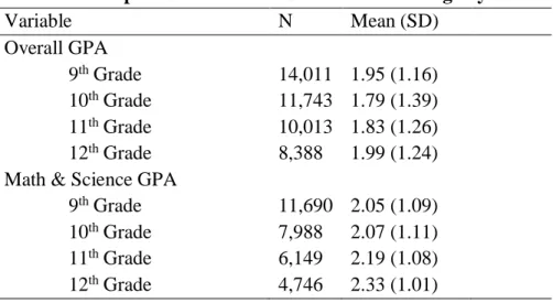
Table 1: Descriptive Statistics for Grade Point Average by Grade ... 43

Table 2: Descriptive Statistics for Attendance Variables by Grade ... 44

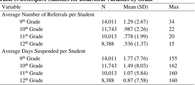
Table 3: Descriptive Statistics for Behavioral Variables by Grade ... 45

Table 4: Descriptive Statistics for Aggreagated Grade 12 Data ... 46

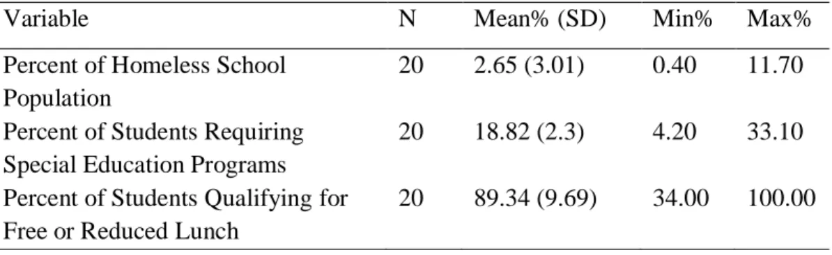
Table 5: Descriptive Statistics for School Level Homeless, Special Education, and Free/Reduced Lunch Variables ... 46

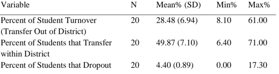
Table 6: Descriptive Statistics for School Level Turnover, Transfer within District, and Dropout Variables ... 48

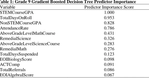
Table 7: Grade 9 Gradient Boosted Decision Tree Predictor Importance ... 60

Table 8: Variables Used in Model Development ... 101

Table 9: Grade 9 Gradient Boosted Decision Tree Model Performance Metrics ... 60

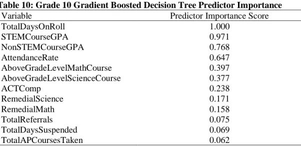
Table 10: Grade 10 Gradient Boosted Decision Tree Predictor Importance... 61

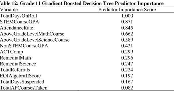
Table 11: Grade 10 Gradient Boosted Decision Tree Model Performance Metrics 62 Table 12: Grade 11 Gradient Boosted Decision Tree Predictor Importance... 63

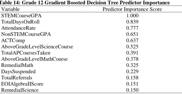
Table 13: Grade 11 Gradient Boosted Decision Tree Model Performance Metrics 63 Table 14: Grade 12 Gradient Boosted Decision Tree Predictor Importance... 64

Table 15: Grade 12 Gradient Boosted Decision Tree Model Performance Metrics 65 Table 16: Grade 9 Artificial Neural Network Global Sensitivity Analysis ... 66

Table 17: Grade 9 Artificial Neural Network Performance Metrics ... 67

Table 18: Grade 10 Artificial Neural Network Global Sensitivity Analysis... 68

Table 24: Grade 9 Multilevel Logistic Regression Results ... 72

Table 25: Grade 9 Multilevel Logistic Regression Performance Metrics ... 73

Table 32: Grade & Model Level Performance Metrics ... 78

Table 33: Artificial Neural Network Grade 9 Node Weights ... 103

(9)

viii

LIST OF FIGURES

Figure 1: Artificial Neural Network Sample Structure ... 14

Figure 2: GBDT Performance Metrics by Grade Level ... 81

Figure 3: ANN Performance Metrics by Grade Level ... 82

Figure 4: MLR Performance Metrics by Grade Level ... 83

(10)

ix

LIST OF EQUATONS

Equation 1: Basic Multi-layer Artificial Neural Network Function ... 15

Equation 2: Artificial Neural Network Single Node Error Term ... 17

Equation 3: CART Minimization Function for Variable Selection ... 20

Equation 4: Within Node Deviance Function ... 20

Equation 5: Decision Tree Node Fit ... 20

Equation 6: Multilevel Regression – Level 2 Function ... 24

Equation 7: Multilevel Regression – Level 1 Function ... 25

Equation 8: Model Accuracy ... 27

Equation 9: Model Sensitivity ... 27

Equation 10: Model Specificity ... 27

Equation 11: Model Precision ... 28

Equation 12: Matthews Correlation Coefficient ... 28

Equation 13: Average Multinomial Deviance for Boosted Trees ... 52

Equation 14: Global Variable Importance for Boosted Trees ... 53

Equation 15: Global Variable Importance with Unequal Classification Correction 53 Equation 16: Artificial Neural Network Node Deviance ... 55

Equation 17: Iterative Reduction of Deviance Function ... 55

Equation 18: Global Sensitivity Measure ... 55

Equation 19: Grade 9 Multilevel Logistic Regression Model ... 72

(11)

x

ABSTRACT

The use of data mining algorithms for applied practice is becoming

commonplace in many industries. The application of these models to the domain of educational data and practice could provide significant gains in understanding and implementation of prediction in the classroom. The wealth of data collected from students as they progress through a traditional education track could benefit greatly from machine learning and data mining. The present dissertation is designed to examine the usefulness, when compared to Multilevel Logistic Regression, of Artificial Neural Networks and Gradient Boosted Decision Trees, at predicting college enrollment using data collected as students progressed through high school. Because of the immense amount of data that data mining algorithms can interact with, the emphasis is placed on, but not limited to, variables representing difficulty of coursework, advanced placement, STEM vs non-STEM, behavioral referrals, attendance, and any statewide standardized testing. The grade level data was analyzed independently for each model to determine at what pace model predictive consistency increased as new and more relevant information was collected. The comparison of model predictive

capacity revealed that certain data mining algorithms could indeed be used in place of traditional statistical models, but the gains were not always consistent across all grade levels. Implications and future research are discussed.

(12)

1

CHAPTER I: INTRODUCTION

In recent years, many academic and applied fields have seen an onset of data mining & machine learning techniques being implemented into standard protocol (Han & Kamer, 2011). The emergence of large-scale, automated data collection combined with the new methods of making large data available has established a need for machine learning algorithms to parse through vast amounts of data. This marriage of technological advancements and the operationalization of computers in most daily activities has not only created an abundance of data, but also allowed for a greater body of available data across most domains.

Fields such as education, computer science, finance, health sciences,

production, and business have found ways to utilize data mining techniques for data extraction, data cleaning, and pattern recognition ultimately leading to faster, more efficient decision making (Hastie, Tibshirani, & Friedman, 2009). With this

abundance of large datasets, systems of analytic techniques and exploratory methods become a necessity to organize and display information in an intelligible, meaningful manner. This is the primary reason data mining has been extended beyond an available option and become a necessity in many instances. Many data mining implementations being used in large corporations also contain automated machine learning functions. These algorithms perform analytics and

decision/solution recommendation, but also have the capability to continually re-deploy analyses with every new data point gathered (Witten & Eibe, 2005). This allows the user to spend less time on optimization and maintenance of an analytic environment, while also permitting the machine component to continually

(13)

2

recalibrate weights for more optimized, relevant predictions. This continuous

process also allows the models to adapt to the data as the data might change (Stoean, Pruess, Stoean, El-Darzi & Dumitrescu, 2009).

The unique approach to model development when viewed with an

abundance of data is also one of the primary contributors that differentiates classical statistics from data mining and machine learning. The massive amounts of data becoming available in modern day systems allows for a much more exploratory approach to be implemented. Many data mining models place an emphasis on utilizing large quantities of data that, in many cases, could not be handled easily by common statistical techniques. Due to this strength of data mining models, it is common in data mining methodology to emphasize greatly understanding the

domain and data so to not generalize and over-fit a prediction model (Lavrac, 1999). Hastie et al. (2009) stated that the type of learning being done in data mining

referred broadly "to approaches that take a more inductive approach to building a model, allowing the data a greater role in suggesting the correct relationship between variables rather than imposing them a priori."

Specifically, in the realm of education, data mining is being implemented in unique situations, but not yet widespread in its application. One area of improved usage is in the measurement of unique student models for student classification (Ayala & Yano, 2009). The onset of data being gathered will now allow for unique models to be built at the student level, so learning systems can become more custom fit for individuals rather than clustered groups. Baker & Yacef (2009) anticipated that with the access and organization of large amounts of student level data,

(14)

3

machine learning algorithms can now be implemented to track and model students’ knowledge, motivation, disposition, as well as, many personality traits that impact a student’s educational journey. The move towards more machine-based assessments and computer adaptive measurement profiles is a by-product of a shift toward a more digital learning environment. Rupp, Nugent, & Nelson (2012) proposed that assessments are moving away from fixed-form stand-alone tests combined with short-form responses to robust adaptive assessment suites composed of

performance-based tasks administered collaboratively in digital learning environments.

Given the large amount of data being collected throughout a students’ academic progress, along with the standardized testing batteries being implemented at many milestones in a student’s academic career, the field of educational research has become inundated with data that is either not being utilized to its full advantage or not being used in conjunction with other important fields (Murtaugh, Burns, & Schuster, 1999). By adapting the machine learning algorithms developed for data mining in other domains to the realm of educational research, new pattern detection approaches can assist in sifting through large amounts of data (Cristianini & Shawe-Taylor, 200).

The current study centers around taking advantage of a multitude of educational data and seeking out reproducible patterns to enrich prediction of college enrollment. This was achieved by examining large amounts of data covering many domains of a student’s life and experience, and programmatically parsing

(15)

4

through it for identifiers indicating a higher probability of involvement in higher education.

The focus of this dissertation is not to prove machine learning algorithms have a place in educational research, because data mining has already impacted many facets of our national education system (Bhise, Thorat, & Supekar, 2013). The focus is instead to compare the predictive efficacy of the most commonly used machine learning algorithms when applied to the academic data commonly collected by state institutions. The uniqueness of this dissertation resides not only in the comparison of advanced methodology with more standardized statistical methods, but also the significance and breadth of the data collected for the analyses. A primary component of analysis will be a comparison to a more traditional statistical technique in use with most academic research. This measure is not intended to act as a baseline, but instead, one component of a general, unbiased comparison between prediction models.

The data being utilized for these analyses are significant due to, not only, the extended duration in which data collection took place (high school grades through early college years), but also the collection of multiple cohort years (3 separate cohorts) to control for any dependencies that could exist due to events occurring in a single academic year. This primed the data for a suitable comparative study,

examining the predictive accuracy of the three models that will be detailed in a later section.

(16)

5

CHAPTER II: LITERATURE REVIEW

2.1 - Description of Data Mining

Data mining carries many definitions based on what type of professional is using it, as well as, the reason in which it is being used. The realm of computer science would view data mining through a different lens than a marketing

researcher. Many of the definitions vary in terms of the amount of computational prowess versus the statistical methodology (Quinlan, 1986; Quinlan, 1993). When data mining began, computer scientists would primarily label it pattern detection using a series of algorithms, while the market researcher would view it as an analytic tool based more heavily in statistics than computer science (Shute, 1993). Pregibon (1996) provides one of the most universal definitions of data mining by stating that it is composed of three parts: statistics, artificial intelligence, and

database systems research. The extensiveness and generality of the definition is due, in part, to the many tools and techniques that all reside within the scope of data mining as a field. There are many data management and exploratory methods that would rely much more on the database research portion of the definition. In turn, there are classification tools that would rely much more heavily on the statistical portion of the definition. Overall, data mining is best described as a pseudo-automatic process by which potentially hidden patterns and relationships in information are discovered (Dorian, 1999).

Gorunescu (2011) states that data mining has three “generic roots” that make up the field. The first, and oldest, root is statistics. Statistics provides

(17)

6

pattern-oriented relationships between bodies of variables when there is no information about the nature of the variables (Tukey, 1977). The second “root”, artificial intelligence, is much more recent in origin than statistics. Artificial

intelligence takes a heuristic approach to problem solving, contributing information processing techniques to the data mining procedure (Gorunescu, 2011). Artificial intelligence is commonly labeled as Machine Learning in most applied analytic environments. The third “root” is database systems research. This is made up of techniques such as data acquisition, data cleaning, and data management (sub-setting, creation of new variables from multiple variables’ information, etc.), and provides the basis from which the information is mined (Witten & Eibe, 2005). Data mining can be dissected into two primary areas, similar to statistics, predictive objectives (e.g. continuous outcome prediction, classification, anomaly detection) and descriptive objectives (clustering, visual exploration, association rule development, sequential pattern detection). Within these two areas, many methods and practices exist surrounding key aspects of pattern detection and outcome prediction. The many models and algorithms available under the umbrella of data mining can be viewed as tools that the professional must implement based on the uniqueness of the data and desired outcome. One common trait in data mining, that spans across multiple concentrations and multiple theoretical backgrounds, is the idea of data mining as a series of very important steps that must be completed in a very strict order. Most institutions and organizations that utilize data mining recommend a specific methodology known as the Cross Industry Standard Process

(18)

7

for Data Mining (DM), but many areas use a modified version of CRISP-DM, usually merging or splitting the steps (Shearer, 2000).

2.2 CRISP – DM Methodology

CRISP-DM is constructed of six equally important steps. Business

Understanding, Data Understanding, Data Preparation, Modeling, Evaluation, and Deployment. During the Business Understanding step, the primary goal is to identify the project objectives. These objectives could include, but are not limited to, success criteria for tools or techniques, risks and contingencies, and project plan outcomes (Chapman et al., 2000).

The Data Understanding step involves collecting and reviewing the data. This could involve creating descriptive reports on data and reviewing the collection process, exploring the data, and data quality verification. The Data Preparation step includes selecting and cleaning the data. During this step, it is important to describe the rationale for including or excluding the data, creates reports describing the data cleaning methods utilized, create the analyzable datasets (subsetting, transposing, merging variables, etc.), and reformat variables to prepare for analysis (Chapman et al., 2000). This step is important to approach very carefully, because the orientation, format, and type of data might not be ready for the modeling step. If data cannot be analyzed properly, then the whole data mining process could provide improper or inaccurate results.

The Modeling step contains most of the statistical techniques and

assessments. The goal of this step is draw conclusions related to your goals set in the Business Understanding step. This could include, but is not limited to, creating

(19)

8

models, classifications, predictive measures, and assessment of the predictive measures implemented (Clifton & Thuraisingham, 2001). Model assessment is also a very important part of the Model step. Assessing the fit of parameters and revising parameters included in the model are both vital actions when building a model. This step usually consists of making judgments on the success of models when compared with each other, basing model assessment on the accuracy and appropriateness of model fit (Chapman et al., 2000).

The Evaluation step is similar to the assessment portion of the Model step. The model assessment being done in the previous step assessed the accuracy and generality of a model, while the Evaluation step assesses the degree to which the model meets the criteria established during the Business and Data understanding phases (Leaper, 2000). It is not until a model possesses good fit, and satisfies the standards and goals set forth by the researcher that it is accepted as an appropriate model. The final step is the Deployment step. This step is vital when utilizing data mining for the development of solutions in an applied setting. It involves applying the results of the data mining procedures and monitoring these changes to ensure that the proper decisions were made (Chapman et al., 2000). This study will not involve the use of the Deployment step. A future direction component will follow the final evaluation step, as this study is not designed in a way in which the conclusions could be brought into action.

These steps outline the basis for data mining and its ability to be implemented. Although the exact structure of CRISP-DM cannot be fully

(20)

9

utilized as closely as possible. The primary component that will guide this study is the utilization of supervised learning. Supervised learning is required in situations where there is no unique fit measure or acceptance test available for the utilized models. Supervised learning techniques incorporate every input variable into the initial analysis called the training model. This model is developed on only a portion of the data and done in such a way that the learning algorithm being used seeks suitable functions that relate the input variables and output variables. This allows the algorithm to see the input and output data simultaneously to develop a model that represents the relationship between the two. Where this practice differs from methods incorporated in traditional statistics is the model selection, error reduction, and input removal that takes place. Most data mining algorithms will train their model by creating hundreds, if not thousands, of unique models, testing them all, then selecting the model or models that recreate the data the best. Machine learning algorithms like artificial neural networks even back propagate during the modeling phase (Han, Kamber, & Pei, 2012). This allows the algorithm to move forwards and backwards through the series of input and output variables to iteratively test and retest weights applied, thus removing error with each estimate (Rumelhart, Hinton, & Williams, 1986). This will be discussed in greater detail at a later point in the study.

2.3 Data Mining in Education

Educational measurement has experienced a shift in focus from traditional graduation rates, to more attention focused on college readiness (Strauss & Volkwein, 2004). As the reality of an increase in students attending college or

(21)

10

university becomes more evident, it is vital to accurately measure how prepared students are for attending post-secondary school (Birnie-Lefcovitch & 2000). Although consensus agrees that college readiness is vital to understand, there still exists many opinions as to what factors actually contribute to college readiness (Conley, 2007). Desjardins & Lindsay (2008) state that in most cases, some combination of actual quantitative measurables (e.g. GPA, count of advanced courses taken, etc.) and designed assessments geared toward post-secondary school achievement provide valuable information for predicting college readiness. Data mining models provide a new set of tools to better investigate the many patterns that exist within educational data.

Due to the financial implications involved, data mining models are more commonly being implemented for predicting student enrollment in college, attrition due to intermittent circumstances, and key motivators university administration can control concerning enrollment expectations (Luan & Zhao, 2006; Brewe, Kramer & O’Brein, 2009; Delen, 2010; Herzog, 2006). There is also research taking place in areas with less financial impact on institutions. predicting academic differences that exist for distance learning students, focusing resources towards non-traditional students to lessen academic churn, and locating trends in drop-out and retention fluctuations of specific student type (Kotsiantis, Pierrakeas, & Pintelas 2004; Siraj & Abdoulah, 2009; Herrera, 2006).

It has not taken long for the practice of data mining and machine learning to become functional in the field of education, and this trend will only grow as more methodology and application become proven with research and practice. The

(22)

11

overarching methodology of data mining and the practices of data mining within the realm of education have been described. The primary focus of this study is to

provide a framework and comparison for how these models interact with a

traditional statistical model when viewing large-scale educational data. The focus will now turn to the specific models being implemented within the practice of data mining and machine learning.

(23)

12

CHAPTER III: METHODOLOGICAL REVIEW

3.1 Classification vs Prediction

Modeling with predictive data mining models can generate two primary outcomes, classification and prediction, principally determined by the data being analyzed and the model being implemented (Weiss, Kulikowski, 1991). The identification and purpose of the two model types is based on the format of the outcome variable being predicted and the unique needs that accompany the data being investigated. Classification describes the process of creating a function distinguishing data into various classes or levels. The outcome variable for a

classification model is always discrete and unordered. In contrast, prediction models do not classify into levels or categories, but instead model outputs made up of continuous outcomes, similar to multiple regression (Han, Kamber, and Pei, 2012). Prediction models are implemented to predict numerical data values rather than the discrete categories present in the classification output. Data mining in applied applications even allows the model to decide the proper outcome for prediction and form fit the model to best represent patterns accompanying that prediction.

Many types of data mining models (e.g. Classification and Regression Trees & Artificial Neural Networks) have the ability to perform as classification models and regressions models, with most models also allowing for both types of variable to be present as predictors (Alpaydin, 2011). Since one of the primary purposes of data mining as a practice is to detect reproducible patterns in data large enough that the signal is hardly detectable when compared to the noise, it is vital that the appropriate tool from the data mining toolbox is selected for the data.

(24)

13

The models selected for comparison in this study were selected based on the following criteria: presence in current research and experimentation, availability of software required for implementation, and the models most utilized in current applied practice. The two primary machine learning models selected to characterize data mining are Artificial Neural Networks and Boosted Trees (Gradient Boosted Regression Trees). To provide a baseline for comparison with more classically utilized statistics, Multilevel Logistic Regression will also be utilized to analyze the data.

3.2 Artificial Neural Networks

Cheng and Titterington (1994) summarized Artificial Neural Networks (ANNs) as “the mathematical models represented by a collection of simple

computational units interlinked by a system of connections.” ANNs can be viewed as a complex system of nonlinear relationships composed of hidden layers and intuitive learning mechanisms (Taylor, 1999). Hastie, et al. (1999) described ANNs as “A two-stage regression or classification model… [in which] the central idea is to extract linear combinations of the inputs as derived features, and then model the target as a nonlinear function of these features.” The use of ANN models allows for processing of many units of data that, when viewed together, seek out trends and relationships between input and output variables (Sibanda & Pretorius, 2012). Haykin (2008) described ANNS as a “biologically inspired analytical technique, capable of modeling extremely complex non-linear functions.” The biologically inspired component that Haykin mentioned comes from the architecture of the network when viewed from input to outcome. The ANN structure consists of

(25)

14

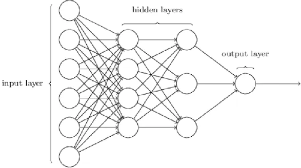
processing nodes that exist as inputs for the model, joined with “neurons” that are interconnected through groups of weights, similar to the synaptic connections located throughout the nervous system (Mehrotra, Mohan & Ranka, 1997). This architecture allows for a “signal” to flow from input to weights to output and in reverse order. In between each layer of the ANN, a complex set of nonlinear models communicate information through the layers until convergence occurs in the output layer (Bishop, 1995; Bishop, 2006). An image representing a sample ANN is presented in Figure 1 to show the structure of nodes and their relationships.

Figure 1: Artificial Neural Network Sample Structure

Within the ANN portrayed above, the input layer consists of the input variables included in the dataset, with each input variable representing a separate input neuron (Haykin, 2005). The hidden layers are created by the model to apply parameter weights to the layers of inputs (Singh, Parhar & Malla, 2015). Each input neuron can communicate with each hidden layer in a unique way, and any number

(26)

15

of input neurons can impact any number of hidden nodes within the hidden layers (Bishop, 1995; Funahashi & Nakamura, 1993; Webb, 1994).

When referring to the components of an ANN, the input variable or “input layer” is anything that is bringing some data or information into the model (Nowlan & Hinton, 1992). On the opposite end of the model, anything that holds a predicted value or weight is considered an “output layer.” There are also transformation functions nested in between the input and output layers that are called “hidden layers” (Luger & Stubblefield, 1993). As data flows from the input layer, through the hidden layers, and then continues on through the output layers, weights are assigned to each interconnecting line between two nodes (Sietsma & Dow, 1991). When the data reaches a hidden layer, the node (neuron) aggregates all values arriving from the input layer and the overall input values are applied to the model. Then the information is output to the next layer, where new weights are calculated and the process starts again (Sibanda & Pretorius, 2012; Neal, 1996).

Most applied ANN models are multi-layer network, which allow multiple inputs to be mapped to hidden nodes and output nodes with a series of complex non-linear relationships (Hastie et al., 2009). The basic function for a multi-layer ANN is: 𝑎𝑘 = 𝑔𝑘(𝑏𝑘+ ∑ 𝑔𝑗( 𝑏𝑗 + ∑ 𝑎𝑖𝑤𝑖𝑗 𝑖 ) 𝑤𝑗𝑘 𝑗 ) Equation 1 where 𝑎_𝑘is the output node, 𝑔_𝑘and 𝑔_𝑗are the activation functions that will change based on type of prediction being made (regression or classification), and 𝑏 is the bias (and weight decay if chosen to be included in the model). Bishop (1995)

(27)

16

recommends usage of nonlinear transformations in the hidden layers (e.g. tanh, sigmoid, logistic), due to the fact that multiple layers of linear transformations can be formulated in a single layer of computation fairly easily, and the primary goal is to take full advantage of the computational strengths of the network.

It is not a requirement that an ANN model only have one layer of hidden nodes (Bishop, 2006). The more layers within a network that exist allow for more levels of unique analysis containing the information carried from the previous layer. The issue of overfitting arises if networks become too complex and contain many levels of hidden nodes (Bishop, 1995; Ripley, 1996). When information is processed using an ANN, the network pushes the weights and bias obtained from the previous layer into the next node, allowing the algorithmic learning process to begin using the information processed in the previous layer (Mackay, 1995). This leads to very complex learning processes, especially once back-propagation is introduced and the data can flow back through the layers of the network (Neal, 1996). Models can be built with thresholds called weight decays from a programmatic standpoint, these will be discussed more at a later point. Back propagation and the bi-directional application in neural networks will be discussed in the next paragraph (Opper & Winther, 2000; Haykin, 2005).

The most commonly used ANNs can be classified into two categories, Feed Forward Neural Networks & Recurrent Neural Networks (Van de Cruys, 2014; Bishop, 2006). The main difference between how these two types of ANNs view data, is that Feed Forward Networks are not bi-directional, indicating a linear flow of data propagation from input variable to output variable. Recurrent Neural

(28)

17

Networks are bi-directional and allow for propagation of networks from later stages to earlier stages (Bitzer & Kiebel, 2012). When viewing Recurrent Neural

Networks, the most common estimation method is the Multi-Layer Perceptron (MLP) network. This network consists of at least 2 layers of nodes (neurons), input layer, output layer, and possibly hidden layers. MLPs are unique due to the way the model compares the output variables with known outcome values to calculate and apply a more accurate value of predefined error (Olden & Jackson, 2002). This error for the most basic neural network can be viewed as the following:

𝐸 = 0.5(𝑜 − 𝑡)2

Equation 2 where the error, E, is a function of the output value, o, and the target value, t. Once calculated, this error value is passed back through the network and adjusts the weights that have been applied to the models accordingly. This iterative process, called back-propagation, continues until a reduction in the overall error function is detected (Calcagno et. al. 2010). MLP is commonly accepted as the most functional and utilized ANN model due to the model’s ability to learn and re-estimate very quickly on large bodies of data. Research done by Hornik (1990) revealed that when presented with an appropriate amount of arbitrary data, MLP models are capable of deriving highly unique non-linear arbitrary models at very high accuracy levels.

Similar to other data mining algorithms that exist within a supervised learning environment, ANNs must be trained during use and implementation (Nilsson, 1990). Supervised learning is the practice of splitting the data to train the model being developed on one portion of the data and test the model parameters to determine successful classification using the other portion of data (Hastie,

(29)

18

Tibshirani, & Friedman, 2009). Mentioned briefly in the last section, the most commonly used training method in ANNs is back-propagation. During the process of information flowing from the input layer to the output layer, back propagation occurs to enhance predictive accuracy. Back propagation allows for information to pass back through the ANN with an adjusted expectancy of the error function. This allows for the weights being applied to the data to be adjusted as the models learns more about how the various layers relate (Weir, 1991). The primary goal of utilizing ANNs with this approach is to train a network that will find the best combination of variables and weights that produce the least amount of error when validated against similar data (Han et al., 2012). Validation is typically performed by randomly splitting the data and testing the model outcome on a portion of the data that wasn’t utilized for learning (Bishop, 1995). This validation method is also the most feasible method to use during this study due to the various types of models being

implemented. When implementing non-comparable modeling techniques fit

statistics commonly used in classical statistical theory are not applicable (Sietsma & Dow, 1991; Cawley & Talbot, 2007). This will be discussed in greater lengths during the methods section.

3.3 Boosted Decision Trees & Gradient Boosting

The second type of model that will be implemented in this study is the Boosted Tree model. The Boosted Tree model is a specific variation of the

Classification & Regression Tree (CART) model, which is typically the basis used for comparison for all decision trees (King & Resick, 2014). CART is the body of algorithms utilized within the field of decision tree. Decision tree will be explored

(30)

19

first, followed by an explanation of boosting and various optimizations that can be deployed with CART.

Decision trees are non-parametric, supervised modeling algorithms that can repeatedly run checks to extract the highest valued information from a dataset, without manual intervention, when presented with a model containing some predictors (Crockett, Latham, & Whitton, 2017). As stated is the case with many data mining models, decision trees can exist with categorical predictors

(classification trees) and continuous predictors (regression trees). Within the structure of the tree, there are root nodes, daughter nodes, and terminal nodes. The root nodes exist at the top of the tree and contain all of the data being used to build the model, the daughter nodes are the nodes that exist throughout the middle of the tree containing the algorithmically determined splits in the data, and the terminal nodes are the nodes at the bottom of the tree representing partitions in the data that cannot be split anymore (Breiman Friedman, Olshen, & Stone, 1984; Gorunescu, 2011).

CART models utilize recursive partitioning to fit non-linear relationships without any pre-processing or preparation of the data (Quinlan, 1986). Recursive partitioning collects all of the data in one node at the top of the tree and proceeds down creating splits in the data with additional nodes until the tree is fully formed (Strobl, Malley, & Tutz, 2009). The primary reasons that the partitioning ceases is either a lack of data or one of the stopping rules has been triggered. The splitting algorithm utilized in decision trees iterates through all predictor variables until the variable that creates the most unique separation in the sample is located (Friedman,

(31)

20

2001). The minimization function utilized to select which variable will be used for the split can be viewed as

𝑚𝑖𝑛 [𝑚𝑖𝑛 ∑(𝑦𝑖1− 𝑐1)2+ 𝑚𝑖𝑛 ∑(𝑦𝑖2− 𝑐2)2]

Equation 3 where 𝑦_𝑖1 is the value of the outcome variable in node 1, 𝑦_𝑖2 is the value of the outcome variable for node 2, 𝑐₁ is the predictor variable value of observation with membership to node 1, and 𝑐₂ is the predictor variable value of observation with membership to node 2 (Hastie et al., 2009; Quinlan, 1986).

The model attempts to locate splits that minimize the sum of squared difference between the values and the within node averages, then being summed across nodes that share a common parent node (Breiman, 2006). The greater the similarity two nodes’ values have leads to smaller sum of squared difference values. The most common measure for this heterogenous, within-node value is expressed with the following deviance value:

𝐷𝑚 = −2 ∑ 𝑛𝑖𝑗𝐿𝑁𝑝𝑖𝑗

Equation 4 where 𝑛_𝑖𝑗represents the total number of subjects from group I in node J, and 𝑝_𝑖𝑗 represents the proportion of subjects from group I in node J (Elith, Leathwick, & Hastie, 2008). This deviance value will increase as within-node heterogeneity increases, thus indicating a lower level of strength in the prediction of the split (Breiman et al, 1986). One common representation of fit for all decision trees is:

𝐷 = ∑ 𝐷_𝑚

(32)

21

The iterative process of analyzing the impact of each variable continues once the resulting nodes are as homogenous as achievable when speaking of membership to one group or another. This node creation and “splitting” of the data continues until the within-node heterogeneity of the outcome cannot experience any greater reduction in the deviance of the data. As mentioned above, one of the reasons trees discontinue splitting into additional nodes are stopping rules that are deployed to stop the model from growing too large and losing too much accuracy (Dorian, 1999). As the tree grows too deep, there could exist too many splits in the data disallowing a justified amount of data to exist in each terminal node. While a shallower tree will lead to outcomes that are too heterogeneous (Han, Kamber, & Pei, 2012). These two instances are examples of the need for stopping rules such as pruning. Pruning is an integral component of CART modeling and allows for the tree to maintain accuracy and generalizability (Alpaydin, 2011). There are many pruning mechanisms in place based on what software is utilized for calculation, but at their root they all perform the same task and that is overgrowing the tree, then pruning the terminal nodes back to an optimal size.

Classically developed decision trees offer one rigid path of decisions that can be limiting in scope due to the focus being decided earlier in the model

development process (Breiman et al., 1984). Due to increases in available software algorithms and computing power, decision trees have become much more versatile and less likely to hone in on one specific node split, causing the model to lose generalizability.

(33)

22

When Gradient Boosting is applied to the tree, creating a Boosted Tree, the concern of relying on a single rigid path is dissipated. The Gradient Boosting technique is an optimization technique that can be implemented for classification, regression, or rankings solutions (Brieman, 1998). Gradient Boosting leverages elements of Gradient Descent as well as Model Boosting. Gradient Descent being the process of minimizing an error function by moving in the opposite direction of the negative gradient (or residual), and Model Boosting being the process of adapting to a number of different loss functions with varying robustness to outliers (Freund & Schapire, 1996; Schapire & Freund, 2012). During this process, an ensemble, or additive, model is fitted in a forward step-wise progression. During each step, the model introduces what is called a “weak learner” that exists as a new weight that is meant to slightly improve on the weakest existing model component (Elith et al., 2012; Brieman, 1999).

The first successful boosting technique, Invent Adaboost, was implemented by Freund and Schapire (1997), but with a greater body of research, computational power, and data Gradient Boosting began to be developed in work by Friedman (2000). The “Gradient” component added to the algorithm was implemented to account for a large variety of loss functions (Friedman, Hastie, & Tibshirani, 2001). Gradient Boosting algorithms as they are used today, primarily compensate for residuals in a step-wise fashion so to continue reducing error by creating new nested regression or classification trees in ensemble models as the training data is analyzed (Friedman, 2002; Brieman, 1996).

(34)

23

3.4 Multilevel Logistic Regression

Multilevel modeling has historically been utilized to better predict outcomes in education related domains. This is due to the very natural hierarchy that comes about through the designation of students, schools, districts, regions, states, etc (Raudenbush & Byrk, 2012). The outcomes predicted by multilevel models can be oriented to focus on high levels and low levels within the data structure. When viewing the structure of a hierarchy, all levels that exist below a given level of the hierarchy are, by design, nested (Rocconi, 2013; Baeck & Van den Poel, 2012). These nested data structures will maintain high correlation with the structure that they are nested within. Due to this high correlation, regression models that assume independence of error and random sampling techniques are not appropriate (Singer, 1998). Standard errors can also be misestimated due to a failure to account for any dependence data might have on a higher-level structure within the hierarchy in which it is nested (Roberts, 2004). The assumptions that follow multilevel models account for the implicit relationship that exists between the levels of a nested hierarchy (Tabachnick & Fiddell, 2012).

Singer (1998) stated that one of the primary goals of utilizing multilevel modeling is to create functions of value at multiple levels of interest. When considering the current data set being analyzed, this would encompass functions directed at the school level, or second level, as well as, the student level, or first level. The data being utilized is limited to one school district, so there will be no need for a third level of hierarchy in the model implemented in this study.

(35)

24

The subsequent description of a use-case on the data collected for this study will aid in describing the relationship the levels of hierarchy have with the overall model. When examining the school level, one area of interest when utilizing multilevel modeling could be a categorical predictor for the academic level of a specific subject area offered at the school. In the data used for this study, consultation took place with the subject matter experts to grade, quantify, and standardize the “academic level” of the math, reading, and science courses offered at the various schools in the data set. After cleaning, this academic level field indicated if the math, science, or reading course being taken by the student (or offered at the school) was below the desired grade level, at the desired grade level, or above the desired grade level for the given school district.

If there is interest in modeling this at the school level to determine

probability of college enrollment, the mean predicted probability can be portrayed as a combination of the grand mean predictor (ϒ00), the selected impact the aggregate academic level course taken at the school (ϒ01) has on the predict

probability, the error associated with each individual school in the dataset (μ0j), and the error associated with the individual students in each classroom (rij).

ϒij = ϒ00 + ϒ01(Level) + μ0j + rij

Equation 6 The model above represents the school level function. If there was interest in adding to the overall model by examining the impact of total AP credits earned on the predicted probability of college enrollment, the student level model would be viewed as:

(36)

25

ϒij = B0j + B1j(APCREDITHOURS)ij + rij

Equation 7 with Β0j = ϒ00 + μ0j and Β1j = ϒ10 + μ1j. Once all of the functions are combined, the overall model would allow for better understanding of the influence of variables at both levels of the hierarchy, along with the errors unique to school and students levels of the model. Along with the unique errors represented in each level of the model, it is also of interest to explain the variance captured in the slopes (τ11), the variance captured in the intercepts (τ00), and the covariance between the two (τ01).

Multilevel modeling is not restricted to only prediction of continuous outcomes. This study is focused on predicting college enrollment, so the model will be applied to a dichotomous outcome. The basic principles of the model and its construction will still follow what was described above.

3.5 Model Comparison

The primary goal of this dissertation is to provide a comparison of the three models of interest within the context of large behavioral/educational datasets. The primary issue that arises when comparing the models’ ability to properly select college enrollment is the method of which each model uses to depict optimization or success. Logistic regression computationally follows the primary constructs of traditional statistics, while the data mining algorithms both utilize supervised learning to measure model accuracy, sensitivity, specificity, and precision (Breiman et al., 1984). Due to there being no common ground between how these two models are traditionally interpreted, all three models will be compared using a supervised learning environment (Ludbrook, 2002; Suleiman, Tight, & Quinn, 2016).

(37)

26

As mention before, supervised learning takes place when a smaller portion of the data set is randomly sampled to “train” the model and decide parameters, then the model with updated parameters is applied to the rest of the data to assess how well it predicted the known outcomes (Fay, 2005). Since this is the natural process that would take place for artificial neural networks and gradient boosted tree algorithms, the primary modification will take place with the multilevel logistic regression models. The multilevel logistic regression models will be trained on the same subsample as the other two models, then tested against the remaining data to assess model fit.

The four major components of model fit, when working within supervised learning states, are model accuracy, model sensitivity, model specificity, and model precision (Brieman et al., 1984). To understand these three metrics, it is important to first understand the four possible outcomes that can occur with a categorical

outcome. When trying to predict a dichotomous outcome like college enrollment, each observation of the test dataset can result in a True Positive (TP), False Positive (FP), True Negative (TN), or a False Negative (FN) (Jain & Zongker, 1997; Guyon & Elisseeff, 2003). A true positive would occur when the model correctly predicts a student enrolled in college. A false positive would occur when the model predicts a student will enroll in college, but that was not the outcome. A true negative would occur when the model correctly predicts a student not enrolling in college. A false negative would occur when the model predicts a student will not enroll in college, but that was not the outcome.

(38)

27

In gauging the overall Model Accuracy, or the model’s ability to

differentiate between students who would enroll and students who would not enroll, the proportion of true positives (TP) and true negatives (TN) from all evaluated observations must be calculated.

Accuracy = _{𝑇𝑃+𝑇𝑁+𝐹𝑃+𝐹𝑁}𝑇𝑃+𝑇𝑁

Equation 8 In gauging the overall Model Sensitivity, or the model’s ability to determine college enrollment properly (ignoring successful prediction of students not enrolling in college), the proportion of students who were correctly predicted as enrolled, true positives (TP), from the total number of students who did enroll, true positive (TP) and false negative (FN) is calculated.

Sensitivity = _{𝑇𝑃+𝐹𝑁}𝑇𝑃

Equation 9 In gauging the overall Model Specificity, or the model’s ability to properly predict students’ who did not enroll in college (ignoring successful prediction of students enrolling in college), the proportion of students who were correctly predicted as not enrolling in college, true negative (TN), from the total number of students who did not enroll in college, true negative (TN) and false positive (FP), is calculated.

Specificity = _{𝑇𝑁+𝐹𝑃}𝑇𝑁

Equation 10 Additional to the measure honing in on true positive rate (sensitivity) and true negative rate (specificity), it is important to also keep a measure of positive

(39)

28

predicted value, or Precision. This measure is captured as a ratio of true positives (TP) to true positives and false positives (FP).

Precision = _{𝑇𝑃+𝐹𝑃}𝑇𝑃

Equation 11 The final metric to consider when gauging the success of data mining

algorithms is the Matthews Correlation Coefficient, or phi coefficient in some literature (Boughorbel, Jarray, & El-Anbari, 2017). This metric is commonly deployed when a machine learning model is attempting to measure the quality of a binary classification predicted from a supervised learning environment and is widely accepted as one of the supervised learning measures of fit that is least altered by an inconsistent classification ratio (Matthews, 1975). It gains value because of its ability to maintain balanced outcomes when the class sizes in the data are of drastically different sizes (Powers, 2011). On occasion, it becomes less valuable to only view accuracy, or the proportion of correct predictions, because the size

difference between the two outcomes is drastically different (Perruchet & Peereman, 2004).

The MCC has a range of -1 to 1 where -1 indicates a fully incorrect binary classification, and 1 indicates a fully correct binary classification. The use of the MCC provides the most balanced gauge for how well classification models are performing. To calculate the MCC, it is necessary to utilize the prior calculations for true positive (TP), false positive (FP), true negative (TN), and false negative (FN).

MCC= 𝑇𝑃 × 𝑇𝑁−𝐹𝑃 × 𝐹𝑁

√(𝑇𝑃+𝐹𝑃)(𝑇𝑃+𝐹𝑁)(𝑇𝑁+𝐹𝑃)(𝑇𝑁+𝐹𝑁)

(40)

29

It is common, when working with data mining algorithms, for the above described metrics to be included in a table referenced as a confusion matrix (Kohavi and Provost, 1998; Caelen, 2017). Many advanced models include components called confusion-matrix based attribute selection, which allows the model to automatically adapt model weights and continue calibration on new data based on values derived from the confusion matrix (Ming, 2011; Ruuska, Hämäläinen, Kajava, Mughal, Matilainen, & Mononen, 2018). For the purpose of this

dissertation, the metrics will be utilized for reporting the best fitting models during the model comparison phase.

3.6 Summary

This section has provided an appropriate introduction to theories behind each of the three modeling techniques utilized in this dissertation. The section began by explaining classification versus prediction from a data mining stance. Next, the processes involved in the implementation of an artificial neural network, gradient boosted tree algorithm, and multilevel logistic regression model were described. Lastly, the metrics used to compare the models and the process for which they will be compared is described.

Now that the use and theory of the data mining algorithms and multilevel models have been described, a greater emphasis will be placed on explaining the primary methods employed for data acquisition and data preparation/cleaning.

(41)

30

CHAPTER IV: EXPLANATION OF DATA AND

VARIABLES

4.1 Data Procurement

The data used for this study was acquired through and approved by work done with the University of Oklahoma. The high school level data, representing a large midwestern school system, was provided by the State Department of

Education and was combined with the appropriate college level data from the corresponding state’s higher education institutions. The joining of these datasets was completed by specialists designated through and approved by the University of Oklahoma, and multiple checks were put in place during the joining of the data so that purity was maintained. Required fields for matching were extended beyond just unique student ID, into such things as social security number, birthdate, birth year, and complete name. It was required that the two data files match on at least 80% of the matching fields or the observation was excluded.

The master dataset originally obtained for this study contained 32,435 variables and 19,728 observations, totaling approximately 640 million data points. This initial dataset was made up of 3 cohorts of students who attended school in the large midwestern school system. The data spans from 6th_{grade through 12}th_{grade at} the individual student level with fields for every recordable action throughout the students’ academic career. The data also includes all alternative schools, magnet schools, and behavioral schools. Once the three cohorts were merged, the dataset was then combined with the corresponding college level dataset collected by the State Regents for Higher Education.

(42)

31

The methods implemented for matching the school level data with the college level data were validated internally by the State Regents for Higher

Education and any non-matching cases were removed from the sample. The criteria for matching included social security number, first name, middle initial, last name, and date of birth. To be included in the dataset, each observation (student) was required to match on an established number of these criteria, all of which were set and validated by the State Regents for Higher Education before delivery of the data.

4.2 Data & Variables

As mentioned above, the dataset contained 32,435 variables, so each variable will not be explained in detail. This was due in part to how the data was collected and stored, creating a new variable for every possible grade level – record – student combination. The format of the variables and what was done to clean and process the data are discussed below in the Data Preparation section. Within the data, there were a number of naturally occurring subgroups. These subgroups were composed of Demographic fields, Academic fields, Behavioral fields, Social fields, and Enrollment/Attendance. The primary fields of interest from each of these subgroups will be explained below.

The Demographic subgroup contained sex, ethnicity, English as a Second Language (ESL), English Language Learners (ELL) resident status, homeless status, free/reduced lunch, special education classifications, physical impairment, other disability, and gifted & talented.

The Academic subgroup contained test scores such as EOI, CRT, OCCT, ACT, SAT, EXPLORE, and WIDA. Other Academic variables are GPA, Advanced

(43)

32

Placement courses taken, Advanced Placement credits earned, promotion, retention, benchmark test scores by subject, and credits earned. The EOI/OCCT variables were such things as content area of exam, raw and scaled scores, performance level, duration of student enrollment, English proficiency, and a flag for students taking the exam a second time due to unsatisfactory scores the first administration. Specific Academic variables were then created to add special focus to the analyses. A

variable representing Cumulative Math GPA was calculated by coding GPA at the course level and only keeping math courses.

There was also a detailed effort to create and code variables representing the course level of the math and science courses offered. Subject matter experts

associated with and approved by the University of Oklahoma, specializing in the courses being viewed, contributed information to this classification process based on course number at each respective school, as well as, the expected prerequisites for each course. They were classified as below expected course level (remedial), at expected course level, or above expected course level (AP, Honors, higher level math and science, concurrent enrollment) for each grade in the data. These variables were used to conceptualize the difficulty of the given math or science course in relationship to what the expected difficulty would be. These variables were created by first creating a list of every possible course name and course number from any public school included in the dataset (6th_-12th_{grade). After the compilation of the} course information, each course on the lists (one list for math courses and one for science courses) were coded in the given subject. The codes given represented one of the three groups mentioned above: below grade level, at grade level, or above

(44)

33

grade level, for each grade in the dataset. This information was then entered into the master dataset.

In calculating the STEM course GPA, a list of STEM course numbers were collected from the OSRHE. This list contained 109 courses that were deemed STEM courses by OSHRE. OSHRE was also responsible for denoting the coding scheme for Institution Type. This included Large State Research Universities (e.g. OU, OSU), Small State Colleges (e.g. UCO, SWOSU), and Community Colleges (e.g. OCCC, TCC). The calculation of the non-stem course GPA utilized the same list but controlled for the STEM courses and removed them from the aggregation.

The variables included in the Behavioral subgroup included things such as items from the EXPLORE test, items from the PLAN test, and items from the ENGAGE test. These items gauged things such as academic interest, willingness to put forth effort in school, details about post-high school plans, homework, family involvement in education, and perceived success. The Behavioral dataset also included variables on disciplinary action taken against the student. These variables included total number of referrals, type of referrals, total days suspended, reason for suspension, and number of truancies.

The variables included in the Social subgroup included primarily items collected from the ENGAGE test. This included items such as social connection with school personnel, managing goals, motivation, self-confidence, and

determination to succeed. The variables in the Enrollment/Attendance subgroup included school attended, number of times primarily school changed during year, school at which state test was taken, time of entry at each school, time of exit at

(45)

34

each school, reason for exit, absences per school, total absences, days enrolled per school, total days enrolled, and attendance ratio per entire grade year. There were a number of higher-education variables that were included in the predictor side of the dataset, primarily as controls. Examples of these variables are type of higher-education institution, student status (full time or part time), and STEM GPA. The primary outcome variable of interest that was included with the higher-education data set was enrollment/retention within a higher education institution.

There was also a school level dataset created from the aggregation of student level data with the associated school code. This school level dataset was matched against statistics provided by the State Department of Education for each school for validation purposes. The aggregate values matched with a minimal expected amount of error due to uncontrollable factors such as students transferring to other schools during the school year, students being relocated to behaviorally centered programs during the year, and students experiencing multiple instances of extended out of school suspension or expulsion. It was determined that, for the purpose of this study, there was an acceptable amount of variance between the values reported on the state documentation and the actual aggregate values. Since the purpose of the study is predicting college enrollment, school level data that was negatively affected by students primarily experiencing behavioral interventions would be discernable in the Specificity metric of each model.

The second level dataset contained predominately academic, behavioral, and demographic variables representing the schools captured within the dataset.

(46)

35

GPA, average student test performance (e.g. EOI, ACT, SAT), average number of AP courses taken, average promotion/retention rate, average graduation rate, average attendance ratio, average number of suspensions, and average number of disciplinary referrals.

4.3 Data Preparation

The data preparation portion of the study was difficult due to the orientation of the dataset. The data was combined so that one student was represented by one observation line in the dataset. This was difficult primarily because grade level data were not separated into grade subgroups. Each student had a year of entry for each school and a numeric coding scheme made up of underscores and numbers that would place each test score, behavioral instance, course taken, etc. into a specific year within the student’s academic career. Because of this coding scheme, a

student’s data under the variable titled GPA_2_2 (the first numeral representing the year and the second numeral representing the semester) that represented the

students’ cumulative GPA taken at the second semester of the 7th_{grade (because the} 6th_{grade was the first grade in the dataset and the _2 represents the second year).} Another student’s data under the variable GPA_2_2 could represent the student’s cumulative GPA taken at the second semester of the 11th_{grade (because the student} transferred into the school system in the 10th_{grade and the _2 represents the}

student’s second year in the dataset). This caused for additional coding to be written for each combination of every variable type and every grade/year combination.

Another aspect of the data cleaning effort was computing descriptive statistics and creating flags for variables containing cases that fell outside of the

(47)

36

defined range. There were 33 cases that contained variables with data that was out of range. Due to the importance of the variables that were out of range, the entire case was removed from analysis for each of these observations. After coding to recognize which variables placed students in grades, the primary dataset was split into seven grade level datasets. Each of these seven datasets contained one

observation for each student who recorded data in that grade. Students who did not have recorded academic, behavioral, or higher education data were removed from the dataset. Due to how the datasets were constructed, students who did not have grade level data but still had an identifying number were removed from the dataset. Duplicate case filters were added to each grade to ensure each student was not improperly represented in a grade more than once. This process will be discussed at greater length during the next section.

Data reduction methods were also used to improve the analysis phase of the study. There were groups of variables removed that did not pertain to every dataset. The variables were mainly characterized by complete blocks of missing data, but the data dictionary was used to validate the removal. These variables were checked to ensure no data existed for the irrelevant grade level datasets, and then removed from the datasets. An example of this type of variable would be one containing an item from a standardized test administered in the 8th_{grade, but due to the structure of the} dataset, the variable existed at each grade level. These variables would appear completely missing for a student in the 12th_{grade, because 12}th_{grade students did} not take a test administered to 8th_{grade students.}