Classifier Evaluation With Proper Scoring Rules

UNIVERSITY OF TARTU

Institute of Computer Science

Computer Science Curriculum

Diana Grygorian

Classifier Evaluation

With Proper Scoring Rules

Master’s Thesis (30 ECTS)

Supervisor: Meelis Kull, PhD

Classifier Evaluation With Proper Scoring Rules

Abstract:Classification is a fundamental task in machine learning, which involves predicting the class of a data instance based on a set of features. Performance of a classifier can be measured using a loss function, which assigns a loss value for each classification error.

Classification error happens when the predicted and the actual class differ. In the simplest case, all combinations resulting in a classification error are consid-ered equal in terms of cost. However, some problems demand different types of misclassification to be of different importance, which forms a cost context.

Depending on the properties of the cost contexts, different loss functions can be applied. For example, if the arithmetic mean of costs for one false positive and one false negative is fixed and these costs are uniformly distributed, then Brier score is the suitable loss function. If their harmonic mean is fixed, then log loss should be used instead. These two functions belong to a larger family of loss functions known as proper scoring rules. Scoring rules are loss functions which deal specifically with probabilistic classification, where the classifier is required to predict probability for each class, indicating prediction confidence.

In this thesis, a new cost context for binary classification is presented, where both costs have their own uniform distributions. A corresponding new loss function for this cost context is proposed, named Inverse Score, and is subsequently proven to be a proper scoring rule.

The experiments confirm that the total cost when using said cost context and expected loss when using the new loss function are the same.

Keywords: machine learning, classifier evaluation, probabilistic classification, proper scoring rules, cost-sensitive learning

Klassifikaatorite hindamine kohaste skoorimisreeglitega

Lühikokkuvõte:Üks põhilisi ülesandeid masinõppes on klassifitseerimine, mis seisneb andmepunktile kategoorse väärtuse ennustamises teatud tunnuste alusel. Klassifitseerija sooritusvõimet saab mõõta kaofunktsiooni abil, mis omistab igale klassitsifeerimisel tehtud veale mingi väärtuse.

Klassifitseerimisveaks nimetatakse olukorda, kus ennustatud kategoorne väär-tus on erinev sellest, mis peaks olema tegelik väärväär-tus. Kõige lihtsam on käsitleda kõikvõimalikke klassifitseerimisvigu võrdse kuluga. Siiski, mõndade probleemide lahendamine nõuab erinevat tüüpi klassifitseerimisvigadele erineva kaalu omista-mist, ning see moodustab kaokonteksti.

Olenevalt kaokontekstist on võimalik rakendada erinevaid kaofunktsioone. Näiteks, kui ühe valepositiivse ja ühe valenegatiivse hindade aritmeetiline kesk-mine on fikseeritud ning mõlemad on ühtlaselt jaotunud, sobib kaofunktsiooniks Brier’i skoor. Kui nende harmooniline keskmine on fikseeritud, sobib selle asemel kasutada logaritmilist kaofunktsiooni. Need kaks funktsiooni kuuluvad suuremas-se kaofunktsioonide perekonda, mida tuntaksuuremas-se kohaste skoorimisreeglite nime all. Skoorimisreeglid on kaofunktsioonid mis tegelevad spetsiifiliselt tõenäosusliku klassifitseerimisega, kus klassifitseerijalt on oodatud iga kategooria tõenäosuse ennustamist, kus tõenäosus omakorda näitab kindlust ennustatud kategoorias.

Antud magistritöös esitletakse uut kaokonteksti binaarsele klassifitseerimisele, kus kummalgi klassil on sõltumatult ühtlane jaotus. Nimetatud kaokontekstile pakutakse välja uus kaofunktsioon nimega Pöördskoor ning selle puhul tõestatakse, et see on kohane skoorimisreegel.

Eksperimendid kinnitavad, et kogukulu vastavas kaokontekstis ning oodatud kadu kasutades uut kaofunktsiooni on samad.

Võtmesõnad:masinõpe, klassifikaatorite hindamine, tõenäosuslik klassifitseeri-mine, kohased skoorimisreeglid, hinnatundlik õpe

Contents

1 Introduction 5

2 Classifier Evaluation 7

2.1 Types of Classifiers . . . 7 2.2 Basic Evaluation Measurements . . . 8 2.3 Cost-Sensitive Classification . . . 11

3 Proper Scoring Rules 18

3.1 Properness . . . 20 3.2 Numerical Example . . . 22 3.3 Bregman Divergences . . . 24

4 Derivation of Proper Scoring Rules 28

4.1 Brier Score . . . 28 4.2 Inverse Score . . . 32 4.3 Possible Generalization of Inverse Score . . . 38

5 Experiments 39 5.1 Setup . . . 39 5.2 Results . . . 40 6 Conclusion 41 References 44 Appendix 45 I. Code . . . 45 II. Licence . . . 45

1

Introduction

Classificationis the task of given an instance of data predicting its class from a fixed set of options. An instance is defined through itsfeatures, denoted byx, an its correspondingclass, denoted by y. For example, one can consider a classification task of predicting whether a given image is of a chihuahua or of a blueberry muffin. The set of features are all the pixels in the image. Feature space, denoted by X, is composed by all the possible images of given image size. Label space, denoted by

Y, consists of two labels: ‘chihuahua’ and ‘muffin’ [Yao, 2017].

Classifier evaluationis a task of measuring how good classifier is at labelling data. According to the ‘no free lunch’ (NFL) theorem [Wolpert, 1996], there is no universal learning algorithm that would work best for every problem. Therefore, for different datasets different algorithms (classifiers) perform with variable success. This means that for each task and dataset classifiers need to be reviewed and evaluated separately. That is why classifier evaluation is a crucial task in machine learning [Tharwat, 2018].

Loss functionis a type of classification evaluation measurement. It is a non-negative function that maps a pair of predicted and actual class to a real number, where higher values correspond to worse predictions while 0 indicates perfect classification.

Binary classification is a particular type of classification problems where there are only 2 classes, which are usually referred to as positiveandnegative. This allows for 2 cases of misclassification: false negative (predicting negative when the actual class is positive) andfalse positive(predicting positive when the actual class is negative). Most of the time, these errors are of different importance, and to highlight these differences parameters called costs are used. For binary classification, there are only 2 costs: cost of false negative, denoted by c0, and cost

of false positive, denoted byc₁ [Elkan, 2001].

Evaluation is complicated by the fact that models learn and work in different contexts. A context is defined by a set of parameters, such as cost magnitude, proportion of different costs, proportion of instances of different classes. Such contexts are calledoperating condition. Evaluating model in a concrete operat-ing condition is a trivial task. In case information about operatoperat-ing condition is unavailable, a model needs to be evaluated over a range of operating conditions [Hernández-Orallo et al., 2012]. Loss functions applicable to such problems are calledproper scoring rules. The most commonly used examples of proper scoring rules are Brier score and log-loss [Brier, 1950] [Good, 1952].

An operating condition, where the sum of costs is fixed, one cost,c₀, has uniform distribution and the other one,c1, can be calculated from the sum andc0, is called

additive. It was shown that Brier score produces correct expected loss when used with additive context [Hernández-Orallo et al., 2011]. A similar operating

condition where instead the harmonic mean of costs is fixed, one cost, c₀, has uniform distribution and another one, c₁, can be calculated from the harmonic mean andc₀, is calledharmonic, and it was proven that log-loss is equal to expected loss under harmonic context [Flach, 2015].

In this thesis, a new context is proposed, where both costs c₀ and c₁ have uniform distribution. Since in this case there is no correlation between c₀ and

c₁, this context will be called independent uniform. A score was found that is equal to total cost underindependent uniformcost context and its correctness and properness is proven. This score will be calledInverse Score.

In Section 2, types of classification and their evaluation will be introduced, and cost-sensitive learning will be discussed.

In Section 3, proper scoring rules will be reviewed, some examples of them are shown and their properness is proven, and Bregman divergences and their connection to proper scoring rules are introduced with some examples.

In Section 4, independent cost context and its appropriate proper scoring rule Inverse Score are defined and the theorems about correctness and properness are proven.

In Section 5, the results of experiments are displayed and analyzed. In Section 6, the thesis is concluded.

2

Classifier Evaluation

A classifier, orclassification model, is a function that implements classification, so its input is a list of instance’s features, and its output is predicted class [Hernández-Orallo et al., 2012].

In this section, different types of classification models will be discussed and their assessment methods will be introduced.

2.1

Types of Classifiers

Labelling Classifier Labelling classifier model is a function that produces a predicted class, given an instance with set of values called features. For a concrete instance, its features are denoted by x and its label as y. Then, feature space is set of possible features, denoted by X, and label space is set of all possible labels to chose from, denoted byY. In this thesis, classification with 2 labels will be discussed unless stated otherwise. Such classification is called binary. For binary classification, class 0 will represent positive class and class 1 will represent negative one. Following [Hernández-Orallo et al., 2012] and [Hand, 2009], it has notational advantages. ThenY ={0, 1}.

Probabilistic Classifier A probabilistic classifier is a mapping ˆp:X→[0, 1], where ˆpis a vector of probabilities of getting each class, ˆp=( ˆp₁, ..., ˆp_k). Probabil-ities of all classed add up to one, Pk

i=1pˆi=1. In binary classification, ascore pˆ

specifies how likely instancexis of class 1, with higher value of ˆpmeaning more likely, ˆp_≈P(Y ₌1|X ₌x). And 1−pˆ specifies how likely instancex is of class 0, 1−pˆ_≈P(Y ₌0|X₌x).

Probabilistic classifier gains labels from scores using adecision rule. The most common decision rule uses athreshold t, so instances with scores ˆp_>twould be predicted as of class 1, and as of class 0 otherwise [Hernández-Orallo et al., 2011]. To discuss what value threshold should have, we need to review calibration first.

For example, for a fixed instance model produces probability ˆp₌0.9 of being of negative class. A model is called well-calibrated, if for all such instances with probability ˆp=0.9=90% approximately 90% of them are actually of negative class. It is very unlikely for the proportion of negative instances to be exactly 0.9, but the closer proportion of negative instances is to probability, the better calibrated it is. So, probability estimator is calibrated if among all instances where the model predicts ( ˆp₁, ..., ˆp_k) the actual class distribution is also ( ˆp₁, ..., ˆp_k).

If model is calibrated, then a threshold should be such value that means that class that has a bigger probability should be predicted. To predict negative class that has probability ˆp, the following inequality needs to be satisfied:

ˆ

p_>1−pˆ 2 ˆp_>1 ˆ

p>0.5

Thus, model will predict class 1 if probability ˆpis more than 0.5, which means that decision thresholdtist₌0.5. So, model will predict class 1 if ˆp_>tand class 0 otherwise.

We will call probabilistic classifiercalibratedbecause it produces a value that is always in range [0; 1]. A scores does not have such restrictions; it can have any range, where higher value will mean more likely of negative class 1 and lower value will mean more likely of positive class 0. Such score will be termeduncalibrated. We will discuss uncalibrated scores, their calibration to probabilistic scores and decision rules in Section 2.2.

2.2

Basic Evaluation Measurements

Accuracy and Error Rate Accuracyis primary tool used for classification eval-uation and is equal to proportion of correctly predicted instances. It is obvious that accuracy has values in range [0; 1], and higher accuracy (closer to 1) means good classification and lower accuracy (closer 0) means worse.

Error rateis another measurement and it is equal to proportion of incorrectly predicted instances. It is a complement of accuracy, err₌1−acc, and lower error rate means better than higher error rate.

Accuracy and error rate are not the best tool, because they do not evaluate classes separately. In real world, classes are sometimes highly imbalanced. It is common that negative class represents ordinary instances, and positive class means in some way ‘outstanding’ and therefore interesting instance. In such cases negative instances outweigh positive instances, and developer is interested in predicting positive instances correctly.

Consider online advertisement as an example, where a developer needs to predict which users will click on the ad. Then, negative instance means that user did not click on ad and positive click means user did. Most people do not click on the ads, so a good click-through rate (proportion of positive class) is only 2%, which means that classes are highly imbalanced [Volovich, 2019]. It is obvious that a developer is more interested to find users who would click rather than not, so positive class is more important and prediction for positive class needs to be more precise.

And accuracy fails this task: if classes are imbalanced enough, positive predic-tion can be neglected altogether without losing high accuracy. Similarly, error rate can ignore a rare class as well.

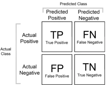
Figure 1. Confusion matrix for binary classification. Each entry in a cell is a count of instances with such prediction.

Figure 2. Cost matrix for binary classification. Each entry in a cell is a cost of prediction of certain instance.

Metrics for Imbalanced Classes In Figure 1, there is a confusion matrix, which is used to calculate most of common evaluation metrics. There are 4 possible cases for a single instance. If instance is predicted positive and is actually of positive class, then it istrue positive (TP). If instance is predicted negative and is actually positive, then it isfalse negative (FN). Similarly, if instance is actually negative and is predicted positive or negative, it is false positive (FP) or true negative (TN), respectively.

In such cases,precisionandrecallare pretty useful, since they focus on predict-ing positive class (the rare one) correctly. Precision, also called positive predicted value, is equal to _{T P}T P_{+F P}, and recall, in also called true positive rate, is equal to

T P

T P+F N [Tharwat, 2018] [Fawcett, 2005] .

There are many more classification evaluation measurements, like, for example,

F₁score, which is harmonic mean between precision and recall, orInformedness, that takes into account true positive and true negative rates. Every one of them is useful and could be an ultimate way to measure adequacy of some models if classification is not complicated further [Fawcett, 2015] [Powers, 2011].

Loss Functions The previous paragraphs gave a lot of examples of evaluations where higher result (closer to 1) is better and lower result (closer to 0) is worse. However, that is not always the case, and there are a lot of measures for which 0 is the perfect result and more is bad result. Such measures are called loss measures, or, more commonly, loss functions.

Aloss function(or cost function) for probabilistic classifiers is a non-negative function that takes as an input model’s score of an instance and instance’s actual label, and outputs a real number. Low value of loss function indicates better result, with 0 indicating perfect match between a prediction and instance’s label. The goal for optimization is to minimize the loss function.

Error rate was already introduced earlier and it is one of the easiest loss functions, and is equal to the proportion of incorrectly predicted instances. Most of loss functions are more complex than that as they are based on probabilistic classifiers rather than labelling ones.

Bayes-Optimal Model The best possible model is calledBayes-optimal model, denoted byp∗(x),p∗(x)=¡p∗₁(x), ...,p∗

k(x)

¢

, where p∗

i(x)=P(Y =i|X =x). That is,

for each instance, it produces probabilities of getting every label, given instance’s features. This model is theoretical and cannot be learned.

For binary classification, we will have classes 0 and 1, and only one probability

p will be used: p₌p∗₁(x) will mean probability of class 1 and 1−p₌p∗₀(x) will mean probability of class 0. Bayes-optimal is perfectly calibrated, which means it has threshold t₌0.5:

p∗₁(x)>p∗₀(x)

p_>1−p

2p>1

p>0.5

2.3

Cost-Sensitive Classification

As it was already discussed in Section 2.2, false negatives and false positive errors need to be taken into account separately. Moreover, it is common that one kind of error (usually false negative) is worse than another. For example, a bank needs to find from client’s transactions unusual (possibly fraud) transactions. Let the usual transactions be of negative class and unusual ones be of positive class. Then, it is a much bigger problem of classifying fraud as usual payment (and missing theft) than it is to classify casualty as fraud (a client would simply confirm their transaction and payment will go through) [Sun et al., 2011]. To indicate such differences in importance, there is set of parameters calledcosts, which is a measure of how bad consequences of a certain prediction is.

The general assumption about cost-sensitive classification is that the cost does not depend on the instance itself but rather on its class. Therefore, costs are usually represented as cost matrices for simplicity, and an example of cost matrix for binary case is visualized in Figure 2.

Cost C(i,j) stands for cost of predicting class iwhen the actual class is j. It is common for right predictions to not be penalized at all; therefore it will be assumed that C(0, 0)=0 and C(1, 1)=0. Negative values of costs will not be explored in this work. Conceptually, cost of misclassification should always be greater than predicting correctly. Mathematically, C(0, 1)>C(1, 1)⇒C(0, 1)>0 andC(1, 0)>C(0, 0)⇒C(1, 1)>0. These conditions are called thereasonableness

conditions [Elkan, 2001].

For simpler representation,C(0, 1) (false positive) will be further denoted as c₁

andC(1, 0) (false negative) will be denoted asc₀, where indexes of c₀, c₁ denote the actual class.

Values (or distributions) of all costs are calledcost context.

Cost-Sensitive Bayes-Optimal Model Bayes-Optimal model was already briefly discussed in Section 2.2. It was claimed that most of the times it uses threshold

t₌0.5. However, for cost-sensitive learning there will be different threshold. Probability of getting class 1 is p1= p and probability of getting class 0 is

probabilities are multiplied by respective costs, p₁c_1>p₀c₀: p₁c_1>p₀c₀ pc_1>(1−p)c₀ pc_1>c₀₋pc₀ pc₁₊pc_0>c₀ p_> c0 c₀₊c₁

Thus, classifier will predict class 1 if probability pis bigger than c0

c0+c1. That means

that cost-sensitive threshold ist=_c0c0_+c1.

Probability Density Function, Cumulative Distribution Function Accord-ing to the notation in Section 2.1, positive class is denoted by 0 and negative class is denoted by 1.

Probability density function (p.d.f.) for probabilistic scoressof class 0 is denoted by f₀(s), and cumulative distribution function (c.d.f.) is denoted by F₀(s).

Defined integral of p.d.f under limits [a;b], Rb

a f0(s)ds means probability of

getting scoresin range [a;b],a_<s_<b.

And c.d.f at value t,F₀(t)=R_−∞t f₀(s)ds, means probability of gettings in range [−∞;t], or simply less than t,s<t.

If tis a threshold, thenF₀(t) describes all the positive instances which scores are less than the threshold. Positive instances below the threshold will be classified as positive; that means thatF₀(t) is probability of positive instances to be predicted as positive, which is true positive rate, F₀(t)=T P/P os, where T P is expected number of true positive instances andP osis actual number of all positive instances. Following that, true negative rate is a complement of true positive rate, which means true negative rate is equal to (1−F₀(t)).

Similarly, F₁(t) describes all the negative instances which scores are less than the threshold t. Negative instances below the threshold will be classified as positive, which makesF₁(t) false positive rate,F₁(t)=F P/N e g, whereF P stands for expected number of false positives andN e gis actual number of all negative instances.

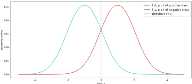
Lower scores are more likely to be of positive class 0, and greater scores are more likely to be of class 1. Let this relationship be described by two normal distributions, as shown in Figure 3. For positive class, f₀∼ N(−1, 1) and for negative class f_1∼ N(1, 1). The same distributions for scores of positive and negative classes will also be used in experiments in Section 5.

Figure 3. Probability density functions of scoressfor positive and negative class f₀

and f₁, respectively. Threshold is t₌0 because classes are calibrated and have the same cost.

Figure 4. Probability density functions of scoress for positive and negative class

f₀ and f₁, respectively. Threshold is t₌(ln 9)/2≈1.1 because class errors are of different cost,c₀₌9c₁.

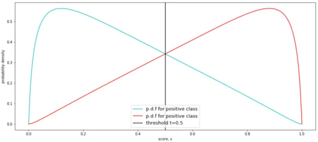
Figure 5. Probability density functions of probabilistic pfor positive and negative classes. Threshold is t₌0.5 because classes are calibrated and have the same cost.

Figure 6. Probability density functions of probabilistic scores pfor positive and negative classes. Threshold is t₌ c0

c0+c1 =0.9 because class errors are of different

and in Figure 3 costs for false positives are nine times bigger than costs of false negatives,c₀=9c₁.

Threshold tcan be calculated two ways, and the first is to scale scoressinto probabilistic scores pin range [0; 1], using perfect calibration map:

p₌ 1

1+e−2s

Such threshold will be denoted by t_p. For first case where costs are of the same value, threshold for probabilistic scoresswill betp=0.5 because data is calibrated,

as shown in Figure 5.

To avoid confusion, for uncalibrated scores s, threshold will be denoted by

ts. Threshold tswould be such value that satisfies equality f0(ts)= f1(ts). This

threshold ist_s=0, as shown in plot in Figure 3.

Now let us take a look at case where costs are different, c₀₌9c₁. For proba-bilistic scores a threshold can be calculated using the following formula:

t_p= c0 c0+c1=

9c₁

9c1+c1 =

0.9

And this result is shown in Figure 6. And for original scores swith distributions f₀

and f1it is such tsthat satisfies the equation:

f₀(t_s)

f₀(t_s)+f₁(t_s)=

c₀ c₀₊c₁

In this particular case with cost contextc₀₌9c₁and densities f_0∼ N(−1, 1) for positive class and f_1∼ N(1, 1) for negative class, threshold is equal tot_s=ln 9₂ .

To justify the need change of a threshold with change of cost proportion, it will be proven with the experiments.

Let c₀₌9 and c₁₌1. When threshold wast_s=0 (or t_p=0.5 for probabilistic scores) cost is∼ 0.78265. But with thresholdts=1.1 (ortp=0.9 for probabilistic

scores) cost is reduced to∼ 0.34942, and it is a minimal cost in this cost context. The distributions and this threshold are shown in Figure 4.

In the experiments in Section 5, uncalibrated scoresswill also be used. How-ever, they will first be calibrated to probabilistic scores pand then a decision rule would be used. Further on threshold would be denoted simply astbecause it would be calculated only for probabilistic scores.

To conclude, F₀(t)=R_−∞t f₀(s)ds₌P(s_≤t_|Y ₌0) and it is true positive rate at thresholdt. As false negative rate is complement of true positive rate, than false negative rate is equal to 1−F0(t). Correspondingly, F1(t)=R_−∞t f1(s)ds=P(s≤

Because 1 represents negative class and 0 represents positive, true positive and false positive rates (F₀(t) andF₁(t), respectively) are non-decreasing functions with increase of p(x).

Operating Condition There is an alternative parametrization of costs that will also be used here further. Cost magnitude b is equal to sum of costs b₌c₀₊c₁, andcost proportionc is proportion ofc0 to sum of costs,c=c0/b.

Moreover, πi is proportion of number of instances of class i to the number of

all instances [Hernández-Orallo et al., 2012]. So,π0=P os/T otalandπ1=1−π0=

N e g/T otal, whereN e g=T N+F P is number of all actual negatives, and, similarly,

P os₌T P₊F Nis number of all actual positives. ThenT otal₌P os₊N e gis number of all instances together.

Then, operating condition can be defined as tuple ­b,c,π0

®

, and set of all possible operating conditions is defined asΘ.

As it was mentioned earlier, (1−F₀(t)) stands for false negative rate, which is proportion of false negatives to all positives. To calculate cost of all false negatives, one needs to multiply cost of one false negative by proportion of false negatives to all instances. Cost of one false negative is c₀, and proportion of false negatives at threshold tto all instances isπ0(1−F0(t)), because:

π0= P os T otal 1−F0(t)= F N P os π0˙(1−F0(t))= P os T otal· F N P os= F N T otal

Likewise, proportion of false positives to all instances isπ1F1(t), and to find out

cost of all false positives, one needs to multiply proportion byc₁.

Note that proportion of actual classes, π0 andπ0 are known values, andF N,

F P,T N,T P are expected quantities.

Hence, total cost given threshold tand operating conditionθis:

Q(t;θ)=Q(t;­

b,c,π0

®

)=c₀π₀(1−F₀(t))+c₁π₁F₁(t) (1) Since c₌c₀/b, one can represent c₀ andc₁ through cost magnitude and cost proportion. Then, c₀₌bc, and c₁₌b₋c₀₌b₋bc₌b(1−c). Then, repeatingb

can be put outside of the brackets (1) [Santos-Rodríguez et al., 2009]. With new notation, total costQwill be calculated as:

Q(t;θ)=bhcπ₀(1−F₀(t))+(1−c)π1F1(t)

i

(2) It is sometimes necessary to evaluate classifier performance over an interval of operating conditions, rather than at a point estimate. If precise operating conditions are not known, a distribution of operating conditions can be defined as multivariate probability density function (p.d.f.) w(θ) over each component ofθ, and loss will be integrated over components ofθ. Therefore, loss over all operating conditions inΘis integral ofQoverθ:

L=

Z

ΘQ(T(θ);θ)w(θ)dθ (3) Let us look at more precise example on the basis of Eq.(1) and (3). Usually,bis a constant and equal to 2, because then loss has the advantage of being equal to error rate, that assumes c₀₌c₁₌1 [Hernández-Orallo et al., 2011]. Moreover, it will be assumed that data is balanced,π0=π1=0.5. In that case, the only integrable part

of the operating conditionθ=­b,c,π0

®

is c, andcis also a threshold. Space of all possible c is [0;+∞] because costs are always non-negative. Then, the integral would be equal to:

L₌ Z ∞ 0 bhcπ₀(1−F₀(c))+(1−c)π1F1(c) i w(c)d c = Z ∞ 0 2hc0.5(1−F₀(c))+(1−c)0.5F₁(c)iw(c)d c Z _∞ 0 h c(1−F0(c))+(1−c)F1(c) i w(c)d c (4)

3

Proper Scoring Rules

Proper scoring rules are loss functions which give the lowest losses to the ideal model outputting the actual class posterior probabilitiesP(Y ₌i_|X₌x). The most widely known proper scoring rules are log-loss (also known as ignorance score) and Brier score (also known as squared loss).

Estimated probability vector p, was introduced earlier in Section 2.2 as proba-bilistic scores vector; pis a vector of estimated probabilities of getting each class,

p=(p1, ...,pk). Probabilities of all classed add up to one,Pk_i=1pi=1.

Actual class will be represented by vector y₌(y₁, ...,y_k), where y_j=1 if j is an actual class of the instance and y_j=0 otherwise.

Ascoring ruleφ(p,y) is a loss function that determines the goodness of a match between pand y, with 0 being a perfect match [Winkler and Murphy, 1968].

Scoring rules are meant to reward the probabilistic classifier for making careful assessments and for being honest (not being overconfident, etc.). They are also meant to measure the quality of the probabilistic predictions (goodness of a match with actual class) [Garthwaite et al., 2005] [Gneiting and Raftery, 2007].

Logarithmic Loss (or log-loss or ignorance score), denoted byφLL(p,y), is one

of the simplest proper scoring rules [Good, 1952].

φLL(p,y) := −logpy

Here, p_ymeans such p_jfor which y_j=1 [Kull and Flach, 2015].

As it could be seen from plot of log-loss on Figure 7, this scoring rule highly penalizes overconfident wrong predictions. For example, yellow line stands for negative (1) class. As scores approach 1, loss decreases to 0: since the actual class is 1, it is a good thing that scores are close to 1. But if for class 1 scores are close to 0, it means that prediction will be incorrect and loss function penalized it. For log-loss, loss of confident false positive (when scores₌0 while class is 1) is

+∞. Likewise, loss of confident false negative is also+∞. Therefore it is advised not to use this scoring rule for models that can output all-or-nothing predictions [Brownlee, 2018].

Brier Score (or squared loss or quadratic score), denoted by φBS(p,y), is the

most well-known proper scoring rule [Brier, 1950].

φBS(p,y) := k

X

i=1

(p_i−y_i)2

Brier score plot could be seen in Figure 8. Brier score is less harsh in penalizing wrongly confident instances, as its loss for any instance has maximum of 2.

Figure 7. Plot of log-loss score for binary case. Blue line shows how log-loss changes over estimated probability when actual class is positive (0) and yellow line highlights log-loss over estimated probability when actual class is negative (1).

Figure 8. Plot of Brier score for binary case. Blue line shows how Brier changes over estimated probability when actual class is positive (0) and yellow line highlights Brier over estimated probability when actual class is negative (1).

3.1

Properness

Consider any instancex and suppose its probabilistic predictions forkclasses is p₌(p₁, ...,p_k). Actual probability to belong to classes 1..k isq₌(q₁, ...,q_k), where

qi=P(Y =i|X=x).

Assessment is a priori task, which means that assessment happens without knowledge of actual class. That is why actual scores (based on ‘similarity’ of prediction with actual prediction) are of secondary interest, and expected scores are widely used [Murphy and Winkler, 1970]. Then,expected score, also termed as expected loss,s(p,q) can be calculated as follows:

s(p,q) :=

k

X

j=1

φ(p,ej)qj

whereej is vector of sizekwith 1 in j-th place and 0s everywhere else. Intuitively,

expected score is weighted average of scoring rules with all the possible actual class vectors. For each j,ej is a case when j is actual class, andqj is probability of

jbeing the actual class. Then, scoring ruleφofejand probability ofpis calculated

and is multiplied by q_j.

Scoring rule is calledproperif for anyq,s(p,q)≥s(q,q), which means thatq minimizes expected scores(p,q) [Buja et al., 2005]:

q: arg min

q

s(p,q)=q

Scoring rule is calledstrictly properwhens(p,q)=s(q,q) if and only ifp₌q. Expected score that takes as both arguments the same vector is calledentropy e, e(q)=s(q,q). For log-loss entropy is calledinformation entropy, or Shannon entropy: e_LL(q)= − k X i=1 q_ilogq_i

And for Brier score, entropy is calledGini index:

e_BS(q)=

k

X

i=1

qi(1−qi)

Divergence There is a parameter that directly corresponds to properness, which is divergence. Divergence, or contrast function, is a function that establishes ‘distance’ between one probability distribution (p) and another (q), and can be calculated from expected score:

Divergence function is less strict than distance function; unlike distance, it does not need to be symmetric nor does it need to satisfy triangle inequality. Properness A scoring rule φ is called proper if its divergence is always non-negative, and strictly proper ifd(p,q)=0 only in the case ofp=q.

Lemma 1. If vector of actual probabilities q is equal to actual class vector y, divergenced is equal to the proper scoring ruleφitself:

d(p,y)=φ(p,y)

Proof.

d(p,y)=s(p,y)−s(y,y) (5) Let jbe the actual class. Then, y_j=1 and all other y_i,i₌1..k,i₆₌ jare equal to 0: s(p,y)= k X i=1 φ(p,ei)yi=φ(p,ej)yj=φ(p,ej) (6)

Similarly, for the second part:

s(y,y)=

k

X

i=1

φ(y,ei)yi=φ(y,ej)yj=φ(y,ej) (7)

Vectorsej andyare the same and have 1 in j-th place and 0s everywhere else;

therefore,φ(y,ej)=0 becausey=ej according to the definition of proper scoring

rules.

Finally, after substitution of Eq. (6) and Eq. (7) in Eq. (5):

d(p,y)=φ(p,ej)−φ(y,ej)=φ(y,ej)−0=φ(p,ej)=φ(p,y) (8)

■

Brier Score and Properness Below are the formulas of entropy for Brier score (also calledGini index) and divergence for Brier score (also calledmean squared difference): eBS(q)= k X i=1 qi(1−qi) d_BS(p,q)= k X i=1 (pi−qi)2

Brier Score’s divergence is a sum of squares; since squares are always non-negative, their sum is non-negative as well. Therefore, Brier Score is proper.

Log-Loss and Properness Below are the formulas of entropy for log-loss (also calledinformation entropy) and divergence for log-loss (also calledKullback–Leibler (KL) divergence): eLL(q)= − k X i=1 qilogqi dLL(p,q)= k X i=1 qilog qi p_i

Lemma 2. Log-loss is proper.

Proof. To prove that log-loss is proper, we need to prove that its divergence

d_LL(p,q) is non-negative for allp,q.

loga_≤a₋1 (9)

for anya_>0 (obvious from logarithmic plot). Then,

−d_LL(p,q)= − k X i=1 q_ilogqi pi = k X i=1 q_ilogpi qi (10) Following logarithmic inequality in Eq. (9):

k X i=1 q_ilogpi q_i ≤ k X i=1 q_i³pi q_i−1 ´ (11) k X i=1 q_i³pi q_i −1 ´ = k X i=1 (p_i−q_i)= k X i=1 p_i− k X i=1 q_i=1−1=0 (12) It was proven −d_LL(p,q)≤0, then d_LL(p,q)≥0, i.e. log-loss’s divergence is always non-negative.

Therefore, log-loss is proper. ■

3.2

Numerical Example

For example, consider a classification task with 4 classes, k₌4. For a fixed instance, let actual class be 2, then vectoryhas 1 in 2nd place and 0 everywhere else,y=(0, 1, 0, 0).

Suppose a probabilistic classifier produces vectorpthat highlights probabilities of getting each class, letp₌(0, 0.4, 0.3, 0.3). It can be noted that classifier works quite well; even though probabilityp₂of getting actual class is not high, it is the biggest probability among other classes.

Brier score is equal to: φBS(p,y)= k X i=1 (p_i−y_i)2=(0−0)2+(0.4−1)2+(0.3−0)2+(0.3−0)2=0.54 While p is an estimated probability of getting each class, there is an actual distribution over classesq. Supposeq₌(0.1, 0.1, 0.3, 0.5) andecorresponds to all possible vectorsy,e₌((1, 0, 0, 0), (0, 1, 0, 0), (0, 0, 1, 0), (0, 0, 0, 1)). Expected scores(p,q): s(p,q)= k X j=1 φ(p,ej)qj= =£(0−1)2+(0.4−0)2+(0.3−0)2+(0.3−0)2¤ ∗0.1 +£(0−0)2+(0.4−1)2+(0.3−0)2+(0.3−0)2¤∗0.1 +£(0−0)2+(0.4−0)2+(0.3−1)2+(0.3−0)2¤ ∗0.3 +£(0−0)2+(0.4−0)2+(0.3−0)2+(0.3−1)2¤ ∗0.5 =0.78 , Entropy e(q): e(q)=s(q,q)= k X j=1 φ(q,ej)qj= =£(0.1−1)2+(0.1−0)2+(0.3−0)2+(0.5−0)2¤ ∗0.1 +£(0.1−0)2+(0.1−1)2+(0.3−0)2+(0.5−0)2¤ ∗0.1 +£(0.1−0)2+(0.1−0)2+(0.3−1)2+(0.5−0)2¤ ∗0.3 +£(0.1−0)2+(0.1−0)2+(0.3−0)2+(0.5−1)2¤ ∗0.5 =0.64 ,

Divergence d(p,q) calculated from expected score:

d(p,q)=s(p,q)−s(q,q)=0.78−0.64=0.14 Divergence for Brier scored(p,q):

d_BS(p,q)=

k

X

j=1

As expected, divergences are equal when calculated in different ways, and

d(p,q)≥0 for all cases and in this cased(p,q)>0 strictly sincepandqare not equal.

3.3

Bregman Divergences

Convexity A setSisconvexif for anya,b∈S and anyθ∈[0; 1],

θa₊(1−θ)b_∈S

Geometrically, it means that a setS is convex if the line segment between any two points inSlies inS.

A function f isconvexif domain of f is a convex set and if for alla,bin domain of f and anyθ∈[0; 1],

f(θa+(1−θ)b)≤θf(a)+(1−θ)f(b)

Geometrically, this inequality means that the line segment between (a,f(a)) and (b,f(b)) lies above the plot off, as shown in Figure 9 [Boyd and Vandenberghe, 2004]. Bregman divergences Divergences of proper scoring rules form family of Breg-man divergences, which have geometrical representation. If it might be hard to grasp the idea of scoring rules and their properness using divergence, Bregman divergences are much more intuitive because of their visualization.

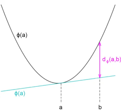
Letφ:S_7→Rbe a strictly convex function defined on a convex setS_⊆Rksuch thatφis differentiable on the relative interior ofS,ri(S). TheBregman divergence, orBregman loss functions (BLFs),d_φ:ri(S)×S7→[0,∞) is defined as

d_φ(a,b)=φ(b)−φ(a)−­b₋a,∇φ(a)®

(13) where∇φ(a) is a gradiant ofφin pointaand angle brackets〈〉is notation for dot product [Bregman, 1967] [Banerjee et al., 2005]. In Figure 10, there is graphical representation of Bregman divergence.

Log Loss as Divergence It is called Kullback-Leiber (KL) divergence when used as a divergence measure, andlogarithmic loss (log loss)when used as a loss measure [Kullback and Leibler, 1951]:

d_LL(a,b)= d X i=1 b_ilogbi a_i

Brier Score as Divergence It is calledsquared Euclidean distancewhen used as a divergence measure, andmean squared errororBrier score when used as a loss measure. d_BS(a,b)= ||a₋b_||2₌ d X i=1 (a_i−b_i)2 Graphical representation of Euclidean distance is in Figure 12.

Figure 9. Convex function.

Figure 10. Visual representation of Bregman divergence. Divergence d_φ(a,b) is the difference between∇φ(a) in point bandφ(b).

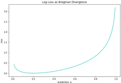
Figure 11. Log-loss as Bregman divergence, withb=0.2.

4

Derivation of Proper Scoring Rules

4.1

Brier Score

In this section, we will find and prove the relation between Brier score and additive cost context. This section mostly follows [Hernández-Orallo et al., 2012].

As it was discussed earlier, c₀stands for cost of false negative and c₁is cost of false positive. Further, cost magnitudebis equal tob₌c₀₊c₁. Cost magnitude will be scaled to 2 to ensure commensurability with error rate,b=2. Let us suppose thatc₀has uniform distribution in [0; 2], thenc₁₌2−c₀. To make notation simpler, a new variableswill be introduced that has uniform distribution over [0, 1]. Then,

c₀=2s andc₁=2−c₀=2−2s=2(1−s). This cost context will be calledadditive. According to the definitions in Section 2, expected proportion of false positives at thresholdsisπ0(1−F0(s)), and expected proportion of false negative at threshold

s isπ1F1(s).

To calculate cost of false negatives, one would multiply cost of one false negative (2s) by number of false negativesπ0(1−F0(s)). Similarly, cost of false positives is

multiplication of 2(1−s) andπ1F1(s). Clearly, the total cost at thresholdsdenoted

byLis sum of false negative and false positive costs.

By default, integral has limits [0;+∞] and range ofsis shown by p.d.f is shown by p.d.f. w(s). Function w(s) is equal to 1 only if 0≤s≤1. Then total cost L at threshold sis: L₌ Z ∞ 0 h 2sπ₀(1−F₀(s))+2(1−s)π1F1(s) i w(s)ds

Sincew(s) is equal to 1 only if 0≤s≤1, integral’s limits will be changed to [0; 1],

w(s) will cancel out because it is always 1 in new limits.

L₌ Z 1 0 h 2sπ₀(1−F₀(s))+2(1−s)π1F1(s) i ds (14)

Theorem 1. Let us assume additive cost context, c₀₊c₁₌2, and probabilistic scores and a decision threshold of probabilistic scores equal tos. Then expected loss L under a uniform distribution of s is equal to expected Brier Score.

Proof. Expected Brier score for actual class 1 will be denoted asBS₁. Assuming

s is the predicted probability of getting class 1, loss of for class 1 will be equal to squared difference between probabilitys and actual class 1. Since value ofsis not known, loss will be integrated overs in range [0; 1], as it is range for all possible values of s. Then, expected Brier score when actual class is 1:

BS1=

Z 1

0

Analogically, Brier score if actual class is 0 will be denoted asBS₀and loss of class 0 will be equal to squared difference betweensand 0 and it will be integrated oversin range [0; 1]. Expected Brier score when actual class is 0:

BS₀₌ Z 1 0 (0−s)2f₀(s)ds₌ Z 1 0 s2f₀(s)ds

Expected loss for both classes will be weighted average of Brier scores for each classes, weighted by proportion of those classesπ0andπ1:

BS₌π₀ Z 1 0 s2f₀(s)ds₊π₁ Z 1 0 (1−s)2f₁(s)ds (15) Next step we will take expected loss for additive context from Eq.(14) and break it into 2 separate integrals:

L₌ Z 1 0 h 2sπ₀(1−F₀(s))+2(1−s)π1F1(s) i ds =π0 Z 1 0 2s(1−F0(s))ds+π1 Z 1 0 2(1−s)F1(s)ds (16)

Clearly, first integral is expected loss when actual class is 0 and second integral is expected loss when actual class is 1.

L₌π₀L₀₊π₁L₁ L₀₌ Z 1 0 2s(1−F₀(s))ds L₁₌ Z 1 0 2(1−s)F₁(s)ds (17)

Now let us integrate the expected losses using integration by parts, where

u=(1−F₀(s)) anddv=2sds, then du= −f₀(s)dsandv=s2:

L₀₌ Z 1 0 2s³1−F₀(s)´ds₌s2³1−F₀(s)´¯¯ ¯ 1 s=0+ Z 1 0 s2f₀(s)ds (18) SinceF₀(0)=0 andF₀(1)=1 : s2³1−F₀(s)´¯¯ ¯ 1 s=0=1 2³₁ −F₀(1)´−02³1−F₀(0)´=1(1−1)−0=0 Then expected loss for class 0:

L0=s2 ³ 1−F0(s) ´¯ ¯ ¯ 1 s=0+ Z 1 0 s2f0(s)ds= Z 1 0 s2f0(s)ds (19)

Expected loss for class 1, using integration by parts, where u₌F₁(s) and dv₌ 2(1−s)ds, thendu=f₁(s)dsandv= −(1−s)2: L₁₌ Z 1 0 2(1−s)F₁(s)ds_{= −}(1−s)2F₁(s) ¯ ¯ ¯ 1 s=0+ Z 1 0 (1−s)2f₁(s)ds (20) SinceF₁(0)=0: (1−s)2F1(s) ¯ ¯ ¯ 1 s=0=(1−1) 2_F 1(1)−(1−0)2F1(0)=02·1−12·0=0

Then expected loss for class 1:

L₁₌(1−s)2F₁(s) ¯ ¯ ¯ 1 s=0+ Z 1 0 (1−s)2f₁(s)ds₌ Z 1 0 (1−s)2f₁(s)ds (21) Expected loss for both classes, following Eq. (17):

L₌π₀ Z 1 0 s2f₀(s)ds₊π₁ Z 1 0 (1−s)2f₁(s)ds

Which is equal to Brier score in Eq. (15). Thus, it is proven that Brier score is equal to expected loss under additive cost context, probabilistic scores and a decision threshold equal tos.

■

Brier score is proper for any number of classes; below is the proof of Brier score’s properness for binary classification.

Theorem 2. Assuming binary classification, Brier score is proper.

Proof. In binary classification, y has two possible values, Y ₌{0, 1}. If y₌1, expected Brier score is:

BS₁₌(y₋s)2=(1−s)2 And if y₌0, expected Brier score is:

BS₀₌(y₋s)2=(0−s)2=s2

Brier score is proper if for anyqit is minimized ats=q. One can take derivative of Brier Score show that derivative is equal to 0 if and only ifs₌q. Then:

q³(1−s)2´0+(1−q)³(s2)´0=0

−2q(1−s)+(1−q)2s₌0

−q₊qs₊s₋qs₌0

q₌s

(22)

Figure 13. Restrictions toc₀and c₁for Inverse score.

4.2

Inverse Score

In the previous section, costsc₀,c₁both had uniform distribution but were perfectly anti-correlated. Let us now introduce a new cost context, where bothc₀,c₁will have independent uniform distributions. This cost context will be calledindependent uniform. A new score will be introduced, based on independent uniform cost context.

At first, a special case will be introduced, where distributions of c₀,c₁will be over [0; 1]. These distributions are displayed in Figure 13.

Assuming calibrated threshold, t₌ c0

c0+c1. At thresholdt proportions of false

positives and false negatives are denoted by 1−F₀(t) andF₁(t), respectively. Then expected loss is equal to:

L₌ Z ∞ 0 Z ∞ 0 · c₀π₀³1−F₀³ c0 c0+c1 ´ +c₁π₁F₁³ c0 c0+c1 ´¸ w(c₀,c₁)d c₀d c₁ (23) where p.d.f. w(c₀,c₁) in special case is equal to 1 when c₀ and c₁ fall into their defined distributions, that is 0≤c_0≤1 and 0≤c_1≤1, and w(c₀,c₁) is equal to 0 otherwise.

Expected Inverse Score can be calculated as:

I S₀₌ ( _2p−1 6(p−1)2+ 1 6 if p∈[0; 1 2] −_3p1 +5₆ if p_∈(1₂; 1] I S₁₌ ( ₁ 3(p−1)+ 5 6 if p∈[0; 1 2] 1−2p 6p2 + 1 6 if p∈( 1 2; 1] (24)

where pis estimated probability of predicting class 1.

Theorem 3. Let us assume independent uniform cost context, c₀,c₁have uniform distributions in[0; 1], and probabilistic scores and a decision threshold equal to s₌ c0

c0+c1. Then expected lossL under a uniform distribution of c0and c1is equal to

expected Inverse score. Proof. Inverse score:

I S₌1 3 · Z 1₂ 0 ³ 2s−1 2(s₋1)2+ 1 2 ´ f₀(s)ds₊ Z 1 1 2 ³ −1 s+ 5 2 ´ f₀(s)ds + Z 1₂ 0 ³ 1 s₋1+ 5 2 ´ f₁(s)ds₊ Z 1 1 2 ³1−2s 2s2 + 1 2 ´ f₁(s)ds ¸

In expected loss from Eq. (23), substitutions₌ c0

c0+c1 can be made. Then,c0=

sc1 1−s and d c0 = ³ sc1 (1−s) ´0 ds= c1

[0;+∞], s is in rangeh₀₊0_c

1;

+∞ +∞+c1

i

, which is equal to s_∈[0; 1]. New integration is now overs in range [0; 1] and overc₁ in range [0;+∞]:

L₌ Z ∞ 0 Z 1 0 · _sc 1 1−s ³ 1−F₀(s)´+c₁F₁(s) ¸ w³ sc1 1−s,c1 ´ c₁ (1−s)2dsd c1 (25) Then, w¡sc₁ 1−s,c1 ¢

will be equal to 1 in two cases: 1. s_∈¡ 0;1₂¢ ,c_1∈¡ 0; 1¢ , because sc1 1−s<1⇒sc1<1−s⇒s< 1 c1+1 2. s∈¡1₂; 1¢,c1∈ ¡ 0;1−_ss¢, because sc1 1−s<1⇒ s 1−sc1<1⇒c1< 1−s s

With new restrictions to sand c₁, Eq. (25) could be represented as the sum of four following integrals:

L= Z 1₂ 0 Z 1 0 sc1 1−s c1 (1−s)2 ³ 1−F₀(s)´d c₁ds + Z 1 1 2 Z (1−s)/s 0 sc₁ 1−s c₁ (1−s)2 ³ 1−F₀(s)´d c₁ds + Z 1₂ 0 Z 1 0 c2₁ (1−s)2F1(s)d c1ds + Z 1 1 2 Z (1−s)/s 0 c2₁ (1−s)2F1(s)d c1ds (26)

Let us solve these 4 integrals separately.

Integration of 1st integral Integration over c₁: Z 1 0 sc1 1−s c1 (1−s)2 ³ 1−F0(s) ´ d c1= ³ 1−F0(s) ´ s (1−s)3 Z 1 0 c2₁d c1= ³ 1−F0(s) ´ s (1−s)3 1 3 Integration by parts over s, where u=1−F0(s) and dv= ₍₁₋s_s)3ds, then du=

−f0(s)dsandv=_2(s2s₋−₁₎12: 1 3 Z 1 2 0 s (1−s)3 ³ 1−F0(s) ´ ds=1 3 ·₁ 2− 1 2F0(0)+ Z 1 2 0 2s₋1 2(s₋1)2f0(s)ds ¸ (27)

Integration of 2nd integral Integration over c₁: Z (1−s)/s 0 sc₁ 1−s c₁ (1−s)2 ³ 1−F₀(s)´d c₁₌³1−F₀(s)´ s (1−s)3 Z (1−s)/s 0 c2₁d c₁₌³1−F₀(s)´ 1 3s2

Integration by parts overs, whereu₌1−F₀(s) anddv₌ 1 s2ds, thendu= −f0(s)ds andv_{= −}1_s: 1 3 Z 1 1 2 1 s2 ³ 1−F₀(s)´ds₌1 3 · 2−2F₀(1 2)−1+F0(1) Z 1 1 2 ³ −1 s ´ f₀(s)ds ¸ (28)

Integration of 3rd integral Integration over c₁: Z 1 0 c₁ (1−s)2c1F1(s)d c1=F1(s) 1 (1−s)2 Z 1 0 c2₁d c₁₌F₁(s) 1 (1−s)2 1 3 Integration by parts over s, whereu₌F₁(s) and dv₌ 1

(1−s)2ds, thendu=f1(s)ds andv₌₁1 −s: 1 3 Z 1₂ 0 1 (1−s)2F1(s)ds= 1 3 · 2F₁³1 2 ´ −F₁(0)+ Z 1₂ 0 1 s₋1f1(s)ds ¸ (29)

Integration of 4th integral Integration over c₁: Z (1−s)/s 0 c₁ (1−s)2c1F1(s)d c1=F1(s) 1 (1−s)2 Z (1−s)/s 0 c2₁d c₁₌F₁(s)1−s 3s3

Integration by parts overs, whereu₌F₁(s) anddv₌1−s

s3 ds, then du=f1(s)dsand v₌2s−1 2s2 : 1 3 Z 1 1 2 1−s s3 F1(s)ds= 1 3 · 1 2F1(1)+ Z 1 1 2 1−2s 2s2 f1(s)ds ¸ (30) Sum of results of integrals in Eq. (27 – 30) is equal to:

L₌1 3 · 1 2− 1 2F0 ³ 0´−1+F₀³1´+2−2F₀³1 2 ´ +2F₁³1 2 ´ −F₁³0´+1 2F1 ³ 1´ + Z 1₂ 0 f₀(s)³ 2s−1 2(s₋1)2 ´ ds₊ Z 1 1 2 f₀(s)³−1 s ´ ds + Z 1₂ 0 f₁(s)³ 1 s₋1 ´ ds₊ Z 1 1 2 f₁(s)³1−2s 2s2 ´ ds ¸ (31)

Some transformations need to be done, for i₌0, 1:

F_i¡ 0¢

=0, F_i¡ 1¢

Expected loss after transformations: L₌1 3 · 1 2−0−1+1+2−2F0 ³1 2 ´ +2F₁³1 2 ´ −0+1 2 + Z 1₂ 0 f₀(s)³ 2s−1 2(s−1)2 ´ ds₊ Z 1 1 2 f₀(s)³−1 s ´ ds₊ Z 1₂ 0 f₁(s)³ 1 s−1 ´ ds₊ Z 1 1 2 f₁(s)³1−2s 2s2 ´ ds ¸ =1 3 · 3−2F₀³1 2 ´ +2F₁³1 2 ´ − + Z 1 2 0 f0(s) ³ 2s−1 2(s₋1)2 ´ ds+ Z 1 1 2 f0(s) ³ −1 s ´ ds+ Z 1 2 0 f1(s) ³ 1 s₋1 ´ ds+ Z 1 1 2 f1(s) ³1−2s 2s2 ´ ds ¸ Transformations for 2F₀³1 2 ´ and 2F₁³1 2 ´ : 2F₁³1 2 ´ =2 Z 1₂ 0 f₁(s)ds₌ Z 1₂ 0 f₁(s)ds₊1− Z 1 1 2 f₁(s)ds −2F₀³1 2 ´ = −2 Z 1₂ 0 f₀(s)ds_{= −} Z 1₂ 0 f₀(s)ds₋1+ Z 1 1 2 f₀(s)ds

Which means that−1 will be added to coefficients ofR1₂

0 f0(s)dsand

R1

1 2

f₁(s)ds, and 1 will be added to the other two coefficients. Expected loss after transformations:

L₌1 3 · 3+ Z 1₂ 0 f₀(s)³ 2s−1 2(s₋1)2−1 ´ ds₊ Z 1 1 2 f₀(s)³−1 s+1 ´ ds + Z 1₂ 0 f₁(s)³ 1 s₋1+1 ´ ds₊ Z 1 1 2 f₁(s)³1−2s 2s2 −1 ´ ds ¸ Transformations for 3: 3=3 2+ 3 2= 3 2 hZ 1 2 0 f₀(s)ds₊ Z 1 1 2 f₀(s)dsi₊3 2 hZ 1 2 0 f₁(s)ds₊ Z 1 1 2 f₁(s)dsi =3 2 hZ 1 2 0 f₀(s)ds₊ Z 1 1 2 f₀(s)ds₊ Z 1₂ 0 f₁(s)ds₊ Z 1 1 2 f₁(s)dsi

Which means that to all coefficients under integral 3₂ will be added. Final form after transformations:

L₌1 3 · Z 1₂ 0 f₀(s)³ 2s−1 2(s−1)2+ 1 2 ´ ds₊ Z 1 1 2 f₀(s)³−1 s+ 5 2 ´ ds + Z 1₂ 0 f₁(s)³ 1 s₋1+ 5 2 ´ ds₊ Z 1 1 2 f₁(s)³1−2s 2s2 + 1 2 ´ ds ¸ (32) ■

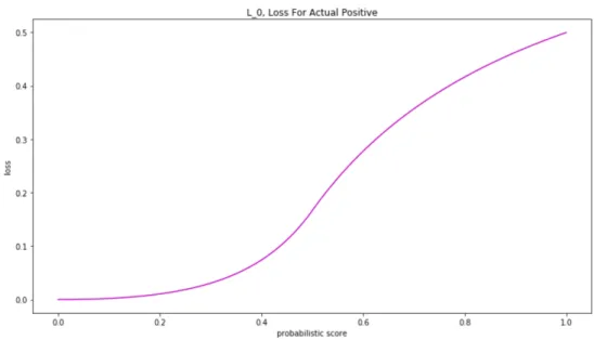
If we take coefficients of f₀(s) from Eq. (32), we get loss functionL₀ for actual positive label (0) that depends on probabilistic scores, and coefficients of f₁(s) makes loss function L1 for actual negative label (1) in the same way. Eq. (33)

highlights final loss, functions in Figures 15 and 16 display their plots.

L0= ( _2s−1 6(s−1)2 +1₆ ifs∈[0;1₂] −_3s1 +5₆ ifs∈(1₂; 1] L₁₌ ( ₁ 3(s−1)+ 5 6 ifs∈[0; 1 2] 1−2s 6s2 +1₆ ifs∈(1₂; 1] (33)

Theorem 4. Inverse Score is proper.

Proof. Similarly to Theorem (2) about Brier score’s properness, Inverse Score is proper if for any q, it is minimized at s=q. One can take derivative of Inverse Score show that derivative is equal to 0 if and only ifs₌q. Then:

If s_∈[0;1₂]: q³ 1 s₋1 ´0 +(1−q)³ 2s−1 2(s₋1)2 ´0 =0 q³₋ 1 (1−s)2 ´ +(1−q)³ s (1−s)3 ´ =0 −q(1−s)+(1−q)s₌0 s=q (34) If s_∈(1₂; 1]: q³1−2s 2s2 ´0 +(1−q)³−1 s ´0 =0 q³s−1 s3 ´ +(1−q)³1 s2 ´ =0 q(s₋1)+(1−q)s₌0 s₌q (35)

Figure 15. Plot ofL₀, loss when actual class is positive, with respect to probabilistic score

Figure 16. Plot ofL1, loss when actual class is negative, with respect to probabilistic

When score is minimal,q₌s. Thus, Inverse Score is proper. ■

4.3

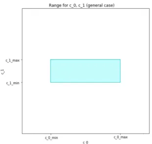
Possible Generalization of Inverse Score

In general case, c₀has uniform distribution in [c_0min,c_0max] andc₁ has uniform distribution in (c_1min,c_1max]. These distributions are displayed in Figure 14.

Let a=c_0min,b=c_0max,d=c_0min, e=c_1maxfor the easiness to comprehend. Then, following the formula in Eq. (25) on page 33,w¡sc₁

1−s,c1 ¢ will be equal to 1 in two cases: 1. s∈¡ _e a+e; b b+e ¢ ,c1∈¡d;e¢ 2. s∈¡ _b b+e; b b+d ¢ , c₁∈¡ d;b1−_ss¢

Then the integral from Eq. (25) can be broken down to the sum of 4 integrals:

L₌ Z b/(b+e) a/(a+e) Z e d sc₁ 1−s c₁ (1−s)2 ³ 1−F₀(s)´d c₁ds + Z b/(d+b) b/(b+e) Z b(1−s)/s d sc₁ 1−s c₁ (1−s)2 ³ 1−F₀(s)´d c₁ds + Z b/(b+e) a/(a+e) Z e d c₁ (1−s)2F1(s)d c1ds + Z b/(d+b) b/(b+e) Z b(1−s)/s d c₁ (1−s)2F1(s)d c1ds (36)

Solving this integral would result in a family of proper scoring rules. This part remains to be done in the future work.

5

Experiments

In Section 4 Theorem 3 was proven, which states that for probabilistic scores, independent cost contexts and a threshold equal tos₌ c0

c0+c1, expected loss under a

uniform distribution of c₀and c₁is equal to Inverse Score. In this section, it will be shown on the experiments.

5.1

Setup

The experiments began by creating toy dataset with 5,000 instances. Binary classification was used and dataset was balanced, labels {0, 1}were assigned to instances randomly with probability 0.5. Scores of instances with label 1 had distribution N(−µ, 1) and scores of instances with label 0 had distribution N(µ, 1). From scores, probabilistic scores were calculated using formula p₌ 1

1+e−2s.

Cost Calculations To calculate total cost, independent cost context was used, which was introduced in Section 4.2. It means that false negative cost c₀and false positive costc₁both have uniform distributions and do not depend on the values of each other. Thresholdsfor classification is s₌ c0

c0+c1. So, instance will be predicted

negative if its probabilistic score p_>sand positive otherwise.

In this case, distributions will be the same and equal to [0; 1]. 5,000 iterations were made; in each iteration, number of false positivesF P and proportion of false negatives F N were calculated. T otal is the number of all instances.For each iteration, cost was equal to:

C=F P·c0+F N·c1

T otal

To estimate expected total cost, costsCfrom all iterations were averaged.

Loss Calculations To calculate loss, loss function in Eq. (33) from page 36 was used:

If instance is actually of positive class:

L₀₌ ( _2p−1 6(p−1)2+ 1 6 if p∈[0; 1 2] −_3p1 +5₆ if p_∈(1₂; 1]

If instance is actually of negative class:

L₁₌ ( ₁ 3(p−1)+ 5 6 if p∈[0; 1 2] 1−2p 6p2 + 1 6 if p∈( 1 2; 1]

5.2

Results

In Figure 17, total cost and expected loss are compared using different µ. As expected, expected loss generalized total cost very well with little to no bias, where pink line describes expected loss calculated from the experiments, and green line represents total cost. Loss and cost both decrease with growth of µ, because instances of different classes are separated further and it is harder to predict them incorrectly. It is possible to reduce bias further by increasing the number of iterations when calculating total cost.

6

Conclusion

Classification is a fundamental task in supervised machine learning with an extremely wide range of applications. In case of cost-sensitive learning, evaluation of classifier performance becomes non-trivial due to operating conditions and cost contexts, which span ranges of cost values.

It has been previously shown that classifier evaluation under well-known operating conditions are handled with appropriate proper scoring rules.

In this thesis, a new operating condition for binary classification with uniformly distributed costsc₀and c₁ was introduced, along with a corresponding new proper scoring rule. Its applicability and properness was proven theoretically and con-firmed experimentally. The proof was performed for a special case of cost context with fixed distributions, where both costs had distributions [0; 1].

Following the proof, new proper scoring rule can be used when cost context involves independent uniform distributions for both costs.

The future work may involve complete the proof for general case of distributions, which would result in a family of proper scoring rules.

References

[Banerjee et al., 2005] Banerjee, A., Guo, X., and Wang, H. (2005). On the opti-mality of conditional expectation as a Bregman predictor. IEEE Transactions of Information Theory.

[Boyd and Vandenberghe, 2004] Boyd, S. and Vandenberghe, L. (2004). Convex Optimization. Cambridge University Press, 7 edition.

[Bregman, 1967] Bregman, L. M. (1967). A relaxation method of finding the common point of convex sets and its application to the solution of problems in convex programming.Journal of Computational Mathematics and Mathematical Physics.

[Brier, 1950] Brier, G. W. (1950). Verification of forecasts expressed in terms of probability. Monthly Weather Review.

[Brownlee, 2018] Brownlee, J. (2018). A gentle introduction to probabil-ity scoring methods in python. https://machinelearningmastery.com/

how-to-score-probability-predictions-in-python/.

[Buja et al., 2005] Buja, A., Stuetzle, W., and Shen, Y. (2005). Loss func-tions for binary class probability estimation and classification: Struc-ture and applications. http://www-stat.wharton.upenn.edu/~buja/PAPERS/

paper-proper-scoring.pdf.

[Elkan, 2001] Elkan, C. (2001). The foundations of cost-sensitive learning. Proceed-ings of the Seventeenth International Joint Conference on Artificial Intelligence. [Fawcett, 2005] Fawcett, T. (2005). An introduction to ROC analysis. Pattern

Recognition Letters.

[Fawcett, 2015] Fawcett, T. (2015). The Basics of Classifier Evaluation: Part 1.

https://www.svds.com/the-basics-of-classifier-evaluation-part-1/.

[Flach, 2015] Flach, P. A. (2015). Cost-sensitive classification meets proper scoring rules.http://dmip.webs.upv.es/LMCE2015/Papers/LMCE_2015_submission_5.

pdf.

[Garthwaite et al., 2005] Garthwaite, P. H., Kadane, J. B., and O’Hagan, A. (2005). Statistical methods for eliciting probability distributions. Journal of the Ameri-can Statistical Association.

[Gneiting and Raftery, 2007] Gneiting, T. and Raftery, A. E. (2007). Strictly Proper Scoring Rules, Prediction, and Estimation. Journal of the American Statistical Association.

[Good, 1952] Good, I. J. (1952). Rational decisions. Journal of the Royal Statistical Society. Series B (Methodological).

[Hand, 2009] Hand, D. J. (2009). Measuring classifier performance: a coherent alternative to the area under the ROC curve. Springer Science+Business Media. [Hernández-Orallo et al., 2011] Hernández-Orallo, J., Flach, P. A., and Ferri, C. (2011). Brier Curves: A New Cost-Based Visualisation of Classifier Performance.

International Conference on Machine Learning.

[Hernández-Orallo et al., 2012] Hernández-Orallo, J., Flach, P. A., and Ferri, C. (2012). A Unified View of Performance Metrics: Translating Threshold Choice into Expected Classification Loss. Journal of Machine Learning Research. [Kull and Flach, 2015] Kull, M. and Flach, P. A. (2015). Novel decompositions

of proper scoring rules for classification: Score adjustment as precursor to calibration. Joint European Conference on Machine Learning and Knowledge Discovery in Databases.

[Kullback and Leibler, 1951] Kullback, S. and Leibler, R. A. (1951). On informa-tion and sufficiency. The annals of mathematical statistics.

[Murphy and Winkler, 1970] Murphy, A. H. and Winkler, R. L. (1970). Scoring rules in probability assessment and evaluation. Acta Psychologica.

[Powers, 2011] Powers, D. M. W. (2011). Evaluation: from precision, recall and f-measure to ROC, informedness, markedness & correlation. Journal of Machine Learning Technologies.

[Santos-Rodríguez et al., 2009] Santos-Rodríguez, R., Guerrero-Curieses, A., Alaiz-Rodríguez, R., and Cid-Sueir, J. (2009). Cost-sensitive learning based on bregman divergences. Springer Science+Business Media.

[Sun et al., 2011] Sun, Y., Wong, A., and Kamel, M. S. (2011). Classification of imbalanced data: a review. International Journal of Pattern Recognition and Artificial Intelligence.

[Tharwat, 2018] Tharwat, A. (2018). Classification assessment methods. Applied Computing and Informatics.

[Volovich, 2019] Volovich, K. (2019). What’s a Good Clickthrough Rate? New Benchmark Data for Google AdWords. https://blog.hubspot.com/agency/

google-adwords-benchmark-data.

[Winkler and Murphy, 1968] Winkler, R. L. and Murphy, A. H. (1968). ‘Good’ Probability Assessors. Journal of Applied Meteorology and Climatology.

[Wolpert, 1996] Wolpert, D. H. (1996). The lack of a priori distinctions between learning algorithms. Neural Computation.

[Yao, 2017] Yao, M. (2017). Chihuahua or muffin? My search for the best computer vision API. https://medium.freecodecamp.org/

Appendix

I. Code

Source code for this thesis is located in the following GitHub repository:

https://github.com/sherlie/inverse-score

II. Licence

Non-exclusive licence to reproduce thesis and make thesis

public

I,Diana Grygorian,

1. herewith grant the University of Tartu a free permit (non-exclusive licence) to reproduce, for the purpose of preservation, including for adding to the DSpace digital archives until the expiry of the term of copyright,

Classifier Evaluation With Proper Scoring Rules supervised by Meelis Kull

2. I grant the University of Tartu a permit to make the work specified in p. 1 available to the public via the web environment of the University of Tartu, including via the DSpace digital archives, under the Creative Commons licence CC BY NC ND 3.0, which allows, by giving appropriate credit to the author, to reproduce, distribute the work and communicate it to the public, and prohibits the creation of derivative works and any commercial use of the work until the expiry of the term of copyright.

3. I am aware of the fact that the author retains the rights specified in p. 1 and 2.

4. I certify that granting the non-exclusive licence does not infringe other persons’ intellectual property rights or rights arising from the personal data protection legislation.

Diana Grygorian 16.05.2019