The role of graphlets in viral processes on networks
Samira Khorshidi
∗Mohammad Al Hasan
†George Mohler
‡Martin Short
§Abstract
Predicting the evolution of viral processes on networks is an important problem with appli-cations arising in biology, the social sciences, and the study of the Internet. In existing works, mean-field analysis based upon degree distribution is used for the prediction of viral spread-ing across networks of different types. However, it has been shown that degree distribution alone fails to predict the behavior of viruses on some real-world networks and recent attempts have been made to use assortativity to address this shortcoming. In this paper we show that assortativity also fails to adequately predict the spread of viruses for a number of real-world networks. We propose using the graphlet frequency distribution in combination with assortativ-ity to explain variations in the evolution of viral processes across networks with identical degree distribution. Using a data driven approach, by coupling predictive modeling with viral process simulation on real-world networks, we show that simple regression models based on graphlet frequency distribution can explain over 95% of the variance in virality on networks with the same degree distribution but different network topologies. Our results not only highlight the importance of graphlets but also identify a small collection of graphlets which may have the highest influence over the viral processes on a network.
1
Introduction
A variety of dynamic phenomena, including Youtube video views [7], Tweet resharing [32], viral marketing campaigns [17], the spread of computer viruses on the Internet [2], and gang retaliation [30] can be explained as evolving viral processes on networks. As such, the study of the evolution of viral processes on networks has attracted considerable attention in recent years. It is now well known that for a connected network, the largest eigenvalue of its adjacency matrix is a good metric for predicting the viral process in that network [5,12,16]. The largest eigenvalue can be roughly estimated by the average degree of the network [18], but the complete degree distribution of the network is more expressive than the point estimate of average degree, and has therefore also been considered for predicting these viral processes. A common approach along these lines is to employ a mean-field analysis where independence assumptions on the nodes are used [1, 4, 6, 9, 10]. More recently it has been shown that in some cases, including real-world networks, these mean-field assumptions fail to predict the viral spreading [13]. Consequently, assortativity has been proposed for addressing the limitations of the degree-based, mean-field analyses [15,31], and through degree-preserving network rewiring procedures, it has been shown that the spectral radius of a graph can exhibit great fluctuations across networks with the same degree distribution and that assortativity can be used to explain this variation. While there is a clear correlation between assortativity and the dynamics of viral processes on graphs, the fact remains that, if we control for both assortativity and degree distribution, viral diffusions on networks with differing topologies can still exhibit greatly different behaviors.
∗Computer and Information Science, Indiana University - Purdue University Indianapolis, [email protected] †Computer and Information Science, Indiana University - Purdue University Indianapolis, [email protected] ‡Computer and Information Science, Indiana University - Purdue University Indianapolis, [email protected] §School of Mathematics, Georgia Institute of Technology, [email protected]
___________________________________________________________________ This is the author's manuscript of the article published in final edited form as:
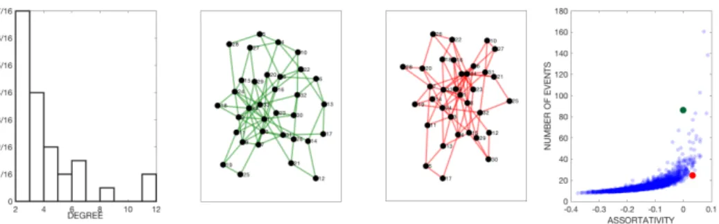
We illustrate this observation with the following example. In Figure 1, we display results for a Hawkes process [7] simulation on 2500 networks with identical degree distribution sampled via degree preserving rewiring [22] from the Karate network [28]. In the Hawkes branching process model, an initial event occurs at a randomly chosen node and then subsequent generations of events occur at neighboring nodes of previous events with a fixed probability. In Figure 1, we plot assorativity vs. the expected total number of events (at time infinity) of the Hawkes process for each of the simulated networks. While assortativity partially explains the behavior of the process, for the two highlighted networks with identical degree distribution and similar assorta-tivity, the expected total number of events in the process differs by a factor of 4. So, we need to extend our analysis beyond degree distribution and assortativity for better understanding of the dynamics of a viral process over a network.
Figure 1: Hawkes process simulation on 2500 rewired Karate networks. Degree distribution (far left) is fixed for all of the 2500 networks. The Expected number of events in a cascade vs assortativity (far right). Two example networks (middle) corresponding to large differences in virality despite similar assortativity and identical degree distribution.
In this paper we propose using the frequency distribution of graphlets (see Figure 3 for a preview) to explain the variation in viral processes observed in Figure 1. Specifically, we show that graphlet frequencies are good predictors for explaining the variation of the evolution of viral processes over a collection of networks for which the degree distribution is kept fixed. Our results not only highlight the importance of graphlets but also identify a small collection of graphlets that may have the highest influence over the viral processes on a network.
The rest of the document is organized as follows. In Section 2, we discuss some back-ground materials, including graphlets and viral process models. In Section 3, we discuss the methodologies of our proposed analysis. In Section 4 we present our results on five real-world networks illustrating the role of graphlets in viral processes. In the final section, we discuss the implications of these results and directions for future research.
2
Background
In this paper, we will be making several different measurements reflecting the topology of net-works – from degree distribution to assortativity to graphlet distribution – as well as simulating two different viral processes – the Hawkes process and Susceptible-Infected-Susceptible model – on networks. We provide some background materials on these topics in this section.
2.1
Degree Distribution
Thedegreeof a node is the number of connections of that node to other nodes in the network. The degree distribution is a discrete probability distribution of degrees over the nodes in the network. Directed networks have two different degree distributions, the in-degree and the out-degree distributions. In this study, we restrict our attention to undirected networks for which only one degree distribution is defined.
Figure 2: The left figure shows a graph with positive assortativity where nodes with high degree are connected to other nodes with high degree (assortativity= 5.4). The right graph is an example of a disassortative network,(assortativity=−0.88) where the hubs connect to low degree nodes.
g1 g2 3-node graphlets g3 g4 g5 g6 g7 g8 4-node graphlets 5-node graphlets g9 g10 g11 g12 g13 g14 g15 g16 g17 g18 g19 g20 g21 g22 g23 g24 g25 g26 g27 g28 g29
Figure 3: Undirected graphlets with 3, 4, and 5 vertices.
2.2
Assortativity
Assortativity, or assortative mixing, is defined by the tendency of a network’s nodes to be connected to others nodes that are similar in some way. While there are several different mathematical definitions, we will refer to assortativity as the Pearson correlation coefficient of degrees at either ends of a network edge [21]. In this case the assortativity is given by the formula [21], A= M −1P ijiki−[M −1P i 1 2(ji+ki)] 2 M−1P i 1 2(j 2 i +ki2)−[M−1 P i 1 2(ji+ki)]2 , (1)
where the edges in a network are indexed byi= 1, ..., M andji, kiare the degrees of the nodes at the ends of edgei. In Figure 2, we provide examples of two social networks from the Network Repository [28] with different assortativity, one positive and one negative.
2.3
Graphlets
Graphletscan be defined as small, connected1, non-isomorphic, induced subgraphs of a large network. In this study, we work with all possible graphlets having k∈ {3,4,5}vertices. If the graphlet edges are undirected, there are 29 such graphlets as shown in Figure 3. We refer to a graphlet with k vertices as a k-Graphlet; note that a 1-Graphlet is simply a vertex and a 2-Graphletis simply an edge. The frequency of a graphletgiin a graphGis the total number of distinct embeddings of that graphlet gi in the graph G. Graphlet frequency distribution (GFD) is the normalized frequency of the graphlets. As real life networks are generally sparse, frequencies of larger sized graphlets shrink exponentially, so in GFD, we use a logarithm scale
1disconnected graphlets have also been considered in several graphlet based works, but in this work we only consider connected graphlets because connectedness is essential for the evolution of a viral process on a network.
for comparing various frequencies so that the number of occurrences of larger-sized graphlets against that of the smaller-sized ones are scaled appropriately.
The frequency distribution of graphlets in a network captures the local topology around the vertices of the network and it has a number of uses in network analysis and prediction. For example, the frequencies of various graphlets can be used for building a global fingerprint for a network such that the fingerprints of different networks arising from a real-life domain are almost identical [25]. Transition of graphlets over temporal snapshots of a network has also been shown to improve link prediction models for dynamic networks [23].
A key challenge for finding graphlet frequency distribution is the high computational cost of graphlet enumeration or counting. However, in recent years, several efficient algorithms have become available that generate exact graphlet counting [24, 25]. Yet, for very large networks exact counting of graphlets is not feasible. So, there exist methods (such as, GUISE and its variants [3, 26, 27]), which can generate approximate graphlet frequency distributions through uniform sampling of graphlets. Sampling based methods provide very good approximations of graphlet frequency distributions and can scale to graphs with millions of vertices. In this work, we use GUISE algorithm for computing the graphlet frequency distributions of a network.
2.4
Hawkes process model
The Hawkes process is a specific kind of self-exciting point process whereby discrete events occur according to a stochastic intensityλ(t) that increases in response to events themselves. For a Hawkes process on a network G, given the event observation dyads (ti, vi), whereti is a time value for an event andviis a vertex on which the event occurred, the conditional intensity (rate) of events at nodev,λv(t), is given by the equation
λv(t) =µ+ X t>ti vi∈N(v)
θf(t−ti). (2)
In Equation 2, N(v) is the set of nodes that are neighbor of v onG(note thatv ∈N(v) for this process) so that the intensity is a superposition of a Poisson background intensity µand Poisson intensitiesθf(t−ti) centered at previous event timestisuch that vi is a neighbor ofv on the graphG. The triggering kernelf(t) is a probability density defined on [0,∞) and, when the model is interpreted as a branching process, the productivity parameter θ determines the expected number of direct offspring events at nodevtriggered by an event at a nodevi∈N(v).
2.5
Susceptible-Infected-Susceptible model
The second model we consider is based on the well-known Susceptible-Infected-Susceptible (SIS) model in epidemiology. In this model, each node of the network can be in one of two states at any given time - susceptible or infected. Let S(t) be the set of all susceptible nodes at time t,I(t) be the set of all infected nodes at timet,λv(t) be the rate at which a susceptible node v ∈ S(t) becomes infected, and µu be the rate at which an infected node u ∈ I(t) becomes susceptible. The model is then
λv(t) = X q∈N(v)∪I(t)
θ (3)
µu= 1. (4)
So, a susceptible nodevswitches to being infected via a Poisson process with time varying rate equal to a parameterθ times the number of neighbors ofvthat are infected at that time, and an infected nodeuswitches to being susceptible via a homogeneous Poisson process with rate 1 (without loss of generality). In terms of virality, one may be interested in a scenario in which all nodes are initially susceptible except for a potentially small number of infected, then tracking how many further infections occur as a result of these initial infections. The result will clearly depend on which nodes are initially infected, the adjacency matrix of the newtork A, and the parameterθ.
3
Methologies
Our primary objective is to show that graphlet frequency distribution, in addition to assorta-tivity, is a good predictor for the virality in a network when degree distribution is controlled for. Many earlier works use analytic approaches for finding the influence of network topology or network based metrics on the viral process on a network [5,12]. However, such methods are very cumbersome for graphlets, as graphlets are combinatorially complex objects and their influence over the dynamic process is difficult to represent by a simple model that can be solved analyti-cally. So, in this work we forgo a mathematical analysis in favor of a data science approach to the problem. Our overall strategy is to use simulation and empirical measurement to explore the connection between graphlet distribution and the evolution of viral processes on networks. For this purpose we use several real-world networks as input to a simulation model. Given a particular network and model for a viral process, we perform the following steps:
1. GenerateM synthetic networks through re-wiring (explained below) with identical degree distributions to the original real-world network.
2. For each generated network, compute the assortativity and graphlet frequency distribution. 3. For each generated network, compute the expected number of events,E[N∞], of the viral
process of interest running on the network.
4. RegressE[N∞] against the assortativity and graphlet distribution to assess the role that
graphlets play beyond assortativity and degree distribution. Below we provide more details of the above steps.
3.1
Generating Simulation Graphs
We have shown in the Introduction section, degree distribution and assortativity are not ade-quate for explaining the evolution of a viral process in a network—which motivate us to find the influence of graphlet frequency distribution in a viral process. However, degree distribution does provide a partial explanation of a viral process. To nullify the influence of degree distribution in our analysis, we use degree distribution as a control variable, i.e., we generate a collection of synthetic networks for which degree distribution is a constant.
Generating networks with a given degree distribution is a well-studied problem, specifically for the task of network motif discovery [29]. There are two well-known approaches for solving this problem, (i) edge swapping [14, 19] and (ii) stub-matching. Edge swapping starts from a given graph and makes local modification on the given graph to generate another graph having the same degree sequence. One edge swapping approach that preserves the degree sequence is the following. First, select two edges uniformly at random from the graph G; for example, suppose these aree1 = (a, b) ande2= (c, d). Then, replace these two edges by two new edges
where the second vertices are swapped between the original two edges, assuming those new edges are not already present inG; in our example, these would be the two new edgese3= (a, d) and
e4 = (c, b). If the edgee3 or e4 (or both) already exists in G, this proposed swap is rejected
and the process is repeated with a new pair of randomly chosen edges e1 ande2. It is easy to
see that the degree of each vertex remains invariant under a successful edge swap process. The edge-swapping can be continued and a sequence of graphs can be generated, such that all of these graphs have an identical degree distribution. If we consider the sequence of graphs as a Markov chain, then the stationary distribution of the Markov chain is a uniform distribution over the graphs having identical degree distribution. For stub-matching, the configuration model is very popular [20]. In this method, the algorithm creates as many stubs (dangling half-edges) for each vertex as its degree. Then edges are created by choosing pairs of vertices randomly and connecting their stubs. This approach may create parallel edges, which are dealt with by restarting the process; for large graph the re-starting may become very costly.
In this work, we use the edge-swapping method, as it is easy to implement. By choosing a sufficiently large number of steps for the Markov chain, we generate graphs which are sufficiently different from each other with widely different graphlet frequency distributions.
3.2
Preparing Topology and Virality Data for Regression
For our study, a collection of graphs with identical degree distribution is a regression dataset in which each graph is an instance. For each graph we compute graphlet degree distribution and assortativity, which become the explanatory variables for our regression. Below we discuss how we compute these values for a given graph.
Computing graphlet frequency distribution by counting each of the graphlets in a graph is a costly task as the number of graphlet embeddings grows exponentially with the size of the graphlets. In fact, if both connected and disconnected graphlets are considered, the number of k-graphlets on a graph withKvertices is equal toO( K
k
). In this work, we consider graphlets up to size 5, for which a brute-force graphlet enumeration complexity is equal to (O(K5), which
is not scalable for many real-life networks. An alternative to counting is uniform sampling of graphlet embeddings, which is sufficient to obtain a graphlet frequency distribution. In an earlier work [24], we have shown how graphlets can be sampled under uniform distribution by using a Monte Carlo Markov Chain (MCMC) sampling algorithm. Specifically, we have proposed a method named GUISE, which performs a random walk over the graphlet embeddings by following a double-stochastic transition matrix; the stationary distribution of the Markov chain is a uniform distribution over the graphlet embeddings. By counting the type of graphlets that are traversed in this random walk and then normalizing the vector, GUISE returns a graphlet frequency distribution vector. In this work, we use GUISE algorithm for computing the graphlet frequency distribution. It returns a 29-size vector, in which each component represents the logarithm of the normalized frequency of one of the graphlets in Figure 3. We also compute the assortativity of the network using Eq. 1. The components of the graphlet frequency distribution vector and assortativity (a 30-size vector) become the co-variates of our regression analysis.
The target value of our regression is the expected number of events – excited offspring events in the case of the Hawkes process and secondary infections in the case of the SIS process – that are spawned from a single initiating event placed randomly within the network. The way this target value is computed depends on the viral process used. For the Hawkes process [7, 30, 32], we consider a simplified model where
1. a node is chosen uniformly at random
2. an initial event at timet1= 0 occurs at the chosen node
3. the Hawkes process withµ= 0 is simulated and the total number of events,N∞, at time
infinity is observed
In the case of this simplified model, the expected number of total events is given by, E[N∞] = 1 K1 T·( ∞ X j=1 (θA)j·1), (5)
where K is the number of nodes inG, 1 is a column vector of ones, and A is the adjacency matrix ofG(A is symmetric because the graphGis undirected). The expected total number of eventsE[N∞] will be finite up to a critical threshold value of the productivity parameter,θc.
For the SIS model, we approximate the continuous time version described in Section 2 above with a discrete time version that allows us to more easily count the number of secondary infec-tions arising from a single initially infected node, and which greatly simplifies the simulainfec-tions. Here, time is discretized into units of step 1, and we define a vector I(t) such thatIu(t) = 1 if nodeuis infected at timetand 0 if nodeuis susceptible at timet. Initially,Iu(0) is zero for all uexcept for a single node chosen uniformly randomly. Then the model proceeds via iterations of the following steps:
1. nodes vsusceptible at timetbecome infected at timet+ 1 with probability 1−e−λv(t), whereλv(t) =θ(AI(t))v
2. all nodes infected at timetbecome susceptible at timet+ 1 3. at each timestept >0, the product 1T·
I(t) is equal to the new number of infections 4. the total new infectionsN∞ are observed as time goes to infinity
For this simplified model, an approximation of the expected number of total new infections can be found via E[N∞] = 1 K1 T · K X k=1 ∞ X t=1 I(t;k) (6) Iv(0;k) =δv,k (7) Iv(t+ 1;k) = (1−Iv(t;k))h1−e−θ(AI(t;k))vi . (8)
As in the Hawkes model, the value of E[N∞] is expected to be finite up until some critical
value ofθ, below which the infection is expected to disappear at some finite time (is at most epidemic), and above which the infection in expectation never leaves the network (is endemic).
3.3
Regression Model for Predicting Virality
For each real-world network we simulate M = 500 rewired networks holding the degree dis-tribution fixed. Next, for each simulated network, we compute the assortativity, the graphlet degree distribution, the largest eigenvalueλmax, as well asE[N∞] for the Hawkes and SIS
mod-els. When calculating E[N∞] for the Hawkes and SIS models, the value of θ is chosen to be
a constant multiple of the largest eigenvalue of the original network. To explain the observed variation inE[N∞] across the simulated networks, we run a regressions of the form
log(E[N∞]) =b+c0A+ 29
X
i=1
cilog(d(gi)) +ǫ (9)
where bis the intercept,Ais the assortativity,d(gi) is the frequency of graphletgi, andciare coefficients of a linear regression where the model errorsǫare assumed to be normal. Note that, although our regression is simply a linear fit, the underlying relationship between virality and the various graph topology measures is proposed to be nonlinear due to the logarithms present in Eq. 9. This nonlinearity is certainly plausible at least for the assortativity, given the plotted relationship in Fig. 1. We estimate the model on 70% of the 500 simulated networks and then evaluate theR2 and mean square error (MSE) on the remaining 30% test data.
4
Data and Results
We consider four real-world networks obtained from the Network Repository [28]. The networks include 1) a retweet network where the nodes are twitter users and edges are retweets (collected from various social and political hashtags); 2) a karate network where the dataset contains social ties among the members of a university karate club collected by Wayne Zachary in 1977; 3) a social network of bottlenose dolphins where the dataset contains a list of all the links (a link represents frequent associations between dolphins); and 4) a social network from a high tech firm where no description is available on the network repository. The statistics for the four networks are provided in Table 1. Theθvalues used in the viral processes for the networks are: retweetθ=.98λmax, karateθ=.96λmax, dolphinsθ=.95λmax, firm-hi-techθ=.99λmax.
In Figure 4 we plot E[N∞] vs. assortativity for the rewired versions of each of our four
networks. There is clearly a positive but nonlinear relationship between virality and assorta-tivity. However, for fixed assortativity (and fixed degree distribution by design) the virality models produceE[N∞] values differing by an order of magnitude between network rewirings in
some cases. This highlights the need for further explanatory variables to explain the virality, such as our proposed graphlet distribution. As an important first check as to whether graphlet distribution might play an important role, we also plot in Figure 4 the variation in graphlet frequency across the rewired networks, observing that there can be significant differences in graphlet distribution between network rewirings.
In Table 2 we provide the results for a nested regression predicting the Hawkes virality statistic where assortativity is used alone compared to the full model (Equation 9) with graphlets
Table 1: Network statistics.
rt-retweet karate soc-dolphins soc-firm-hi-tech
Nodes 96 34 62 33 Edges 117 78 159 125 Density 0.0256579 0.139037 0.0840825 0.2358 Maximum degree 17 17 12 28 Minimum degree 1 1 1 0 Average degree 2 4 5 9.19 Assortativity -0.17917 -0.475613 -0.043594 -0.12 Number of triangles 36 135 285 455
Average number of triangles 0 3 4 13.77
Maximum number of triangles 6 18 17 89
Average clustering coefficient 0.06075 0.570638 0.258958 0.405
Fraction of closed triangles 0.0742268 0.255682 0.308776 0.296
Maximum k-core 4 5 5 8
Lower bound of Maximum Clique 4 5 5 6
Table 2: Model comparison for predicting log number of events for Hawkes.
Assort Assort+GFD
Network R2
MSE R2
MSE
Rt-retweet 7.22E-01 1.27E-01 8.62E-01 6.31E-02
Karate 8.14E-01 3.95E-02 9.63E-01 7.94E-03
soc dolphins 8.65E-01 3.03E-04 9.04E-01 2.15E-04
soc-firm-hi-tech 8.54E-01 2.33E-03 9.33E-01 1.07E-03
added. We observe that theR2 values increase by around 10% when graphlet distribution is considered compared to assortativity alone, and in all cases but one, including graphlets allow for over 90% of the variance to be explained. The mean square error also improves with the addition of graphlets in the model, with the improvement being a factor of 2 to 4. In Table 3 and 4 we provide the analogous results for a nested regression predicting the SIS statistic and largest eigenvalue (respectively). Here we see similar improvements when the graphlets are added to the regression model over assortativity alone.
Next we inspect the statistical significance of the regression coefficients to better understand which graphlets are predictive ofE[N∞] andλmax. In Table 5, we list the independent variables
in Equation 9 that are significant at the.01 level. For the rt-retweet and soc-dolphins networks, graphlets lower than g8 are never selected and it appears that larger graphlets are needed to improve the model beyond assortativity. On the other hand, lower order graphlets are significant for the soc-firm-hi-tech network, where triangles are significant across the viral process models.
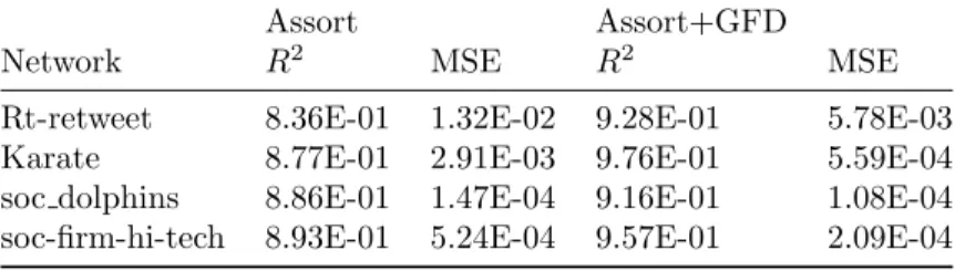
Table 3: Model comparison for predicting log number of events for SIS.
Assort Assort+GFD
Network R2
MSE R2
MSE
Rt-retweet 8.36E-01 1.32E-02 9.28E-01 5.78E-03
Karate 8.77E-01 2.91E-03 9.76E-01 5.59E-04
soc dolphins 8.86E-01 1.47E-04 9.16E-01 1.08E-04
Table 4: Model comparison for predicting log of largest eigenvalue.
Assort Assort+GFD
Network R2
MSE R2
MSE
Rt-retweet 8.51E-01 4.21E-05 9.50E-01 1.41E-05
Karate 8.66E-01 9.74E-06 9.78E-01 1.61E-06
soc dolphins 8.74E-01 3.98E-06 9.15E-01 2.69E-06
soc-firm-hi-tech 9.25E-01 2.82E-06 9.72E-01 1.04E-06
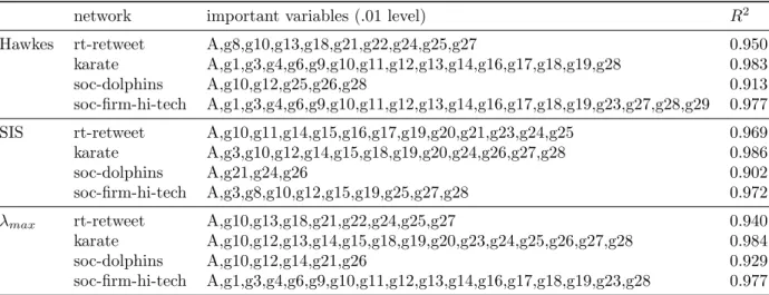
Table 5: Important variables along withR2
values for interaction regression model.
network important variables (.01 level) R2
Hawkes rt-retweet A,g8,g10,g13,g18,g21,g22,g24,g25,g27 0.950
karate A,g1,g3,g4,g6,g9,g10,g11,g12,g13,g14,g16,g17,g18,g19,g28 0.983
soc-dolphins A,g10,g12,g25,g26,g28 0.913
soc-firm-hi-tech A,g1,g3,g4,g6,g9,g10,g11,g12,g13,g14,g16,g17,g18,g19,g23,g27,g28,g29 0.977
SIS rt-retweet A,g10,g11,g14,g15,g16,g17,g19,g20,g21,g23,g24,g25 0.969
karate A,g3,g10,g12,g14,g15,g18,g19,g20,g24,g26,g27,g28 0.986
soc-dolphins A,g21,g24,g26 0.902
soc-firm-hi-tech A,g3,g8,g10,g12,g15,g19,g25,g27,g28 0.972
λmax rt-retweet A,g10,g13,g18,g21,g22,g24,g25,g27 0.940
karate A,g10,g12,g13,g14,g15,g18,g19,g20,g23,g24,g25,g26,g27,g28 0.984
soc-dolphins A,g10,g12,g14,g21,g26 0.929
soc-firm-hi-tech A,g1,g3,g4,g6,g9,g10,g11,g12,g13,g14,g16,g17,g18,g19,g23,g28 0.977
To improve the regression model in Eq. 9, we consider an interaction model where the statistically significant variables from Table 5 are used and interaction terms of the form A·
log(d(gi)) are added. In Table 5 we display theR2 values for this interaction model. In some cases we see large improvements, for example in the case of the retweet network and the Hawkes model the R2 value increases from .86 to .95 (the R2 for assortativity alone is .72). In the majority of cases theR2value of this interaction model is above .95 and for the karate model is above .98. TheR2value for the soc-dolphins network is slighly lower, .9 to .92. Given that only high order graphlets are selected in the soc-dolphins network, it may be the case that graphlets beyond g29 are needed to achieveR2 values close to 1 for that network.
5
Discussion
Our results show that Hawkes and SIS processes on networks with the same degree distribution and assortativity can exhibit very different levels of virality. With the inclusion of graphlets in predictive models of virality, R2 values improve by 10-20% depending on the network and specific process. These results have implications for prediction of real network viral processes, as current methods are generally based upon degree distribution alone [7, 32] and predictive accuracy may improve with graphlet based features. Here it may be beneficial to consider local graphlet statistics [8] around the source node of the process. For example, the local graphlet frequency around a Tweeter may help predict the number of re-shares of that user’s Tweet.
The statistically significant graphlets for a given network may also provide useful information for network optimization. When the goal is to reduce the spread of viruses, for example to mitigate fake news [11], one may wish to remove nodes in a way that leads to the greatest reduction in viral spreading. While degree may be used to make such selections, further gains
may be made by considering assortativity and graphlet frequency. For example, in the case of the dolphins-SIS simulation, choosing nodes that reduce the frequency of graphlets 21, 24, and 26 may provide a better mitigation strategy than other metrics like centrality or degree. These questions will be addressed in future research.
6
Acknowledgements
This work was supported in part by NSF grants SCC-1737585, SES-1343123, ATD-1737996, and ATD-1737925.
References
[1] Roy M Anderson, Robert M May, and B Anderson.Infectious diseases of humans: dynamics and control, volume 28. Wiley Online Library, 1992.
[2] Noam Berger, Christian Borgs, Jennifer T Chayes, and Amin Saberi. On the spread of viruses on the internet. InProceedings of the sixteenth annual ACM-SIAM symposium on Discrete algorithms, pages 301–310. Society for Industrial and Applied Mathematics, 2005. [3] Mansurul Bhuiyan, Mahmudur Rahman, Mahmuda Rahman, and Mohammad Al Hasan. GUISE: uniform sampling of graphlets for large graph analysis. In12th IEEE International Conference on Data Mining, ICDM 2012, Brussels, Belgium, December 10-13, 2012, pages 91–100, 2012.
[4] Duncan S Callaway, Mark EJ Newman, Steven H Strogatz, and Duncan J Watts. Net-work robustness and fragility: Percolation on random graphs. Physical review letters, 85(25):5468, 2000.
[5] Deepayan Chakrabarti, Yang Wang, Chenxi Wang, Jurij Leskovec, and Christos Falout-sos. Epidemic thresholds in real networks. ACM Trans. Inf. Syst. Secur., 10(4):1:1–1:26, January 2008.
[6] Deepayan Chakrabarti, Yang Wang, Chenxi Wang, Jurij Leskovec, and Christos Faloutsos. Epidemic thresholds in real networks. ACM Transactions on Information and System Security (TISSEC), 10(4):1, 2008.
[7] Riley Crane and Didier Sornette. Robust dynamic classes revealed by measuring the response function of a social system. Proceedings of the National Academy of Sciences, 105(41):15649–15653, 2008.
[8] Vachik Dave, Nesreen Ahmed, and Mohammad Al Hasan. E-CLoG: Counting edge-centric local graphlets. In Proceedings of the 2017 IEEE International Conference on Big Data (Big Data), BIG DATA ’17. IEEE Computer Society, 2017.
[9] Zolt´an Dezs˝o and Albert-L´aszl´o Barab´asi. Halting viruses in scale-free networks. Physical Review E, 65(5):055103, 2002.
[10] K Dietz. Models for vector-borne parasitic diseases. InVito Volterra Symposium on Math-ematical Models in Biology, pages 264–277. Springer, 1980.
[11] Mehrdad Farajtabar, Jiachen Yang, Xiaojing Ye, Huan Xu, Rakshit Trivedi, Elias Khalil, Shuang Li, Le Song, and Hongyuan Zha. Fake news mitigation via point process based intervention. InInternational Conference on Machine Learning, pages 1097–1106, 2017. [12] A. Ganesh, L. Massoulie, and D. Towsley. The effect of network topology on the spread of
epidemics. InProceedings IEEE 24th Annual Joint Conference of the IEEE Computer and Communications Societies., volume 2, pages 1455–1466 vol. 2, March 2005.
[13] Or Givan, Nehemia Schwartz, Assaf Cygelberg, and Lewi Stone. Predicting epidemic thresholds on complex networks: Limitations of mean-field approaches. Journal of the-oretical biology, 288:21–28, 2011.
[14] Christos Gkantsidis, Milena Mihail, and Ellen Zegura. The markov chain simulation method for generating connected power law random graphs. InIn Proc. 5th Workshop on Algorithm Engineering and Experiments (ALENEX). SIAM, 2003.
[15] Sarika Jalan and Alok Yadav. Assortative and disassortative mixing investigated using the spectra of graphs. Physical Review E, 91(1):012813, 2015.
[16] Yang L-X, Draief M, and Yang X. The impact of the network topology on the viral prevalence: A node-based approach. PLoS ONE, 10(7), 2015.
[17] Jure Leskovec, Lada A Adamic, and Bernardo A Huberman. The dynamics of viral mar-keting. ACM Transactions on the Web (TWEB), 1(1):5, 2007.
[18] Laszlo Lovasz. Eigenvalues of graphs. http://web.cs.elte.hu/~lovasz/eigenvals-x. pdf, 2007.
[19] Sergei Maslov and Kim Sneppen. Specificity and stability in topology of protein networks.
Science, 296(5569):910–913, 2002.
[20] M. E. J. Newman. The structure and function of complex networks. SIAM REVIEW, 45:167–256, 2003.
[21] Mark EJ Newman. Assortative mixing in networks. Physical review letters, 89(20):208701, 2002.
[22] Jing Qu, Sheng-Jun Wang, Marko Jusup, and Zhen Wang. Effects of random rewiring on the degree correlation of scale-free networks. Scientific reports, 5, 2015.
[23] Mahmudur Rahman and Mohammad Al Hasan. Link prediction in dynamic networks using graphlet. InJoint European Conference on Machine Learning and Knowledge Discovery in Databases, pages 394–409. Springer, 2016.
[24] Mahmudur Rahman, Mansurul Bhuiyan, and Mohammad Al Hasan. GRAFT: an approx-imate graphlet counting algorithm for large graph analysis. In 21st ACM International Conference on Information and Knowledge Management, CIKM’12, Maui, HI, USA, Oc-tober 29 - November 02, 2012, pages 1467–1471, 2012.
[25] Mahmudur Rahman, Mansurul Alam Bhuiyan, and Mohammad Al Hasan. GRAFT: An efficient graphlet counting method for large graph analysis. IEEE Trans. Knowl. Data Eng., 26(10):2466–2478, 2014.
[26] Mahmudur Rahman, Mansurul Alam Bhuiyan, Mahmuda Rahman, and Mohammad Al Hasan. GUISE: a uniform sampler for constructing frequency histogram of graphlets.
Knowledge and Information Systems, 38(3):511–536, 2014. Invited: best papers of ICDM’12.
[27] Mahmudur Rahman and Mohammad Al Hasan. Sampling triples from restricted net-works using MCMC strategy. InProceedings of the 23rd ACM International Conference on Conference on Information and Knowledge Management, CIKM 2014, Shanghai, China, November 3-7, 2014, pages 1519–1528, 2014.
[28] Ryan A. Rossi and Nesreen K. Ahmed. The network data repository with interactive graph analytics and visualization. In Proceedings of the Twenty-Ninth AAAI Conference on Artificial Intelligence, 2015.
[29] Tanay Kumar Saha and Mohammad Al Hasan. Finding network motifs using MCMC sampling. InComplex Networks VI - Proceedings of the 6th Workshop on Complex Networks CompleNet 2015, New York City, USA, March 25-27, 2015, pages 13–24, 2015.
[30] M. B. Short, G. O. Mohler, P. J. Brantingham, and G. E. Tita. Gang rivalry dynamics via coupled point process networks. Discrete and Continuous Dynamical Systems - Series B, 19(5):1459–1477, 2014.
[31] Piet Van Mieghem, Huijuan Wang, Xin Ge, Siyu Tang, and FA Kuipers. Influence of assortativity and degree-preserving rewiring on the spectra of networks. The European Physical Journal B-Condensed Matter and Complex Systems, 76(4):643–652, 2010.
[32] Qingyuan Zhao, Murat A Erdogdu, Hera Y He, Anand Rajaraman, and Jure Leskovec. Seismic: A self-exciting point process model for predicting tweet popularity. InProceedings of the 21th ACM SIGKDD International Conference on Knowledge Discovery and Data Mining, pages 1513–1522. ACM, 2015.