An Evolutionary Algorithm for Large-Scale Sparse Multi-Objective Optimization Problems

(1)

An Evolutionary Algorithm for Large-Scale

Sparse Multi-Objective Optimization Problems

Ye Tian, Xingyi Zhang,

Senior Member, IEEE

, Chao Wang, and Yaochu Jin,

Fellow, IEEE

Abstract—In the last two decades, a variety of different types of multi-objective optimization problems (MOPs) have been extensively investigated in the evolutionary computa-tion community. However, most existing evolucomputa-tionary algo-rithms encounter difficulties in dealing with MOPs whose Pareto optimal solutions are sparse (i.e., most decision vari-ables of the optimal solutions are zero), especially when the number of decision variables is large. Such large-scale sparse MOPs exist in a wide range of applications, for example, feature selection that aims to find a small subset of features from a large number of candidate features, or structure op-timization of neural networks whose connections are sparse to alleviate overfitting. This paper proposes an evolutionary algorithm for solving large-scale sparse MOPs. The proposed algorithm suggests a new population initialization strategy and genetic operators by taking the sparse nature of the Pareto optimal solutions into consideration, to ensure the sparsity of the generated solutions. Moreover, this paper also designs a test suite to assess the performance of the proposed algorithm for large-scale sparse MOPs. Experimental results on the proposed test suite and four application examples demonstrate the superiority of the proposed algorithm over seven existing algorithms in solving large-scale sparse MOPs. Index Terms—Large-scale multi-objective optimization, evolutionary algorithm, sparse Pareto optimal solutions, fea-ture selection, evolutionary neural network

I. INTRODUCTION

M

ULTI-objective optimization problems (MOPs) re-fer to those having multiple objectives to be op-timized simultaneously [1]. For example, the portfolio

Manuscript received –. This work was supported in part by the National Natural Science Foundation of China under Grant 61672033, 61822301, 61876123, and U1804262, in part by the State Key Laboratory of Synthetical Automation for Process Industries under Grant PAL-N201805, and in part by the Anhui Provincial Natural Science Founda-tion under Grant 1808085J06 and 1908085QF271.(Corresponding author: Xingyi Zhang)

Y. Tian is with the Key Laboratory of Intelligent Computing and Signal Processing of Ministry of Education, Institutes of Physical Science and Information Technology, Anhui University, Hefei 230601, China. (email: field910921@gmail.com)

X. Zhang and C. Wang are with the Key Laboratory of Intelligent Computing and Signal Processing of Ministry of Education, School of Computer Science and Technology, Anhui University, Hefei 230601, China. (email: xyzhanghust@gmail.com; wangchao8@ahu.edu.cn)

Y. Jin is with the Department of Computer Science, University of Surrey, Guildford, Surrey, GU2 7XH, U.K.. He is also with the Department of Computer Science and Engineering, Southern Uni-versity of Science and Technology, Shenzhen 518055, China. (email: yaochu.jin@surrey.ac.uk)

optimization problem is to maximize return and mini-mize risk [2], the next release problem is to maximini-mize customer satisfaction and minimize cost [3], and the community detection problem is to maximize intra-link density and minimize inter-link density [4]. Since the objectives of an MOP are usually conflicting with each other, there does not exist a single solution simultane-ously optimizing all objectives; instead, a number of solutions can be obtained as trade-offs between different objectives, known as Pareto optimal solutions. All the Pareto optimal solutions for an MOP constitute the Pareto set, and the image of the Pareto set in objective space is called the Pareto front.

Since the first implementation of a multi-objective evolutionary algorithm (MOEA) [5], a variety of different types of MOPs have been considered for evolutionary algorithms [6]. In many real-world applications, there exists a type of MOPs whose Pareto optimal solutions are sparse, i.e., most decision variables of the optimal solutions are zero. For example, the feature selection problem in classification [7] aims to choose a small num-ber of relevant features to achieve the best classification performance, by means of minimizing both the number of selected features and classification error. In general, the features in Pareto optimal solutions account for a small portion of all candidate features [8]. Therefore, if binary encoding is adopted (i.e., each binary decision variable indicates whether one feature is selected or not), most decision variables of the Pareto optimal solutions will be zero, in other words, the Pareto optimal solutions are sparse. Such subset selection problems with sparse Pareto optimal solutions are commonly seen in many other applications, for instance, sparse regression [9], pattern mining [10], and critical node detection [11].

The Pareto optimal solutions of some MOPs with real variables are also sparse, such as neural network training [12], sparse reconstruction [13], and portfolio optimization [2]. For instance, in order to alleviate over-fitting as well as improve the interpretability of the learned network, training neural network should not only consider the approximation performance, but also control the complexity of the model [14]. For this aim, many approaches such as lasso [15], sparse coding [16], and dropout [17] have been proposed, which can be regarded as a feature selection and model construction process done simultaneously. From the perspective of 0000–0000/00$00.00 c⃝0000 IEEE

(2)

0 0.05 0.1 0.15 0.2 0.25 0.3

Ratio of selected features

0 0.2 0.4 0.6 0.8 1

Error rate on validation set

NSGA-II SPEA2 SMS-EMOA EAG-MOEA/D SFS

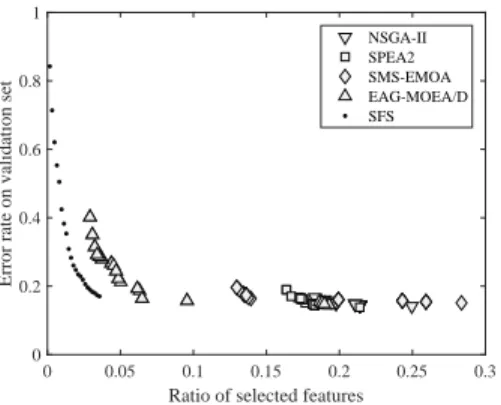
Fig. 1. Solution sets obtained by NSGA-II, SPEA2, SMS-EMOA, EAG-MOEA/D, and SFS (a greedy approach) on a feature selection problem with 617 decision variables. Although the four MOEAs consume more runtime than SFS, SFS significantly outperforms the four MOEAs in terms of both error rate and ratio of selected features.

multi-objective optimization, training neural network is usually regarded as a bi-objective MOP, i.e., minimizing both training error and model complexity [18]. Therefore, the Pareto optimal solutions will be sparse if the weights of the neural network are directly encoded in solutions. Although sparse MOPs widely exist in many popular applications, such type of MOPs has not been exclusively investigated before. In fact, few MOEAs are dedicated to solving sparse MOPs, while most work only adopts general MOEAs to solve them [19], [20]. As reported in the literature, many existing MOEAs encounter dif-ficulties in dealing with sparse MOPs, especially when the number of decision variables is large [21], [22]. For example, Fig. 1 plots the solution sets obtained by four MOEAs (i.e., NSGA-II [23], SPEA2 [24], SMS-EMOA [25], and EAG-MOEA/D [26]) and a greedy approach (i.e., sequential forward selection, SFS [27]) on a fea-ture selection problem with 617 decision variables. It is obvious that the solutions obtained by the MOEAs are worse than those obtained by the greedy approach, even though the MOEAs consume more runtime than the greedy approach. Some algorithms with customized search strategies have been proposed for solving specific sparse MOPs [21], [28], but they cannot be employed to solve other sparse MOPs directly. On the other hand, although some MOEAs have been tailored for large-scale MOPs [29]–[31], they cannot be applied to large-scale sparse MOPs with binary variables since these MOEAs are based on decision variable division and only effective in solving MOPs with real variables.

Existing MOEAs are ineffective for large-scale sparse MOPs mainly because they do not consider the sparse nature of Pareto optimal solutions when evolving the population. For example, most existing MOEAs ran-domly initialize the population and make each decision variable be 0 or 1 with the same probability. However, since most decision variables of the Pareto optimal so-lutions for sparse MOPs are 0, the initial population generated by existing MOEAs is far away from the Pareto set, and many computational resources should

be consumed for approximating the Pareto set in a large decision space. For the bitwise mutation used in existing MOEAs, each decision variable has the same probability to be flipped, so the decision variables of offsprings are expected to have the same number of 0 and 1. Therefore, the bitwise mutation is likely to pull the offsprings away from the Pareto set of sparse MOPs.

Since many sparse MOPs are pursued based on a large dataset, the objective functions of them contain a large number of decision variables and are computation-ally expensive, which poses stiff challenges to existing MOEAs to obtain satisfactory solutions within a tight budget on computational cost. To address this issue, this paper proposes an MOEA for solving large-scale sparse MOPs. The main contributions of this paper are summarized as follows.

1) We propose an MOEA for solving large-scale sparse MOPs. The proposed algorithm ensures the sparsity of solutions by a new population initial-ization strategy and genetic operators, which are verified to be effective in approximating sparse Pareto optimal solutions.

2) We design a multi-objective test suite for assessing the performance of the proposed algorithm, which contains eight benchmark problems with adjustable sparsity of Pareto optimal solutions.

3) We perform experiments on the proposed test suite and four application examples. The statistical re-sults verify that the proposed algorithm exhibits significantly better performance than seven exist-ing MOEAs in solvexist-ing large-scale sparse MOPs. The rest of this paper is organized as follows. Section II introduces sparse MOPs in applications and existing MOEAs for sparse MOPs. Section III details the proposed algorithm for large-scale sparse MOPs, and Section IV presents the proposed sparse multi-objective test suite. The experimental results on the proposed test suite and the applications are given in Sections V and VI. Finally, conclusions are drawn in Section VII.

II. SPARSEMULTI-OBJECTIVEOPTIMIZATION PROBLEMS

A. Sparse MOPs in Large-Scale Optimization Problems

There exist many real-world optimization problems containing a large number of decision variables, which are known as large-scale optimization problems (LOPs). Due to the exponentially increased search space of LOPs, they cannot be easily solved by general evolutionary algorithms, hence some novel techniques have been adopted to tackle specific types of LOPs, such as variable interaction analysis [32]–[34], linkage learning [35], and random embedding based Bayesian optimization [36], [37]. For the LOPs in many important fields including machine learning [18], data mining [10], and network science [11], many problems contain sparse optimal solu-tions. However, no technique has been tailored for sparse problems before.

(3)

'XKRK\GTZLKGZ[XKY[HYKZ Hair, Eggs, Milk

(KGX

Hair: True Feathers: False Eggs: False Airborne: False Toothed: True Backbone: True Fins: False Venomous: False Legs: Four Milk: True

,XUM

Hair: False Feathers: False Eggs: True Airborne: False Toothed: True Backbone: True Fins: False Venomous: False Legs: Four Milk: False )UXXKYVUTJOTMYUR[ZOUT 1 0 0 0 0 0 1 0 1 0

(a) The feature selection problem. The features

Hair,Eggs, andMilkare relevant features since they can be used to distinguish the two animals.

1. Hat, Scarf, Gloves, Handbag, Belt, Heels 2. Hat, Scarf, Gloves, Necklace

3. Necklace 4. Hat, Scarf, Gloves

5. Hat, Scarf, Handbag, Belt, Heels 6. Hat, Scarf, Gloves

'XKRK\GTZLKGZ[XKY[HYKZ )UXXKYVUTJOTMYUR[ZOUT

Hat, Scarf, Gloves

1 1 1 0 0 0 0

(b) The pattern mining problem. The items Hat,

Scarf, andGlovesconstitute a recommended pattern since this pattern occurs in four shopping lists.

Critical nodes

)UXXKYVUTJOTMYUR[ZOUT 0 0 0 0 0 0 1 1 0 0 0 0 0

(c) The critical node detection problem. The two filled circles are critical nodes since the graph will be split into four disconnected components if they are deleted. Weights /TV[ZRG_KX .OJJKTRG_KX 5[ZV[ZRG_KX Weights )UXXKYVUTJOTMYUR[ZOUT 0.3 0 0 0 0.1 0.1 0.4 0 0.2 0 0 0.1

(d) The neural network training problem. It aims to optimize the weights of a neural network for minimizing the complexity and error.

Fig. 2. Examples of four sparse MOPs in applications.

It is noteworthy that LOPs with a low intrinsic dimen-sionality [38] are similar to sparse LOPs to some extent, but the optimal solutions of these two types of problems are significantly different. For sparse LOPs, only a small portion of decision variables contribute to the optimal solutions, and the noncontributing decision variables should be set to 0. By contrast, only a small portion of decision variables contribute to the objective functions of LOPs with a low intrinsic dimensionality, while the noncontributing decision variables can be arbitrary val-ues. Therefore, sparse LOPs are more difficult than LOPs with a low intrinsic dimensionality since all the decision variables in sparse LOPs should be optimized.

In this paper, we concentrate on the sparse problems in large-scale MOPs. Although there exist some sparse single-objective optimization problems (SOPs), we do not consider them due to the following two reasons. First, many sparse SOPs embed the sparsity of solutions in the objective function [15], [39], which can actually be regarded as the second objective to be optimized; that is, sparse SOPs can be converted into sparse MOPs. Second, the optimal solutions of some problems are sparse only if multiple conflicting objectives are considered [2], [10].

B. Four Sparse MOPs in Applications

Four popular sparse MOPs in applications are intro-duced in the following, namely, feature selection [8], pattern mining [10], critical node detection [11], and neural network training [18]. These four problems are described in Fig. 2, and the mathematical definition of them can be found in Supplementary Materials I.

The feature selection problem. For classification tasks, a large number of features are usually introduced to the dataset, where many features are irrelevant or redun-dant. The aim of feature selection is to choose only relevant features for classification, which can not only reduce the number of features, but also improve the clas-sification performance [7]. Therefore, feature selection is inherently a bi-objective MOP, and some MOEAs have been employed to solve it [8], [19].

The pattern mining problem.This problem seeks to find the most frequent and complete pattern (i.e., a set of items) from a transaction dataset, where a transaction dataset contains a set of transactions and each trans-action contains a set of items. For example, when a customer is purchasing one item on a Website, the task

(4)

is to recommend the matching items to the customer, by means of mining the best pattern from all the historical shopping lists. In [21], the pattern mining problem is regarded as an MOP for maximizing both the frequency and completeness, where the frequency of a pattern indicates the ratio of transactions it occurs in, and the completeness of a pattern indicates its occupancy rate in the transactions it occurs in.

The critical node detection problem. Given a graphG= (V, E), the critical node detection problem [11] is to select a point set x ⊆ V, the deletion of which minimizes pairwise connectivity in the remaining graph G[V\x]. In order to select fewer points for larger destruction to the graph, both the number of selected points and the pairwise connectivity in the remaining graph should be minimized. As a result, the critical node detection problem is also a subset selection MOP, and has been tackled by some MOEAs [40], [41].

The neural network training problem. Evolutionary al-gorithms have been deeply studied for training artifi-cial neural network, such as optimizing topology [42], weights [43], and hyperparameters [20] of the network. Regarding multi-objective approaches, various objectives have been considered in training neural network [18], [44], [45]. In order to control the complexity of neural network, in this paper we adopt the definition suggested in [18], i.e., optimizing the weights of a feedforward neural network for minimizing the complexity and error. Although the above four MOPs are from different fields and contain different objectives, they can be grouped into the same category of MOPs since the Pareto optimal solutions of them are sparse. For the problems of feature selection, critical node detection, and neural network training, the sparsity of solution is defined as an objective to be optimized directly, hence the Pareto optimal solutions are certainly sparse. While for the pattern mining problem which does not explicitly control the sparsity of solution, the Pareto optimal solutions are also sparse due to the definition of the objectives. In general, the number of items in each transaction is much fewer than the total number of items in the dataset, hence the items in each Pareto optimal solution should account for a small portion of all the items, otherwise the solution will not occur in any transaction.

C. MOEAs for Sparse MOPs and Large-Scale MOPs

For the above sparse MOPs, most work solves them via existing MOEAs like NSGA-II [23], SMS-EMOA [25], and MOEA/D [46], and some work also enhances the performance by adopting customized search strategies. For example, Gu et al. [47] modified the competitive swarm optimizer and embedded it in a wrapper ap-proach for feature selection, Zhang et al.[21] suggested a novel population initialization strategy in NSGA-II to solve the pattern mining problem, Aringhieri et al.

[28] made use of appropriate greedy rules in genetic operators to improve the quality of offsprings for critical

node detection, and Sun et al. [48] assumed a set of orthogonal vectors to highly reduce the number of deci-sion variables in training an unsupervised deep neural network. However, it is worth noting that these cus-tomized search strategies cannot be employed to solve other sparse MOPs directly, since they are related to the objective functions and the structure of dataset, which can only solve a specific type of sparse MOPs.

On the other hand, many MOEAs tailored for large-scale MOPs cannot be applied to the feature selection problem, the pattern mining problem, and the critical node detection problem with binary variables, since most of these MOEAs are based on decision variable division. For example, MOEA/DVA [29] and LMEA [30] divided the decision variables by control property analysis and variable clustering, respectively, both of which perturbed every decision variable in the continuous decision space. WOF [31] divided the decision variables into several groups, and optimized a weight vector instead of all the decision variables in the same group. As a result, these MOEAs can only solve MOPs with real variables. Be-sides, a large number of function evaluations should be consumed for dividing the decision variables, which is inefficient for solving sparse MOPs with a large dataset. To address the above issues, this paper proposes an MOEA for large-scale sparse MOPs. The proposed al-gorithm does not need to know the objective functions or the dataset, and it can solve both MOPs with real variables and MOPs with binary variables.

III. ANEVOLUTIONARYALGORITHM FORSPARSE MULTI-OBJECTIVEOPTIMIZATIONPROBLEMS

A. Framework of the Proposed SparseEA

As shown in Algorithm 1, the proposed evolutionary algorithm for large-scale sparse MOPs, called SparseEA, has a similar framework to NSGA-II [23]. First of all, a population P with size N is initialized, and the non-dominated front number [49] and crowding distance [23] of each solution in P are calculated. In the main loop, 2N parents are selected by binary tournament selection according to the non-dominated front number and crowding distance of each solution in P. Then N offsprings are generated (i.e., two parents are used to generate one offspring) and combined with P. After-wards, the duplicated solutions in the combined pop-ulation are deleted, and N solutions with better non-dominated front number and crowding distance in the combined population survive to the next generation.

In short, the mating selection and environmental selec-tion in SparseEA are similar to those in NSGA-II, while SparseEA uses new strategies to generate the initial population and offsprings, which can ensure the sparsity of the generated solutions. The population initialization strategy and genetic operators in SparseEA are elabo-rated in the next two subsections respectively.

(5)

Algorithm 1:Framework of the proposed SparseEA Input:N (population size)

Output:P (final population)

1 [P, Score]←Initialization(N); //Algorithm 2

2 [F1, F2, . . .]←Do non-dominated sorting onP;

3 CrowdDis←CrowdingDistance(F);

4 whiletermination criterion not fulfilleddo

5 P′←Select2N parents via binary tournament

selection according to the non-dominated front

number and CrowdDisof solutions inP;

6 P ←P∪V ariation(P′, Score);//Algorithm 3

7 Delete duplicated solutions fromP;

8 [F1, F2, . . .]←Do non-dominated sorting onP;//Fi

denotes the solution set in the i-th

non-dominated front 9 CrowdDis←CrowdingDistance(F); 10 k←argmini|F1 ∪ . . .∪Fi| ≥N; 11 Delete|F1 ∪

. . .∪Fk| −N solutions fromFk with the

smallestCrowdDis;

12 P ←F1 ∪

. . .∪Fk; 13 returnP;

B. Population Initialization Strategy of SparseEA

The proposed SparseEA are designed for solving sparse MOPs with real variables and binary variables. To this end, a hybrid representation of solution is adopted to integrate the two different encodings, which has been widely used for solving many problems such as neural network training [43] and portfolio optimization [50]. Specifically, a solution x in SparseEA consists of two components, i.e., a real vectordecdenoting the decision variables and a binary vector mask denoting the mask. The final decision variables ofxfor calculating objective values are obtained by

(x1, x2, . . .) = (dec1×mask1, dec2×mask2, . . .). (1)

For instance, for a real vectordec= (0.5,0.3,0.2,0.8,0.1) and a binary vector mask = (1,0,0,1,0), the decision variables are (0.5,0,0,0.8,0). During the evolution, the real vector dec of each solution can record the best decision variables found so far, while the binary vector mask can record the decision variables that should be set to zero, thereby controlling the sparsity of solutions. Note that the real vector dec is always set to a vector of ones if the decision variables are binary numbers, so that the final decision variables can be either 0 or 1 depending on the binary vector mask. In SparseEA, the dec and mask of each solution are generated and evolved by different strategies.

The population initialization strategy of SparseEA is presented in Algorithm 2, which consists of two steps, i.e., calculating the scores of decision variables and generating the initial population. To begin with, a population Q with D solutions is generated, where D denotes the number of decision variables. Specifically, the elements in the real vector dec of each solution are set to random values, while the elements in the binary vector maskare set to 0, except that thei-th element in the mask of the i-th solution is set to 1. Therefore, the

Algorithm 2: Initialization(N) Input:N (population size)

Output:P (initial population),Score(scores of decision variables)

//Calculate the scores of variables

1 D←Number of decision variables;

2 ifthe decision variables are real numbersthen

3 Dec←D×D random matrix;

4 else ifthe decision variables are binary numbersthen

5 Dec←D×D matrix of ones;

6 M ask←D×D identity matrix;

7 Q←A population whosei-th solution is generated by

thei-th rows ofDecandM askaccording to (1);

8 [F1, F2, . . .]←Do non-dominated sorting on Q;

9 fori= 1toD do

10 Scorei←k, s.t.Qi∈Fk;//Qi denotes the i-th

solution in Q

//Generate the initial population

12 Dec←Uniformly randomly generate the decision

variables ofN solutions;

13 else ifthe decision variables are binary numbersthen

14 Dec←N×Dmatrix of ones;

15 M ask←N×Dmatrix of zeros;

16 fori= 1toN do

17 forj= 1torand()×D do

18 [m, n]←Randomly select two decision varaibles;

19 ifScorem< Scoren then

20 Set them-th element in thei-th binary vector

inM askto 1;

21 else

22 Set then-th element in thei-th binary vector

inM askto 1;

23 P←A population whosei-th solution is generated by

thei-th rows ofDecandM askaccording to (1);

24 returnP andScore;

binary vectorsmaskof all the solutions inQconstitute a D×D identity matrix. Then, the populationQis sorted by non-dominated sorting, and the non-dominated front number of the i-th solution is regarded as the score of the i-th decision variable. As a consequence, the score of a decision variable indicates the probability that it should be set to zero, where a smaller score can indicate a lower probability that the decision variable should be set to zero, since a lower non-dominated front number indicates a better quality of solution. The scores of de-cision variables will be involved in both the population initialization strategy and genetic operators in SparseEA, where the elements in mask to be flipped are selected by binary tournament selection according to the scores of decision variables.

It is worth noting that more precise score assignment strategy can be adopted for the decision variables, e.g., by considering the interaction between variables [35] and updating the scores during the evolution. Nevertheless, the proposed score assignment strategy is empirically verified to be effective in solving sparse MOPs, and we use this score assignment strategy in SparseEA based

(6)

0.1 0.2 0.3 0.4 0.5

0.2 0.25 0.3 0.35 0.4 0.45

The proposed initialization strategy Random initialization strategy

Fig. 3. Two populations generated by the proposed initialization strategy and by random initialization strategy, where each population contains 50 solutions for a feature selection problem (i.e., FS4 in

Table II) _.

on the following two considerations. First, the proposed score assignment strategy works very efficiently, which consumes only D function evaluations. Second, the bi-nary vector mask is generated by binary tournament selection according to the scores of decision variables, where the randomness in binary tournament selection is helpful for the effectiveness of the score assignment strategy.

On the other hand, some existing algorithms also use a real value to represent the probability of a variable being 0 or 1 [51], [52], but the score in SparseEA is completely different. To be specific, the probability of each variable being 0 or 1 is directly encoded in the solutions of existing algorithms, which will be optimized during the evolutionary process. By contrast, the score of each variable in SparseEA is estimated beforehand, which is used to guide the optimization of solutions.

After calculating the scores of decision variables, the initial population P is generated. For each solution in P, each element in the real vectordecis set to a random value, and each element in the binary vectormaskis set to 0. Then,rand()×Delements are selected from mask via binary tournament selection according to the scores of decision variables (the smaller the better) and set to 1, whererand()denotes a uniformly distributed random number in [0,1]. Fig. 3 plots a population generated by SparseEA and a randomly generated population in objective space, where each population contains 50 solu-tions for a feature selection problem. It can be observed that the population generated by SparseEA has better convergence and diversity than the randomly generated population, hence the effectiveness of the proposed pop-ulation initialization strategy is verified.

C. Genetic Operators of SparseEA

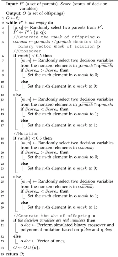
Algorithm 3 details the genetic operators in SparseEA, where two parents pand qare randomly selected from P′ to generate an offspring o each time. The binary vector mask of o is first set to the same to that of p, then either the following two operations is performed

Algorithm 3: V ariation(P′, Score)

Input:P′ (a set of parents),Score(scores of decision variables)

Output:O(a set of offsprings)

1 O← ∅;

2 whileP′ is not emptydo

3 [p,q]←Randomly select two parents fromP′;

4 P′←P′\ {p,q};

//Generate the mask of offspring o

5 o.mask←p.mask;//p.mask denotes the

binary vector mask of solution p

//Crossover

6 ifrand()<0.5then

7 [m, n]←Randomly select two decision variables

from the nonzero elements inp.mask∩q.mask;

8 ifScorem> Scoren then

9 Set them-th element ino.maskto 0;

10 else

11 Set then-th element ino.maskto 0;

12 else

from the nonzero elements inp.mask∩q.mask;

16 else

//Mutation

18 ifrand()<0.5then

from the nonzero elements ino.mask;

20 ifScorem> Scoren then

22 else

24 else

from the nonzero elements ino.mask;

28 else

//Generate the dec of offspring o

31 o.dec←Perform simulated binary crossover and

polynomial mutation based onp.decandq.dec;

32 else

33 o.dec←Vector of ones;

34 O←O∪ {o}; 35 returnO;

with the same probability: selecting an element from the nonzero elements in p.mask ∩q.mask via binary tournament selection according to the scores of decision variables (the larger the better), and setting this element in the mask of o to 0; or selecting an element from the nonzero elements in p.mask ∩q.mask via binary tournament selection according to the scores of decision variables (the smaller the better), and setting this element in the mask of o to 1. Afterwards, the mask of o is

(7)

0.1 0.11 0.12 0.13 0.14 0.15

0.21 0.22 0.23 0.24 0.25 0.26 0.27

The proposed crossover and mutation Single-point crossover and bitwise mutation Parents

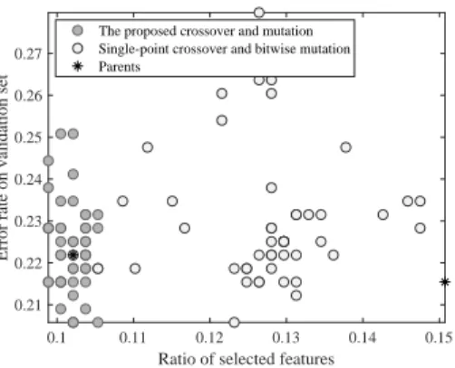
Fig. 4. Two sets of offsprings generated by the proposed crossover and mutation and by single-point crossover and bitwise mutation, where each set contains 50 offsprings for a feature selection problem (i.e., FS4

in Table II) _.

mutated by either the following two operations with the same probability: selecting an element from the nonzero elements in o.mask via binary tournament selection according to the scores of decision variables (the larger the better), and setting this element to 0; or selecting an element from the nonzero elements ino.maskvia binary tournament selection according to the scores of decision variables (the smaller the better), and setting this element to 1. The real vector dec of ois generated by the same operators to many existing MOEAs, i.e., simulated bi-nary crossover [53] and polynomial mutation [54]. Note that the dec ofois always set to a vector of ones if the decision variables are binary numbers.

To summarize, the proposed SparseEA adopts existing genetic operators for real variables, while it uses new genetic operators for binary variables. In fact, some specific operators have been designed for binary vari-ables [55], [56]. It should be noted, however, that the genetic operators in SparseEA are tailored for sparse MOPs. Specifically, the proposed genetic operators flip one element in the zero elements or the nonzero elements in the binary vector mask with the same probability, where the element to be flipped is selected based on the scores of decision variables. Therefore, the offsprings generated by the proposed SparseEA are not expected to have the same number of 0 and 1, and the sparsity of the offsprings can be ensured. Fig. 4 plots a set of offsprings generated by SparseEA and a set of offsprings generated by most existing MOEAs (i.e., using single-point crossover and bitwise mutation) in objective space, where each set contains 50 offsprings generated by the same parents for a feature selection problem. Note that there exist some duplicated offsprings in the figure. As shown in Fig. 4, most offsprings generated by existing MOEAs locate between the two parents, while some offsprings generated by SparseEA can dominate both the two parents. Therefore, the effectiveness of the proposed genetic operators can be confirmed.

In order to empirically assess the performance of the proposed SparseEA for large-scale sparse MOPs, a test

suite containing eight sparse MOPs is designed in the next section.

IV. A SPARSEMULTI-OBJECTIVETESTSUITE

A. Sparse MOPs in Existing Test Suites

There exist many multi-objective benchmark prob-lems in the literature [57], but most of them do not concern the sparsity of Pareto optimal solutions. For example, the DTLZ test suite [58] contains seven un-constrained MOPs, where the Pareto set of DTLZ1– DTLZ5 is[0,1]M−1_{× {}₀_.₅_}D−M+1 _{and the Pareto set of}

DTLZ6 and DTLZ7 is [0,1]M−1_{× {}₀_}D−M+1_{, with} _M

denoting the number of objectives and D denoting the number of decision variables. Hence, only the Pareto optimal solutions of DTLZ6 and DTLZ7 are sparse. For the ZDT test suite [59], ZDT1–ZDT4 and ZDT6 have a sparse Pareto set of [0,1]× {0}D−1. For the WFG test suite [60], WFG1–WFG9 have various transformation functions between decision space and objective space, but all the Pareto optimal solutions are not sparse. As for other test suites with complicated Pareto sets [61], [62], few MOPs in them have sparse Pareto optimal solutions. In spite of some sparse MOPs in existing multi-objective test suites, most of them do not have a suitable hardness to study the performance of MOEAs for sparse MOPs. Specifically, for some MOPs like ZDT1–ZDT4 and ZDT6, they are relatively easy to be solved since the lower boundary of the decision variables is 0, which can be easily found by some operators [63]. As for some other MOPs like DTLZ6 and DTLZ7, they are quite difficult to be solved due to their complex Pareto fronts [64]. More importantly, the above MOPs do not have an adjustable sparsity of Pareto optimal solutions, and there does not exist linkage between decision variables. There-fore, for better assessing the performance of the pro-posed SparseEA, eight challenging but solvable MOPs with adjustable sparsity of Pareto optimal solutions are proposed in the following.

B. Formulation of the Proposed Test Suite

The MOPs in the proposed test suite have the follow-ing formulation: Minimize f1(x) =h1(x)(1 +gns(x) +gs(x)) f2(x) =h2(x)(1 +gns(x) +gs(x)) . . . fM(x) =hM(x)(1 +gns(x) +gs(x)) s.t. x= (x1, x2, . . . , xD) x1, x2, . . . , xM−1∈[0,1] xM, xM+1, . . . , xM+K−1∈[−1,2] xM+K, xM+K+1, . . . , xD∈[−1,2] , (2)

where f1, f2, . . . , fM are the objective functions and x

is the decision vector. The decision vector consists of three parts, wherex1, . . . , xM−1 are related to functions

(8)

h1, h2, . . . , hM, xM, . . . , xM+K−1 are related to function

gns, and xM+K, . . . , xD are related to function gs. Note that all of the proposed MOPs are with real variables, so the MOEAs using specific operators (e.g., particle swarm optimization [65], differential evolution [66], and estimation of distribution algorithm [67]) can be tested on them.

Functions h1, h2, . . . , hM ∈ [0,1] are known as the

shape functions, which determine the shape of Pareto front. Functions gns, gs≥0 are known as the landscape functions, which determine the fitness landscape. A so-lution for the proposed MOPs can be Pareto optimal only if gns = 0 and gs = 0, where gns can be 0 when xM, . . . , xM+K−1are set to particular values, and gscan be 0 whenxM+K, . . . , xDare set to 0. Therefore, the spar-sity of Pareto optimal solutions lies in the fact that the decision variables xM+K, . . . , xD of the Pareto optimal

solutions are always 0. In addition, the parameter K is determined by

K=⌈θ(D−M+ 1)⌉, (3) where θ∈[0,1]is a parameter determining the sparsity of Pareto optimal solutions. A smaller value of θ indi-cates a higher sparsity of Pareto optimal solutions.

C. An Example Problem

In order to create sparse MOPs based on the formu-lation given in (2), the shape functions and landscape functions should be defined. For example, the shape functions can be_         h1(x) =x1x2. . . xM₋1 h2(x) =x1x2. . .(1−xM−1) . . . hM(x) = 1−x1 , (4)

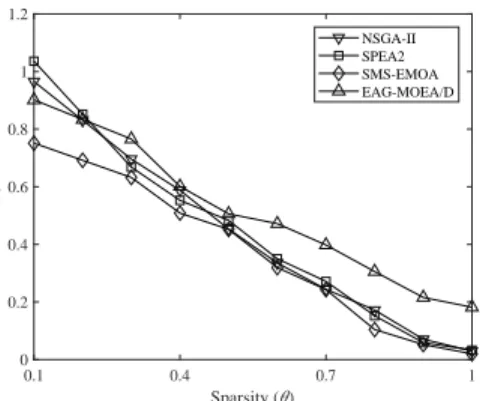
which defines a linear Pareto front. And the landscape functions can be gns(x) = ∑M+K−1 i=M (xi−π/3)2 gs(x) =∑_iD₌−_M1₊_K(xi−0.9xi+1)2+ (xD−0.9xM+K)2 . (5) Obviously, gns can be 0 only when xi = π/3 for M ≤ i ≤ M +K −1, and gs can be 0 only when xi= 0.9xi+1forM+K≤i≤D−1andxD= 0.9xM+K, i.e., xi should be set to 0 for all M +K ≤ i ≤ D. As a result, the Pareto set of this example MOP is [0,1]M−1_{× {}_π/₃_}K_{× {}₀_}D−M+1−K_{, and the Pareto} opti-mal solutions are sparse whenK is set to a small value. Fig. 5 plots the IGD values obtained by NSGA-II, SPEA2, SMS-EMOA, and EAG-MOEA/D on the exam-ple MOP averaged over 30 runs, where the number of objectivesM is set to 2, the number of decision variables is set to 100, and the sparsity of Pareto optimal solutions θ is ranged from 0.1 to 1. It can be seen from the figure that the four MOEAs exhibit worse performance if the MOP has sparser Pareto optimal solutions (i.e., a smaller value ofθ), hence it is confirmed that the example MOP

0.1 0.4 0.7 1 Sparsity ( ) 0 0.2 0.4 0.6 0.8 1 1.2 IGD NSGA-II SPEA2 SMS-EMOA EAG-MOEA/D

Fig. 5. Average IGD values obtained by NSGA-II, SPEA2, SMS-EMOA, and EAG-MOEA/D on the example MOP, where the sparsity of Pareto optimal solutions is ranged from 0.1 to 1 with an increment of 0.1. poses challenges to existing MOEAs in obtaining sparse solutions.

D. Eight Benchmark Problems SMOP1–SMOP8

Now we implement eight benchmark problem SMOP1–SMOP8 by defining different shape functions and landscape functions. On one hand, since the pro-posed test suite focuses on testing the performance of algorithms in finding sparse Pareto optimal solutions, three simple Pareto fronts (i.e., sets of shape functions) taken from DTLZ [58] and WFG [60] are adopted in SMOP1–SMOP8, namely, the linear Pareto front, the convex Pareto front, and the concave Pareto front. On the other hand, SMOP1–SMOP8 are designed to have vari-ous landscape functions, which aim to provide varivari-ous difficulties to existing MOEAs in obtaining sparse Pareto optimal solutions, including low intrinsic dimensionality [37], epistasis (i.e., variable linkage) [68], deception [69], and multi-modality [58]. The characteristics and mathe-matical definition of SMOP1–SMOP8 are presented in Supplementary Materials II, and the source codes of SMOP1–SMOP8 have been embedded in PlatEMO1_.

In short, the proposed SMOP1–SMOP8 have vari-ous landscape functions, and each landscape function defines a set of sparse Pareto optimal solutions. For SMOP4–SMOP6, the sparsity of solution is directly in-volved in the landscape functions, which is similar to the feature selection problem. As for SMOP1–SMOP3 and SMOP7–SMOP8, their landscape functions can be minimized only if the specified decision variables are set to 0, which is similar to the pattern mining problem.

V. EXPERIMENTALSTUDIES ON THEPROPOSED BENCHMARKMOPS

In order to verify the performance of the pro-posed SparseEA, this section tests SparseEA and several MOEAs on the proposed SMOP1–SMOP8. All the experi-ments are conducted on the evolutionary multi-objective optimization platform PlatEMO [70].

(9)

TABLE I

MEDIANIGD VALUES ANDINTERQUARTILERANGESOBTAINED BYNSGA-II, CMOPSO, MOEA/D-DRA, WOF-NSGA-II,ANDSPARSEEA ONSMOP1–SMOP8, WHERE THERESULTS NOTSIGNIFICANTLYWORSE THAN ANYOTHERS AREHIGHLIGHTED.

Problem D NSGA-II CMOPSO MOEA/D-DRA WOF-NSGA-II SparseEA

SMOP1

100

1.3523e-1 (1.81e-2)− 1.5740e-1 (1.65e-2)− 6.8819e-1 (3.26e-2)− 1.0086e-1 (4.38e-2)− 9.6500e-3 (2.13e-3) SMOP2 5.3475e-1 (8.01e-2)− 1.1013e+0 (7.86e-2)− 1.8517e+0 (9.09e-2)− 6.9709e-1 (1.47e-1)− 2.9359e-2 (6.38e-3) SMOP3 8.8112e-1 (3.87e-2)− 1.1618e+0 (1.11e-1)− 1.7347e+0 (8.99e-2)− 7.1197e-1 (2.19e-2)− 1.6889e-2 (3.13e-3) SMOP4 2.0047e-1 (4.86e-2)− 5.9100e-1 (7.64e-2)− 9.4202e-1 (5.30e-2)− 3.0881e-1 (2.15e-1)− 4.6401e-3 (2.00e-4) SMOP5 3.5619e-1 (7.35e-4)− 3.6243e-1 (8.57e-4)− 3.6164e-1 (1.54e-3)− 3.3664e-1 (4.63e-2)− 5.0332e-3 (3.75e-4) SMOP6 4.8940e-2 (4.83e-3)− 1.0394e-1 (6.82e-3)− 2.0813e-1 (1.53e-2)− 8.8438e-2 (6.35e-3)− 7.8813e-3 (6.89e-4) SMOP7 3.5244e-1 (2.78e-2)− 3.1567e-1 (5.21e-2)− 8.9365e-1 (1.01e-1)− 3.6984e-1 (1.56e-1)− 3.6313e-2 (6.37e-3) SMOP8 1.2831e+0 (1.39e-1)− 1.4523e+0 (3.25e-1)− 2.2741e+0 (3.09e-1)− 7.6559e-1 (1.15e+0)− 1.3359e-1 (5.44e-2) SMOP1

500

1.8299e-1 (1.10e-2)− 3.1367e-1 (2.29e-2)− 6.5424e-1 (4.63e-2)− 4.1646e-2 (4.43e-3)− 1.7532e-2 (3.75e-3) SMOP2 8.1006e-1 (3.76e-2)− 1.1753e+0 (4.86e-2)− 1.7837e+0 (8.52e-2)− 4.3711e-1 (2.05e-1)− 4.9036e-2 (1.03e-2) SMOP3 1.0500e+0 (4.05e-2)− 1.4754e+0 (5.22e-2)− 1.6185e+0 (5.51e-2)− 7.1262e-1 (4.90e-2)− 2.1293e-2 (4.37e-3) SMOP4 3.4386e-1 (2.36e-2)− 6.2770e-1 (1.95e-2)− 9.1232e-1 (4.67e-2)− 5.3389e-3 (1.07e-1)− 4.6843e-3 (1.72e-4) SMOP5 3.5418e-1 (5.00e-4)− 3.6383e-1 (1.70e-3)− 3.6290e-1 (2.29e-3)− 1.1872e-2 (3.59e-2)− 5.0957e-3 (3.17e-4) SMOP6 5.1297e-2 (3.29e-3)− 1.3654e-1 (8.76e-3)− 2.0305e-1 (7.12e-3)− 6.7276e-2 (1.91e-2)− 6.9883e-3 (3.98e-4) SMOP7 4.2209e-1 (2.57e-2)− 3.9641e-1 (2.97e-2)− 6.1301e-1 (6.28e-2)− 1.4356e-1 (4.37e-2)− 6.1454e-2 (8.95e-3) SMOP8 1.6790e+0 (7.96e-2)− 1.9530e+0 (1.65e-1)− 2.5878e+0 (2.55e-1)− 4.8667e-1 (4.52e-2)− 2.0829e-1 (2.76e-2) SMOP1

1000

2.3234e-1 (1.31e-2)− 4.2744e-1 (2.49e-2)− 6.0734e-1 (4.01e-2)− 4.1240e-2 (4.77e-3)− 2.6103e-2 (3.98e-3) SMOP2 9.4410e-1 (4.03e-2)− 1.2708e+0 (3.88e-2)− 1.7342e+0 (1.23e-1)− 1.2743e-1 (3.31e-1)− 6.6808e-2 (7.57e-3) SMOP3 1.1967e+0 (3.76e-2)− 1.5425e+0 (4.34e-2)− 1.6458e+0 (2.44e-2)− 7.4370e-1 (4.79e-2)− 2.8555e-2 (1.81e-3) SMOP4 4.3098e-1 (1.69e-2)− 6.7378e-1 (1.75e-2)− 8.9174e-1 (2.84e-2)− 5.0950e-3 (1.07e-1)− 4.7400e-3 (2.90e-4) SMOP5 3.5485e-1 (5.03e-4)− 3.6748e-1 (1.50e-3)− 3.6425e-1 (1.29e-3)− 8.3184e-3 (1.71e-3)− 4.9676e-3 (3.60e-4) SMOP6 6.5946e-2 (4.18e-3)− 1.7100e-1 (7.92e-3)− 2.0808e-1 (7.41e-3)− 4.5749e-2 (2.04e-2)− 7.0242e-3 (4.84e-4) SMOP7 4.9028e-1 (2.80e-2)− 5.0477e-1 (3.27e-2)− 5.2916e-1 (5.87e-2)− 1.3829e-1 (2.04e-2)− 8.3796e-2 (7.23e-3) SMOP8 1.9283e+0 (9.24e-2)− 2.2349e+0 (8.94e-2)− 2.6043e+0 (4.78e-1)− 4.8194e-1 (2.22e-2)− 2.4452e-1 (2.98e-2)

+/−/≈ 0/24/0 0/24/0 0/24/0 0/24/0

‘−’ indicates that the result is significantly worse than that obtained by SparseEA.

A. Experimental Settings

1) Algorithms: Four MOEAs are compared with

SparseEA on SMOP1–SMOP8, i.e., NSGA-II [23], CMOPSO [63], MOEA/D-DRA [71], and WOF-NSGA-II [31], where NSGA-WOF-NSGA-II is a genetic algorithm, CMOPSO is a particle swarm optimization algorithm, MOEA/D-DRA is a differential evolution algorithm, and WOF-NSGA-II is a problem transformation based MOEA tai-lored for large-scale MOPs. For MOEA/D-DRA, the size of neighborhood is set to 10, the neighborhood selection probability is set to 0.9, and the maximum number of solutions replaced by each offspring is set to 2. For WOF-NSGA-II, the number of evaluations for each optimization of original problem is set to 1000, the num-ber of evaluations for each optimization of transformed problem is set to 500, the number of chosen solutions is set to 3, the number of groups is set to 4, and the ratio of evaluations for optimization of both original and transformed problems is set to 0.5.

2) Problems:For SMOP1–SMOP8, the number of objec-tives M is set to 2, the number of decision variables D is set to 100, 500 and 1000, and the sparsity of Pareto optimal solutions θis set to 0.1.

3) Operators: The simulated binary crossover [53] and polynomial mutation [54] are applied in NSGA-II, WOF-NSGA-II, and SparseEA, where the probabilities of crossover and mutation are set to 1.0 and 1/D, respec-tively, and the distribution indexes of both crossover and mutation are set to 20. Besides, the parameters CR and F of differential evolution in MOEA/D-DRA are set to

1 and 0.5, respectively.

4) Stopping condition and population size:The number of function evaluations for each MOEA is set to 100×D, and the population size of each MOEA is set to 100.

5) Performance metrics: The inverted generational dis-tance (IGD) [72] is adopted to measure each obtained solution set. For calculating IGD, roughly 10000 reference points on each Pareto front of SMOP1–SMOP8 are sam-pled by the methods introduced in [73]. On each MOP, 30 independent runs are performed for each MOEA to obtain statistical results. Furthermore, the Wilcoxon rank sum test with a significance level of 0.05 and the Holm procedure [74] are adopted to perform statistical analysis, where the symbols ‘+’, ‘−’ and ‘≈’ indicate that the result by another MOEA is significantly better, sig-nificantly worse and statistically similar to that obtained by SparseEA, respectively.

B. Results on Eight Benchmark MOPs

Table I presents the median IGD values and in-terquartile ranges (IQR) obtained by NSGA-II, CMOPSO, MOEA/D-DRA, WOF-NSGA-II, and the proposed SparseEA on SMOP1–SMOP8. It can be seen that SparseEA exhibits the best performance on all the test instances. As can be further observed from the solu-tion sets obtained on SMOP1–SMOP8 with 100 decision variables shown in Fig. 6, SMOP1–SMOP8 are quite challenging for existing MOEAs that all of the four com-pared MOEAs are unable to converge to the eight Pareto fronts, whereas SparseEA can obtain a well-converged

(10)

0.5 1 1.5 2 2.5 0.5 1 1.5 2 2.5 SMOP1 NSGA-II CMOPSO MOEA/D-DRA WOF-NSGA-II SparseEA 0.5 1 1.5 2 2.5 3 3.5 4 0.5 1 1.5 2 2.5 3 3.5 4 SMOP2 NSGA-II CMOPSO MOEA/D-DRA WOF-NSGA-II SparseEA 0.5 1 1.5 2 2.5 3 3.5 0.5 1 1.5 2 2.5 3 3.5 SMOP3 NSGA-II CMOPSO MOEA/D-DRA WOF-NSGA-II SparseEA 0.5 1 1.5 2 2.5 3 3.5 0.5 1 1.5 2 2.5 3 3.5 SMOP4 NSGA-II CMOPSO MOEA/D-DRA WOF-NSGA-II SparseEA 0.5 1 1.5 2 0.5 1 1.5 2 SMOP5 NSGA-II CMOPSO MOEA/D-DRA WOF-NSGA-II SparseEA 0.5 1 1.5 0.5 1 1.5 SMOP6 NSGA-II CMOPSO MOEA/D-DRA WOF-NSGA-II SparseEA 0.2 0.4 0.6 0.8 1 1.2 1.4 1.6 0.2 0.4 0.6 0.8 1 1.2 1.4 1.6 SMOP7 NSGA-II CMOPSO MOEA/D-DRA WOF-NSGA-II SparseEA 0.5 1 1.5 2 2.5 0.5 1 1.5 2 2.5 SMOP8 NSGA-II CMOPSO MOEA/D-DRA WOF-NSGA-II SparseEA

Fig. 6. Objective values of the solution sets with median IGD among 30 runs obtained by NSGA-II, CMOPSO, MOEA/D-DRA, WOF-NSGA-II, and SparseEA on SMOP1–SMOP8 with 100 decision variables.

0 0.2 0.4 0.6 0.8 1 1.2

Ratio of nonzero decision variables

SMOP1 SMOP2 SMOP3 SMOP4 SMOP5 SMOP6 SMOP7 SMOP8 Optimal NSGA-II CMOPSO MOEA/D-DRA WOF-NSGA-II SparseEA

Fig. 7. Ratio of nonzero decision variables in each solution set shown in Fig. 6.

population on most test instances. The superiority of SparseEA can be further evidenced by Fig. 7, which plots the ratio of nonzero decision variables in each solution set shown in Fig. 6. It can be found that the solutions obtained by SparseEA are significantly sparser than those obtained by the other MOEAs.

To further investigate the performance of SparseEA on MOPs with different sparsity of Pareto optimal solutions, the five MOEAs are challenged on SMOP5 with 500 decision variables, where the sparsity of Pareto optimal solutions θ is ranged from 0.1 to 1. It can be seen from Fig. 8 that NSGA-II, CMOPSO, and MOEA/D-DRA have worse performance if SMOP5 has sparser Pareto optimal solutions, WOF-NSGA-II has a stable performance when θ is ranged from 0.1 to 0.8, and SparseEA exhibits the best performance when θ is less than 0.7. Therefore, the proposed SparseEA is more effective than existing MOEAs for sparse MOPs, but it is unsuitable for the MOPs without sparse Pareto optimal solutions.

0.1 0.4 0.7 1 Sparsity ( ) 0 0.1 0.2 0.3 0.4 0.5 IGD SMOP5 NSGA-II CMOPSO MOEA/D-DRA WOF-NSGA-II SparseEA

Fig. 8. Average IGD values obtained by NSGA-II, CMOPSO, MOEA/D-DRA, WOF-NSGA-II, and SparseEA on SMOP5 with 500 decision variables, where the sparsity of Pareto optimal solutions is ranged from 0.1 to 1 with an increment of 0.1.

VI. EXPERIMENTALSTUDIES ONSPARSEMOPS IN APPLICATIONS

To further verify the effectiveness of the proposed SparseEA, it is tested on four applications, namely, the feature selection problem, the pattern mining problem, the critical node detection problem, and the neural net-work training problem.

A. Experimental Settings

1) Algorithms: Since most of the compared MOEAs in the previous experiment cannot be employed to solve combinatorial MOPs directly, we compare SparseEA with four popular MOEAs in this experiment, namely, NSGA-II [23], SPEA2 [24], SMS-EMOA [25], and EAG-MOEA/D [26]. NSGA-II, SPEA2, and SMS-EMOA are three classical MOEAs, which have been verified to be effective in solving MOPs. EAG-MOEA/D is a state-of-the-art MOEA tailored for combinatorial MOPs. For

(11)

TABLE II

DATASETSUSED IN THEEXPERIMENTS

Feature selection Type of No. of _Dataset _{No. of samples} _{No. of features} _{No. of classes} problem variables variables

FS1

Binary

166 MUSK1 476 166 2

FS2 256 Semeion Handwritten Digit 1593 256 10

FS3 310 LSVT Vocie Rehabilitation 126 310 2

FS4 617 ISOLET 1557 617 26

Pattern mining Type of No. of _Dataset _{No. of transactions} _{No. of items} Avg. length of

problem variables variables transactions

PM1 Binary 100 Synthetic 10000 100 50 PM2 200 Synthetic 10000 200 100 PM3 500 Synthetic 10000 500 250 PM4 1000 Synthetic 10000 1000 500

Critical node Type of No. of _Dataset _{No. of nodes} _{No. of edges} detection problem variables variables

CN1

Binary

102 Hollywood Film Music 102 192

CN2 234 Graph Drawing Contests Data (A99) 234 154 CN3 311 Graph Drawing Contests Data (A01) 311 640 CN4 452 Graph Drawing Contests Data (C97) 452 460

Neural network Type of No. of _Dataset _{No. of samples} _{No. of features} _{No. of classes} training problem variables variables

NN1

Real

321 Statlog (Australian) 690 14 2

NN2 401 Climate Model Simulation Crashes 540 18 2

NN3 521 Statlog (German) 1000 24 2

NN4 1241 Connectionist Bench (Sonar) 208 60 2

EAG-MOEA/D, the number of learning generations is set to 8 and the size of neighborhood is set to 10.

2) Problems: We select four datasets for each of the four sparse MOPs, where the datasets for the feature selection problem and neural network training problem are taken from the UCI machine learning repository [75], the datasets for the pattern mining problem are generated by the IBM synthetic data generator [76], and the datasets for the critical node detection problem are taken from the Pajek datasets [77]. Table II presents the detailed information about the datasets, where FS1–FS4, PM1–PM4, CN1–CN4, and NN1–NN4 denote the fea-ture selection problem, the pattern mining problem, the critical node detection problem, and the neural network training problem with four datasets, respectively.

3) Operators: The single-point crossover and bitwise mutation are used for the feature selection problem, the pattern mining problem, and the critical node detection problem, where the probabilities of crossover and muta-tion are set to 1.0 and 1/D, respectively. The simulated binary crossover and polynomial mutation are used for the neural network training problem, where the param-eter setting is the same as the previous experiment.

4) Stopping condition and population size:For the sake of efficient and fair experiments, each MOEA is executed for 25000 function evaluations on each MOP. Since the use of large population may deteriorate the performance of some MOEAs [78], the population size for each MOEA is set to 50.

5) Performance metrics: Since the Pareto fronts of the MOPs in applications are unknown, the hypervolume (HV) [79] is adopted to measure each obtained solution set. For calculating HV, the reference point is set to the maximum value of each objective, i.e., (1,1). On each MOP, 30 independent runs are performed for each MOEA to obtain statistical results, and the Wilcoxon

rank sum test is also adopted.

B. Results on Four MOPs in Applications

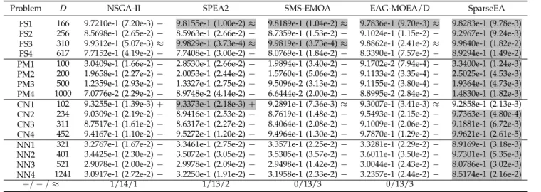
Table III lists the median HV values and interquar-tile ranges obtained by NSGA-II, SPEA2, SMS-EMOA, EAG-MOEA/D, and the proposed SparseEA on FS1– FS4, PM1–PM4, CN1–CN4, and NN1–NN4. It is obvious from the table that SparseEA significantly outperforms the other four MOEAs in terms of HV, having achieved the best performance on all the test instances besides CN1. As a result, a similar trend as in Table I can be observed in Table III, and it is confirmed that the proposed SMOP1–SMOP8 can characterize the sparse MOPs in applications.

Fig. 9 plots the non-dominated solution sets with me-dian HV among 30 runs obtained by the five MOEAs on FS4. Besides, the result obtained by sequential forward selection (SFS) [27] is also shown in the figure, which is a traditional feature selection approach. It can be found that the solutions obtained by NSGA-II, SPEA2, SMS-EMOA, and EAG-MOEA/D are non-dominated with or dominated by those obtained by SFS, whereas the solu-tions obtained by SparseEA can dominate those obtained by SFS and the other four MOEAs. Figs. 10 and 11 plot the results on PM4 and CN4, where the results ob-tained by a traditional pattern mining approach DOFIA [10] and a traditional critical node detection approach SEQ [80] are also shown in the figures. It turns out that the solution sets obtained by SparseEA have better convergence and diversity than those obtained by the traditional approaches and the compared MOEAs.

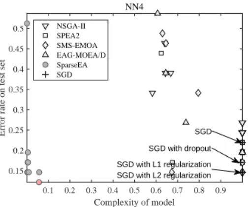
Fig. 12 depicts the results obtained by the five MOEAs on NN4. The result obtained by stochastic gradient descent (SGD) [81] is also shown in the figure, where the learning rate is set to 1, the momentum is set to 0.95, the minibatch size is set to 20, and the number of epochs

(12)

TABLE III

MEDIANHV VALUES ANDINTERQUARTILERANGESOBTAINED BYNSGA-II, SPEA2, SMS-EMOA, EAG-MOEA/D,ANDSPARSEEAON FS1–FS4, PM1–PM4, CN1–CN4,ANDNN1–NN4, WHERE THERESULTS NOTSIGNIFICANTLYWORSE THAN ANYOTHERS AREHIGHLIGHTED.

Problem D NSGA-II SPEA2 SMS-EMOA EAG-MOEA/D SparseEA

FS1 166 9.7210e-1 (7.20e-3)− 9.8155e-1 (1.00e-2)≈ 9.8189e-1 (1.04e-2)≈ 9.7836e-1 (9.70e-3)≈ 9.8283e-1 (9.78e-3) FS2 256 8.5698e-1 (2.65e-2)− 8.5963e-1 (2.66e-2)− 8.7359e-1 (1.53e-2)− 9.1024e-1 (1.15e-2)− 9.2967e-1 (9.24e-3) FS3 310 9.9312e-1 (5.07e-3)≈ 9.9829e-1 (3.73e-4)≈ 9.9819e-1 (3.73e-4)≈ 9.8862e-1 (2.41e-2)≈ 9.9840e-1 (1.82e-2) FS4 617 7.7152e-1 (4.19e-2)− 7.7408e-1 (3.00e-2)− 8.0769e-1 (1.84e-2)− 8.3390e-1 (7.57e-2)− 8.9294e-1 (1.49e-2) PM1 100 3.0409e-1 (1.66e-2)− 2.8530e-1 (2.66e-2)− 1.9894e-1 (3.40e-2)− 9.1702e-2 (7.94e-4)− 3.3400e-1 (1.24e-3) PM2 200 1.9658e-1 (2.27e-2)− 2.0053e-1 (2.44e-2)− 1.5760e-1 (5.06e-2)− 9.1133e-2 (3.35e-4)− 2.5025e-1 (4.53e-3) PM3 500 1.2359e-1 (2.93e-2)− 1.3327e-1 (2.75e-2)− 9.5096e-2 (3.13e-2)− 9.1155e-2 (3.80e-4)− 1.9364e-1 (4.73e-3) PM4 1000 7.0776e-2 (2.29e-2)− 8.9748e-2 (4.14e-2)− 6.6444e-2 (2.00e-2)− 8.8995e-2 (2.84e-2)− 1.4830e-1 (1.82e-3) CN1 102 9.3255e-1 (1.39e-3)+ 9.3373e-1 (2.18e-3)+ 9.2891e-1 (7.36e-3)≈ 9.3007e-1 (3.41e-3)≈ 9.2858e-1 (2.13e-3) CN2 234 9.0309e-1 (2.19e-2)− 8.9416e-1 (2.53e-2)− 8.7619e-1 (1.48e-2)− 9.5493e-1 (2.15e-2)− 9.7363e-1 (4.80e-4) CN3 311 8.7517e-1 (1.61e-2)− 8.6317e-1 (2.27e-2)− 8.4064e-1 (2.08e-2)− 9.1009e-1 (2.06e-2)− 9.1881e-1 (6.72e-3) CN4 452 9.4167e-1 (1.10e-2)− 9.5272e-1 (1.20e-2)− 9.4964e-1 (1.30e-2)− 9.7870e-1 (1.29e-2)− 9.9621e-1 (2.61e-5) NN1 321 3.2767e-1 (1.67e-2)− 3.3461e-1 (2.75e-2)− 3.3571e-1 (2.25e-2)− 3.3281e-1 (2.29e-2)− 8.9169e-1 (3.18e-3) NN2 401 3.4425e-1 (2.30e-2)− 3.5072e-1 (3.05e-2)− 3.5305e-1 (3.57e-2)− 3.6011e-1 (3.50e-2)− 9.7301e-1 (5.35e-3) NN3 521 2.9078e-1 (2.00e-2)− 2.9978e-1 (2.09e-2)− 2.9498e-1 (1.42e-2)− 3.0044e-1 (2.43e-2)− 8.0786e-1 (3.02e-3) NN4 1241 3.0917e-1 (2.72e-2)− 3.2250e-1 (1.91e-2)− 3.1958e-1 (2.33e-2)− 3.2357e-1 (2.44e-2)− 8.5174e-1 (2.16e-2)

+/−/≈ 1/14/1 1/13/2 0/13/3 0/13/3

‘+’, ‘−’ and ‘≈’ indicate that the result is significantly better, significantly worse and statistically similar to that obtained by SparseEA, respectively.

0 0.05 0.1 0.15 0.2 0.25

0.1 0.2 0.3 0.4 0.5 0.6 0.7 0.8 0.9

FS4 NSGA-II SPEA2 SMS-EMOA EAG-MOEA/D SparseEA SFS

Fig. 9. Objective values of the solution sets with median HV among 30 runs obtained by NSGA-II, SPEA2, SMS-EMOA, EAG-MOEA/D, SparseEA, and SFS on FS4. 0 0.2 0.4 0.6 0.8 1 1 - frequency 0 0.2 0.4 0.6 0.8 1 1 - completeness PM4 NSGA-II SPEA2 SMS-EMOA EAG-MOEA/D SparseEA DOFIA

Fig. 10. Objective values of the solution sets with median HV among 30 runs obtained by NSGA-II, SPEA2, SMS-EMOA, EAG-MOEA/D, SparseEA, and DOFIA on PM4.

is set to 25000. Besides, the results obtained by SGD with dropout (dropout rate is set to 0.5) and SGD with L1 and L2 regularizations (penalty parameter is set to 0.1) are

0 0.02 0.04 0.06 0.08 0.1

Ratio of deleted nodes

10-4 10-3 10-2 10-1 100 Pairwise connectivity CN4 NSGA-II SPEA2 SMS-EMOA EAG-MOEA/D SparseEA SEQ

Fig. 11. Objective values of the solution sets with median HV among 30 runs obtained by NSGA-II, SPEA2, SMS-EMOA, EAG-MOEA/D, SparseEA, and SEQ on CN4.

0.1 0.2 0.3 0.4 0.5 0.6 0.7 0.8 0.9 Complexity of model 0 0.05 0.1 0.15 0.2 0.25 0.3 0.35 0.4 0.45

Error rate on training set

NN4 NSGA-II SPEA2 SMS-EMOA EAG-MOEA/D SparseEA SGD SGD with L1 regularization SGD with L2 regularization SGD with dropout SGD

Fig. 12. Objective values of the solution sets with median HV among 30 runs obtained by NSGA-II, SPEA2, SMS-EMOA, EAG-MOEA/D, SparseEA, and SGD on NN4.

also presented. As can be seen from Fig. 12, the networks obtained by SparseEA have the lowest complexities, but their error rates on training set are higher than those

(13)

0.1 0.2 0.3 0.4 0.5 0.6 0.7 0.8 0.9 Complexity of model 0.15 0.2 0.25 0.3 0.35 0.4 0.45 0.5

Error rate on test set

NN4 NSGA-II SPEA2 SMS-EMOA EAG-MOEA/D SparseEA SGD SGD with L1 regularization SGD with L2 regularization SGD with dropout SGD

Fig. 13. The test error rates of the solutions shown in Fig. 12.

Input layer Hidden layer Output layer

Fig. 14. The neural network with the lowest test error rate on NN4 obtained by the proposed SparseEA. This network is so sparse that it contains only 13 weights.

obtained by SGD and some other MOEAs. By contrast, according to the error rates on test set shown in Fig. 13, it can be found that the networks obtained by SparseEA have lower error rates on test set than those obtained by SGD and other MOEAs. Note that the training set consists of 80% samples in the dataset, while the test set consists of the rest 20% samples. As a consequence, the networks obtained by SGD and other MOEAs overfit the training set, whereas the networks obtained by SparseEA can alleviate overfitting. For further observations, Fig. 14 presents the structure of the neural network with the lowest test error rate obtained by SparseEA. It can be seen from the figure that the neural network is so sparse that it contains only 13 weights. To summarize, the proposed SparseEA is more effective than existing MOEAs for sparse MOPs.

VII. CONCLUSIONS

Many MOPs in real-world applications have sparse Pareto optimal solutions, however, such type of MOPs has not been exclusively investigated before, and most work only adopts existing MOEAs to solve them. To fill this gap, this paper has proposed an MOEA for solving large-scale sparse MOPs, called SparseEA. The proposed SparseEA uses a new population initialization strategy and genetic operators to generate sparse solutions, which is empirically verified to be more effective than existing MOEAs for sparse MOPs.

Due to the broad application scenarios of sparse

MOPs, further investigation on this topic is still desir-able. Firstly, it is interesting to combine SparseEA with customized search strategies for solving specific sparse MOPs in applications. Secondly, it is desirable to adopt other environmental selection strategies in SparseEA for solving sparse MOPs with many objectives. Thirdly, since SparseEA evolves the population without consid-ering the interactions between decision variables, it can be enhanced by adopting other strategies like decision variable clustering [30] and Bayesian optimization [36]. Finally, the scores of decision variables can be dynam-ically updated during the evolution to make it more accurate.

REFERENCES

[1] C. A. Coello Coello, G. B. Lamont, and D. A. Van Veldhuizen,

Evolutionary algorithms for solving multi-objective problems. Springer Science & Business Media, 2007.

[2] A. Ponsich, A. L. Jaimes, and C. A. C. Coello, “A survey on multi-objective evolutionary algorithms for the solution of the portfolio optimization problem and other finance and economics appli-cations,” IEEE Transactions on Evolutionary Computation, vol. 17, no. 3, pp. 321–344, 2013.

[3] Y. Zhang, M. Harman, and S. A. Mansouri, “The multi-objective next release problem,” inProceedings of the 9th Annual Conference on Genetic and Evolutionary Computation, 2007, pp. 1129–1137. [4] L. Zhang, H. Pan, Y. Su, X. Zhang, and Y. Niu, “A mixed

representation-based multiobjective evolutionary algorithm for overlapping community detection,” IEEE Transactions on Cyber-netics, vol. 47, no. 9, pp. 2703–2716, 2017.

[5] J. D. Schaffer, “Multiple objective optimization with vector eval-uated genetic algorithms,” in Proceedings of the 1st International Conference on Genetic Algorithms, 1985, pp. 93–100.

[6] A. Zhou, B.-Y. Qu, H. Li, S.-Z. Zhao, P. N. Suganthan, and Q. Zhang, “Multiobjective evolutionary algorithms: A survey of the state of the art,”Swarm and Evolutionary Computation, vol. 1, no. 1, pp. 32–49, 2011.

[7] M. Dash and H. Liu, “Feature selection for classification,” Intelli-gent data analysis, vol. 1, no. 3, pp. 131–156, 1997.

[8] B. Xue, M. Zhang, and W. N. Browne, “Particle swarm opti-mization for feature selection in classification: A multi-objective approach,” IEEE Transactions on Cybernetics, vol. 43, no. 6, pp. 1656–1671, 2013.

[9] C. Qian, Y. Yu, and Z.-H. Zhou, “Subset selection by Pareto op-timization,” inAdvances in Neural Information Processing Systems, 2015, pp. 1774–1782.

[10] L. Tang, L. Zhang, P. Luo, and M. Wang, “Incorporating oc-cupancy into frequent pattern mining for high quality pattern recommendation,” in Proceedings of the 21st ACM International Conference on Information and Knowledge Management, 2012, pp. 75– 84.

[11] M. Lalou, M. A. Tahraoui, and H. Kheddouci, “The critical node detection problem in networks: A survey,”Computer Science Review, vol. 28, pp. 92–117, 2018.

[12] J. E. Fieldsend and S. Singh, “Pareto evolutionary neural net-works,”IEEE Transactions on Neural Networks, vol. 16, no. 2, pp. 338–354, 2005.

[13] H. Li, Q. Zhang, J. Deng, and Z.-B. Xu, “A preference-based multiobjective evolutionary approach for sparse optimization,”

IEEE Transactions on Neural Networks and Learning Systems, vol. 29, no. 5, pp. 1716–1731, 2018.

[14] Y. Jin, T. Okabe, and B. Sendhoff, “Neural network regularization and ensembling using multi-objective evolutionary algorithms,” inProceedings of the 2004 IEEE Congress on Evolutionary Computa-tion, 2004, pp. 1–8.

[15] R. Tibshirani, “Regression shrinkage and selection via the lasso,”

Journal of the Royal Statistical Society. Series B (Methodology), vol. 58, no. 1, pp. 267–288, 1996.

[16] B. A. Olshausen and D. J. Field, “Sparse coding with an over-complete basis set: A strategy employed by V1?”Vision Research, vol. 37, no. 23, pp. 3311–3325, 1997.