Selection Methods and Diversity Preservation in
Many-Objective Evolutionary Algorithms
Luis Mart´ı
1Eduardo Segredo
2,3Nayat S´anchez-Pi
4Emma Hart
21. Institute of Computing, Universidade Federal Fluminense, Niter´oi (RJ) Brazil. 2. School of Computing, Edinburgh Napier University, Edinburgh, Scotland, UK 3. Dpto. Ingenier´ıa Inform´atica y de Sistemas, Universidad de La Laguna, San
Crist´obal de La Laguna, Spain.
4. DICC/IME, Rio de Janeiro State University, Rio de Janeiro (RJ) Brazil.
Abstract
Purpose– One of the main components of multi-objective, and therefore,
many-objective evolutionary algorithms is the selection mechanism. It is responsible for performing two main tasks simultaneously. First, it has to promote convergence by selecting solutions which are as close as possible to the Pareto optimal set. And second, it has to promote diversity in the solution set provided. In the current work, an exhaustive study that involves the comparison of several selection mechanisms with different features is performed. Particularly, Pareto-based and indicator-based selection schemes, which belong to well-known multi-objective optimisers, are considered.
Design/methodology/approach– Each of those mechanisms is incorporated into
a common multi-objective evolutionary algorithm framework. The main goal of the study is to measure the diversity preserved by each of those selection meth-ods when addressing many-objective optimisation problems. The Walking Fish Group (WFG) test suite, a set of optimisation problems with a scalable number of objective functions, is taken into account to perform the experimental evaluation.
Findings– The computational results highlight that the the reference-point-based
selection scheme of the Non-dominated Sorting Genetic Algorithm III (NSGA-III) and a modified version of the Non-dominated Sorting Genetic Algorithm II (NSGA-II), where the crowding distance is replaced by the Euclidean distance, are able to provide the best performance, not only in terms of diversity preservation, but also in terms of convergence.
Originality/value– The performance provided by the use of the Euclidean
dis-tance as part of the selection scheme indicates this is a promising line of research and, to the best of our knowledge, it has not been investigated yet.
Keywords:multi-objective evolutionary algorithm; many-objective optimisation; selection
1
Introduction
Multi-objective optimisation is aimed to deal with optimisation problems defined by a set of objective functions, which must be optimised in a simultaneous way. Those objective functions are conflicting one to each other. In the related literature, these types of problems are referred to asMulti-objective Optimisation Problems(MOPs). MOPs can be found on a significant number of real-world applications in different fields, such as aircraft engineering (Reynoso Meza et al. 2017), engine design (Patel et al. 2017), renewable energies (Tanwar & Khatod 2017), and controller design (Freire et al. 2017), among many others.Many-objective Optimisation Problems(MaOPs) are those MOPs where more than three objective functions have to be optimised (Ishibuchi et al. 2008). ThePareto optimal frontorPareto optimal setare the terms used to refer to the solution of a MOP, and therefore, a MaOP. The Pareto optimal front consists of a set of trade-off points in the space of the objective functions.
At this point, we should note that the Pareto optimal set can be obtained by means of mathematical programming approaches, in case the MOP we are dealing with satisfies several requirements, for instance, convexity of the feasible set, and linearity or convex-ity of the objective functions (Branke et al. 2008). Nevertheless, in general, providing the solution of a MOP is anN P-complete problem (B¨ack 1996). Bearing the above in mind, exact algorithmic approaches are not applicable, and consequently, a wide range of heuristic and meta-heuristic techniques has been proposed in the related literature to deal with MOPs. Multi-objective Evolutionary Algorithms(MOEAs) (Coello Coello et al. 2007) are one of the most popular algorithmic schemes to address MOPs in a suc-cessful way. A large number ofMulti-objective Evolutionary Algorithms(MOEAs) has been designed to tackle MOPs (Coello Coello et al. 2007), such as theNon-dominated Sorting Genetic Algorithm II(NSGA-II) (Deb et al. 2002), theStrength Pareto Evo-lutionary Algorithm 2(SPEA2) (Zitzler et al. 2001), theMulti-objective Evolutionary Algorithm based on Decomposition(MOEA/D) (Zhang & Li 2007), theGrid-based Evolutionary Algorithm(GrEA) (Yang et al. 2013) and theIndicator-based Evolution-ary Algorithm(IBEA) (Zitzler & K¨unzli 2004), among others.
The approach used to select the individuals that will survive for the next generation of a MOEA is referred to as the selection scheme, and is one of the most important components in these types of algorithms. Particularly, the selection scheme is respon-sible for balancing the convergence and the diversity of the solution set provided. One of the most frequently used selection mechanisms is based on Pareto optimality con-cepts. Pareto-based selection usually takes into account two independent selection criteria (Liu et al. 2017). First of all, individuals are ranked by applying Pareto opti-mality such that the non-dominated individuals are assigned to a better rank. After-wards, in order to differentiate individuals that have been assigned to the same rank, a diversity-based criterion is used. Pareto-based selection has proven to be one of the most successful selection methods to deal with a large number of MOPs. When ad-dressing MaOPs, however, the application of Pareto-based MOEAs is not appropriate. In the case of dealing with MaOPs, the larger the number of objective functions, the higher the number of non-dominated solutions. In this scenario, the Pareto-based se-lection approach becomes inaccurate when ranking individuals, and consequently, the selection pressure of the whole MOEA decreases. This lack of convergence causes that
the solution set provided is not close enough to the Pareto optimal set.
With the aim of improving the performance of Pareto-based MOEAs when dealing with MaOPs, three options have been explored mainly (Liu et al. 2017). The first option is based on providing new dominance definitions that are able to increase the selection pressure of the MOEA. Examples would be thedominance area control(Sato et al. 2011) and theL-optimality(Zou et al. 2008). The improvement or replacement of the diversity-based selection criterion is the second option. An example of the above is the novel diversity preserving strategy based on dynamic crowding distance proposed by Yang et al. (2017). The third option consists of providing MOEAs that do not make use of Pareto-based selection (Liu et al. 2017):decomposition-basedMOEAs,grid-based
MOEAs andindicator-basedMOEAs. Finally, the order in which the convergence and diversity-based criteria are considered to select individuals has also been analysed. For instance, Jiang & Yang (2016) proposed a novel MOEA calledDiversity-first Based Evolutionary Algorithm(DBEA) that considers diversity, rather than convergence, as the first criterion in the selection mechanism. DBEA demonstrated to attain a better performance for a significant number of the functions tested in comparison to the well-known NSGA-III.
A very important research question to be answered and that has arisen as a very active research field is how to measure the performance of MOEAs properly (Li et al. 2014). A wide range of quality indicators, such as thehypervolume indicator(Zitzler et al. 1999) and theDiversity Comparison Indicator(Li et al. 2014), among others, have been proposed for measuring either convergence or diversity or both of them. In the current paper, we focus on quality indicators specifically designed for measuring the diversity of a solution set.
Considering the above discussion, in this work we carry out an exhaustive compar-ison of different selection mechanisms with different features highlighting the impact they have on the diversity preserved by MOEAs when addressing MaOPs. For doing that, several selection methods belonging to well-known MOEAs are incorporated into a common multi-objective evolutionary algorithm framework and applied to a set of MaOPs with a scalable number of objective functions called theWalking Fish Group
(WFG) test suite (Huband et al. 2005). Different quality indicators are used to assess the performance of the algorithmic schemes tested. At this point, it is worth mentioning that an initial study regarding the above issue was performed by the authors in Mart´ı et al. (2017). The main contribution of the current work with respect to that previous one is we provide a significant extension of the experimental evaluation by considering a larger number of objective functions, which increases the complexity of the MaOPs addressed noticeably. Furthermore, we also provide a comprehensive statistical analy-sis involving the different selection mechanisms tested.
The rest of the paper is organised as follows. Section 2 briefly describes all the foundations related to the work carried out in this paper, including the formal definition of a MOP, the particular MOEAs we have taken into consideration for our analyses, as well as their corresponding selection mechanisms. The particular quality indicators selected to measure the diversity of the solution sets attained by those MOEAs are also depicted. Afterwards, the experimental evaluation carried out, as well as the results obtained, are commented in Section 3. Finally, some conclusions and lines of further research are shared in Section 4.
2
Foundations
AMulti-objective Optimisation Problem(MOP) can be defined as the problem in which a set ofobjective functionsf1(x), . . . , fM(x)should be jointly optimised1;
min F(x) =hf1(x), . . . , fM(x)i; x∈ S; (1)
whereS ⊆Rnis known as thefeasible setand can be expressed as a set of restric-tions over thedecision set, in our case,Rn. Theimage setofSproduced by function vectorF(·), i.e.,O ⊆RM is called thefeasible objective setorcriterion set. The so-lution to these types of problems is a set of trade-off points. The optimality of a given solution can be defined in terms of the Pareto dominance relation.
Definition 1(Pareto dominance relation). For the optimisation problem specified in
(1) and havingx,y∈ S,xis said to dominatey(expressed asx≺y) iff∀fj=1,...,M,
fj(x)≤fj(y)and∃fi=1,...,M such thatfi(x)< fi(y).
Definition 2(Non-dominated subset). In problem (1) and having the setA ⊆ S,A,ˆ
the non-dominated subset ofA, is defined as
b
A={x∈ A |6 ∃x0 ∈ A:x0≺x}.
The solution of (1) isSˆ, thenon-dominated subsetofS.Sˆis known as theefficient setor Pareto-optimal set (Branke et al. 2008). The Pareto-optimal front, Oˆ, is the image ofSˆ in the feasible objective set.
If problem (1) has certain characteristics, e. g., linearity or convexity of the objec-tive functions or convexity ofS, the efficient set can be determined by mathematical programming approaches (Branke et al. 2008). However, in the general case, finding the solution of (1) is anNP–complete problem (B¨ack 1996). In this case, heuristic and/or meta-heuristic methods, such asEvolutionary Algorithms(EAs) (Coello Coello et al. 2007), have arisen as one of the most popular techniques for successfully address-ing MOPs.
A wide range ofMulti-objective Evolutionary Algorithms(MOEAs) has been pro-posed in the related literature to tackle MOPs successfully (Coello Coello et al. 2007). A significant number of those MOEAs incorporates a Pareto-based selection scheme. Individuals are ranked by applying Pareto optimality, and the non-dominated ones are selected to survive with a higher probability. Nevertheless, it has been demon-strated that Pareto-based selection is not suitable for MOPs with more than three ob-jective functions, which are usually known asMany-objective Optimisation Problems
(MaOPs) (Ishibuchi et al. 2008).
Several are the challenges that arise when trying to deal with MaOPs, for instance, an exponential increase of non-dominated individuals when the number of objective functions rises, which deteriorates the selection pressure of the whole optimiser, as well as issues related to the visualisation of the Pareto front approximations obtained, among others.
2.1
Assessing the diversity of a Pareto set approximation
Several are the quality indicators that have been proposed for measuring different as-pects related to the shape of a Pareto set approximation, mainly, convergence, spread and uniformity2. From the above three aspects, we note that both spread and
unifor-mity, which are closely related, determine the diversity of a Pareto set approximation. This section is devoted to briefly describe some well-known quality indicators that we apply herein as performance metrics. We have selected theDiversity Measure (Sec-tion 2.1.1) and theDiversity Comparison Indicator(Section 2.1.2) for our analyses be-cause they focus on diversity according to the taxonomy proposed by Li et al. (2014). Thehypervolume (Section 2.1.3) has also been chosen, since it not only focuses on diversity but also on convergence, and is one of the most frequently used indicators to assess the performance of MOEAs.
2.1.1 Diversity Measure (DM)
TheDiversity Measure(DM) was proposed to calculate the amount of diversity of a Pareto set approximation (Deb & Jain 2002). For doing that, it considers a reference set. The solutions belonging to both the reference set and the approximation are assigned to different grids or divisions of a hyperplane withM −1dimensions, withM being the number of objectives of the problem at hand. Those divisions are called hyper-boxes. The number of solutions assigned to a particular hyper-box, as well as the number of solutions assigned to its neighbour hyper-boxes, are used to evaluate that hyper-box. The larger the number of hyper-boxes containing solutions that belong to both the reference set and the approximation, the larger the indicator value, which is in the range[0,1]. Bearing the above in mind, the value one indicates that maximum diversity has been reached. In this case, every solution of the approximation has been assigned to a hyper-box containing solutions of the reference set. At the same time, a DM value equal to zero means that the Pareto front approximation is not diverse at all, since no point belonging to the former has been assigned to a hyper-box which contains solutions of the reference set. According to Li et al. (2014), DM has several disadvantages when dealing with MaOPs:
1. A reference set with solutions uniformly distributed in the Pareto front is
required. Providing a reference set is an arduous task, even more in the case of many-objective optimisation. Furthermore, the number of solutions in the said reference set should be approximately equal to the number of solutions in the Pareto set approximation.
2. A distribution estimation has to be calculated for each hyper-box. There exist
rM−1hyper-boxes, withrbeing the number of divisions in every dimension.
3. A value function has to be computed for each neighbour hyper-boxwhen
es-timating the distribution of a given hyper-box. A particular hyper-box has3M−1
neighbours. As a result, computing that value function may be challenging in the case of dealing with MaOPs.
2Since the shape of Pareto set approximations are taken into consideration, quality indicators are usually
4. An inaccurate value of the approximation diversity could be provided, since the Manhattan distance is taken into account, rather than the Euclidean distance.
2.1.2 Diversity Comparison Indicator (DCI)
The great majority of those indicators aimed to measure the amount of diversity of a Pareto set approximation are not suitable for problems with a large number of objective functions (Li et al. 2014). TheDiversity Comparison Indicator(DCI) was specifically proposed to measure the diversity of many-objective Pareto front approximations (Li et al. 2014). It tries to solve the aforementioned drawbacks that arise when metrics, such as DM, are applied to assess the performance of MaOPs. DCI takes different Pareto front approximations and evaluates their relative contribution to diversity instead of calculating the absolute contribution of a unique Pareto set approximation.
It considers a grid environment, which consists of a set of hyper-boxes, where the solutions belonging to the approximations are distributed. Only nonempty hyper-boxes, i.e., hyper-boxes where one or more non-dominated solutions belonging to the mixed set of approximations have been assigned, are taken into account by DCI to calculate the contribution of each approximation. Hence, given a particular approx-imation, if its solutions are assigned or are close to the majority of the nonempty hyper-boxes, then its contribution to diversity will be significant in comparison to the contribution of the other Pareto set approximations. If its solutions are not assigned or are far away from most of those nonempty hyper-boxes, however, then its contri-bution to diversity will be poor. The contricontri-bution of each Pareto set approximation to each nonempty hyper-box has thus to be calculated. That contribution is measured in terms of the grid distance between the Pareto set approximation and the hyper-box considered.
The grid distanceGDbetween two hyper-boxesh1andh2in the grid is computed as it is shown by (2), withhk
1 andhk2giving the coordinates ofh1 andh2in thek-th
objective, respectively. It can be observed that the Euclidean distance is considered by DCI. GD(h1, h2) = v u u t M X k=1 (hk 1−hk2)2 (2)
The grid distanceDbetween an approximationP and a hyper-boxhis the mini-mum grid distance betweenhand any other hyper-box, referred to asG(p), containing at least one solutionpbelonging toP:
D(P, h) = min
p∈P{GD(h, G(p))} (3)
Therefore, the contributionCD of an approximationP to a hyper-boxhcan be computed as follows: CD(P, h) = ( 1−D(P,h)2 M+1 , D(P, h)< √ M + 1 0, D(P, h)≥√M + 1 (4)
Finally, considering a Pareto front approximationP, its DCI value can be calculated as it is shown by (5), where the number of nonempty hyper-boxes is given byS.
DCI(P) = 1 S S X i=1 CD(P, hi) (5)
The main advantages of this indicator are the following ones:
1. It does not require a reference set, in opposition to other indicators, such as
DM.
2. It cannot only be applied to compare two Pareto front approximations, but
several of them.
3. The execution time of DCI, which belongs toO(M(LN)2), is independent
of the number of hyper-boxes. Lis the number of Pareto set approximations
andN is the number of solutions in those approximations.
2.1.3 Hypervolume indicator
The hypervolume indicator,Ihyp(A), (Zitzler et al. 1999, 2007, Knowles 2002, Knowles
et al. 2006) computes the volume of the regionH delimited by a given set of points,
A, and a set of reference points,N, as it is shown by (6). Therefore, larger values of the indicator will correspond to better solutions.
Ihyp(A) = volume [ ∀a∈A;∀n∈N hypercube(a,n) (6)
The hypervolume indicator is also known as theSmetric or the Lebesgue measure. It has many attractive features that have favoured its application and popularity. In particular, it is the only indicator that has the properties of a metric and the only one to be strictly Pareto monotonic (Fleischer 2003, Zitzler et al. 2003). Because of these properties, this indicator has been used not only for performance assessment but also as part of some MOEAs (see Section 2.4 for further information).
To measure the absolute performance of an algorithm, the reference points should benadir pointsideally. These points are the worst elements ofOor, in other words, the elements ofOthat do not dominate any other element. To contrast the relative performance of two sets of solutions, though, one can be used as the reference set. These matters were further detailed by Zitzler et al. (2002) and Knowles et al. (2006).
HavingN, the computation of the indicator is a non-trivial problem. Indeed, its determination is known to be computationally intensive, thus rendering it unsuitable for MaOPs. As a result, a significant amount of research has focused on improving the computational complexity of this indicator (While et al. 2006, 2005, Fonseca et al. 2006, Beume 2009). The exact computation of the algorithm has been shown to be
#P-hard (Bringmann & Friedrich 2010) in the number of objectives. These types of problems are the analogous ofNPfor counting problems (Papadimitriou 1994). There-fore, all algorithms calculating the hypervolume must have an exponential run-time
with regard to the number of objectives if P 6= N P, something that seems to be true (Deolalikar 2010).
According to the most recent results, the indicator is known to be O(nlogn+
nM/2)(Beume 2009) for more than three objectives (M >3);O(nlogn)for M = 2,3(Fonseca et al. 2006). One alternative to circumvent the complexity hurdle is to apply estimation algorithms capable of yielding an approximation of the indicator at a more convenient temporal cost. Monte Carlo sampling(Bader & Zitzler 2008) and
k-greedy strategy(Zitzler et al. 2010) have been applied successfully.
The hypervolume can also be used to measure the progress of an algorithm as the evolution proceeds. For doing that, the relative formulation of the binary hypervolume indicator (Knowles et al. 2006) is usually considered:
Ihyp(A,B) =Ihyp(A)−Ihyp(B). (7) SubstitutingAandBby the non-dominated elements of the current and the previ-ous iteration,PF∗
t andPF∗t−1, respectively, the indicator can be expressed as: Ihyp(t) =Ihyp(PF∗t)−Ihyp PF∗t−1
. (8)
2.2
MOEA selection
A wide variety of algorithms, like the Non-dominated Sorting Genetic Algorithm II
(NSGA-II) (Deb et al. 2002), which is described at Section 2.3, or theimproved Strength Pareto Evolutionary Algorithm(SPEA2) (Zitzler et al. 2001), have been designed by incorporating Pareto optimality as the main selection criterion. Nevertheless, Pareto-based selection is not suitable for many-objective optimisation. One of the main op-tions to increase the performance of Pareto-based MOEAs when dealing with MaOPs is to modify or replace the diversity-based criterion present at their selection scheme. This is the choice addressed, for instance, by theNon-dominated Sorting Genetic Al-gorithm III(NSGA-III) (Jain & Deb 2014).
A different class of MOEAs are those incorporating a quality or performance in-dicator, like the hypervolume (Zitzler et al. 1999) or the R2 indicator (Hansen & Jaszkiewicz 1998), into the selection mechanism. These quality indicators are usu-ally designed for assessing either convergence or diversity or both of them. Individuals are thus selected depending on their contribution to convergence and/or diversity of the solution set they belong to. That contribution is measured by the particular quality indicator applied. The indicator-based MOEAs we have selected for our analyses will be depicted at Section 2.4.
2.3
Pareto-based selection with crowding distance: NSGA-II
NSGA-II is an improvement over the originalNon-dominated Sorting Genetic Algo-rithm(NSGA) (Srinivas & Deb 1994). NSGA-II incorporates two key operations: fast non-dominated sorting of the population and crowding distance computation with the aim of promoting diversity in the population.
The crowding distance considers the size of the largest cuboid enclosing each indi-vidual without including any other member of the population. This feature is used to keep diversity in the population, where solutions belonging to the same rank and with a higher crowding distance are assigned a better fitness than those with a lower crowding distance, avoiding the use of the fitness sharing factor.
2.4
Indicator-based selection
This section is devoted to describe the particular indicator-based MOEAs we have se-lected in order to carry out our study. Particularly, we have sese-lected two algorithms that incorporate two well-known quality indicators. The first one makes use of the hypervolume indicator, while the second one applies the R2 indicator.
2.4.1 SMS-EMOA
TheS-metric Selection Evolutionary Multi-objective Optimisation Algorithm (SMS-EMOA), which was proposed by Beume et al. (2007), is a steady-state algorithm, i.e., only one offspring is produced and only one individual has to be removed from the population at every generation. The hypervolume is not computed exactly. Instead, the
k-greedy strategy is employed. These decisions were made in the hope of tackling the high computational demands of computing the hypervolume.
The key element of SMS-EMOA is the method for determining which element of the population will be replaced by the offspring. This is done by applying a non-domination ranking. From the individuals that are dominated by the rest of the pop-ulation, one individual is selected such that it makes the minimum contribution to the hypervolume considering the whole set. Then, this individual is removed from the pop-ulation and substituted by a new individual generated by the usual variation operators. It may happen that there exists a unique non-dominated front (where all individuals in the population are non-dominated). In this particular case, the individual with the lowest contribution to the total hypervolume is selected to be replaced.
2.4.2 R2-EMOA
The R2-EMOA algorithm was originally proposed by Trautmann et al. (2013) and was analysed in depth by Brockhoff et al. (2015). As in the case of SMS-EMOA, R2-EMOA is a steady-state approach, but it incorporates the R2 indicator (Hansen & Jaszkiewicz 1998) as the secondary criterion for guiding the selection. The individual
a∗belonging to the worst rankRhand allowing the smallest R2 indicator value
asso-ciated to the remaining individuals of that worst rank to be obtained, is selected to be replaced by the offspring. The aforementioned procedure is depicted by (9). Parame-tersr∗andΛare the utopian point and the set of weight vectors, respectively, which allow preferences of a decision maker to be incorporated into R2-EMOA (Trautmann et al. 2013).
We note that the R2 indicator, as the hypervolume, assess the main three features that a Pareto front approximation should fulfil: convergence, spread and uniformity. The R2 indicator, however, presents two main differences with respect to the hyper-volume. First, the computation of the hypervolume, which takes exponential time in the number of objectives3is avoided. Second, it may avoid the biased behaviour of the hypervolume indicator regarding the solution sets provided, which are usually focused on the knee area of the Pareto front. This is due to the potential incorporation of pref-erences of a decision maker. Similarly, it was shown that, in the bi-objective case, the R2 indicator presents an even more biased behaviour than the hypervolume (Brockhoff et al. 2015).
2.5
Reference-point-based selection: NSGA-III
Another promising line for tackling MaOPs comes from the reference-point-based many-objective version of the II, referred to as III. Similarly to NSGA-II, NSGA-III employs the Pareto non-dominated sorting to partition the population into a number of fronts. In the last front however, rather than using the crowding distance to determine the surviving individuals, a novel niche-preservation operator is applied.
This niche-preservation operator relies on reference points organised in a hyper-plane in order to promote a diverse population. As a result, solutions associated with a smaller number of crowded reference points are more likely to be selected. Finally, we note that a sophisticated normalisation scheme is incorporated into the NSGA-III, which is aimed to effectively handle objective functions of different scales.
3
Experimental results
Theleitmotivof this work is to study the impact that different selection methods have on population diversity when dealing with MaOPs. A shared MOEA framework was used to analyse the selection methods considered under the same experimental conditions. The said framework provided a testing ground common to all approaches, and as a re-sult, we were able to solely focus on the topic of interest. The shared MOEA is similar to other previously proposed algorithms and falls into the(µ+λ)evolutionary strategy scheme. The algorithm is summarised in Fig. 1 as the procedureshared moea( ). It starts with an initial random population,P0, ofµindividuals. After that, at every
iteration,t, an offspring population with λindividuals, Poff, is created by applying
the variation operators inapply variation( )on the current population,Pt.
Sub-sequently, the bestµindividuals are kept for the next generation populationPt+1by
applying a given selection function,sel func(), which is specified as a parameter. Once the stopping criterion is satisfied, the non-dominated subset ofPtis returned.
We note that for our analyses we considered the selection schemes of the following MOEAs, which were introduced at Section 2.2: NSGA-II, NSGA-III, SMS-EMOA, R2-EMOA and a modified version of NSGA-II, where the Euclidean distance substi-tutes the crowding distance in the selection mechanism.
3In the case of dealing with two or three objectives, efficient multi-objective optimisers based on the
functionshared moea(sel func, µ, λ)
.sel func, selection function to be used.
. µandλ, population and offspring sizes.
t←0;P0←random population(µ).
whilestopping criterion not metdo
Poff←apply variation(Pt, λ).
Pt+1←sel func(Pt∪ Poff, µ).
t←t+ 1.
returnnon dom set(Pt+1), final non-dominated set.
Figure 1: Algorithmic representation of the shared MOEA framework.
Table 1: Parameterisation of the different algorithmic approaches
Parameter Value Parameter Value
Number of variables (n) 30 Population size (µ=λ) 50×10M3
Number of objectives (M) 3,6,9,12,15 Simulated Binary Crossover pmate= 0.8;η= 20.0
Stopping criterion 103+M3 evals. Polynomial Mutation pmut=n1;η= 20.0
We chose the WFG multi-objective problem toolkit (Huband et al. 2006) as the benchmark suite. It describes nine complex problems, referred to as WFG1–WFG9, that test whether the optimisation algorithms are capable of handling different chal-lenges, like separability, multi-modality and deceptive local optima, among others. WFG1 is a separable and uni-modal problem with a mixed (concave and convex) Pareto-optimal front. WFG2 has a concave discontinuous Pareto-optimal front and is separable with a combination of uni-modal and multi-modal objective functions. WFG3 is a non-separable uni-modal problem with a linear degenerate Pareto-optimal front. WFG4 is a separable and strongly multi-modal problem that, like the remaining problems, has a concave Pareto-optimal front. This front lies on the first orthant of a skewed hyper-sphere located at the origin. WFG5 is also a separable problem but it has a set of deceptive locally optimal fronts. This feature is meant to evaluate the capacity of the optimisers to avoid getting trapped in local optima. The next problem, WFG6, is a separable problem without the strong multi-modality of WFG4. The remaining three problems have the added difficulty of having a parameter-based bias. WFG7 is uni-modal and separable, like WFG4 and WFG6. WFG8 is a non-separable problem while WFG9 is non-separable, multi-modal and has deceptive local optima.
Each problem was addressed with M = 3,6,9,12,15 objective functions. At the same time, the number of function evaluations was used as the stopping criterion. Particularly, executions were stopped once103+M
3 function evaluations were carried
out, thus performing longer runs for those problems with a higher number of objective functions. The population size of the different approaches was fixed by considering the number of objective functions of the problem at hand as well, i.e. ,µ=λ= 50×10M3.
For all cases, we ran all experiment instances 50 times4. The remaining parameters
0 0.05 0.1 0.15 M = 3 WFG1 WFG2 WFG3 WFG4 WFG5 WFG6 WFG7 WFG8 WFG9 0 0.1 0.2 M = 6 0 0.5 M = 9 0 1 2 M = 12 NSGA-II NSGA-III SMS-EMO A R2-EMO A Euclidean 5 10 M = 15 NSGA-II NSGA-III SMS-EMO A R2-EMO A
Euclidean NSGA-II NSGA-III
SMS-EMO
A
R2-EMO
A
Euclidean NSGA-II NSGA-III
SMS-EMO
A
R2-EMO
A
Euclidean NSGA-II NSGA-III
SMS-EMO
A
R2-EMO
A
Euclidean NSGA-II NSGA-III
SMS-EMO
A
R2-EMO
A
Euclidean NSGA-II NSGA-III
SMS-EMO
A
R2-EMO
A
Euclidean NSGA-II NSGA-III
SMS-EMO
A
R2-EMO
A
Euclidean NSGA-II NSGA-III
SMS-EMO
A
R2-EMO
A
Euclidean
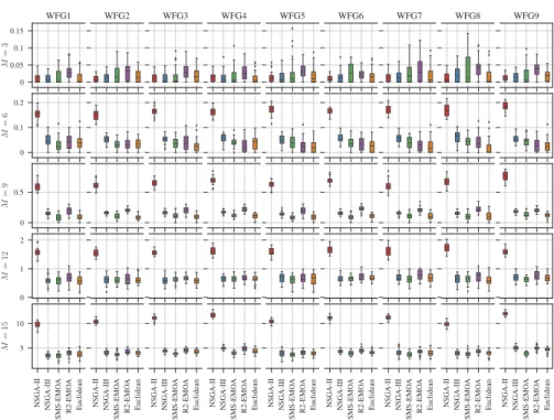
Figure 2: Box plots of the hypervolume values obtained after executing the algorithms on each problem and number of objectives (the lower the values the better).
were fixed as it is shown in Table 1. Finally, the diversity of the resulting solution sets was computed using the hypervolume, DCI and DM indicators, which were described at Section 2.1. As we previously mentioned, the hypervolume indicator is able to capture both convergence of the approximation and its diversity, while both DCI and DM are meant for assessing diversity only.
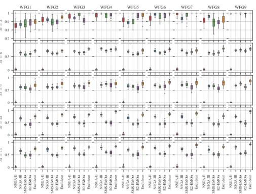
These results are summarised as box plots in Figs. 2, 3 and 4 for the values of hy-pervolume, DCI and DM, respectively. It is particularly interesting that the selection mechanism of NSGA-III, as well as the application of the Euclidean distance rather than the crowding distance by NSGA-II, consistently yielded better results as the num-ber of objective functions grew.
Although illustrative, box plots can not be used to reach a definitive conclusion. That is why statistical hypothesis tests are called for. In our case, for each prob-lem/number of objective functions combination, we performed a Kruskal–Wallis test (Kruskal & Wallis 1952) with the indicator values achieved by each algorithm. In this context, the null hypothesis of this test is that all algorithms are equally capable of solving the problem. If the null hypothesis was rejected, which was actually the case in all instances of the experiment, the Conover–Inman procedure (Conover 1999) was applied in a pairwise manner to determine whether a particular algorithm attained
0.6 0.8 1 M = 3 WFG1 WFG2 WFG3 WFG4 WFG5 WFG6 WFG7 WFG8 WFG9 0 0.5 M = 6 0 0.5 1 M = 9 0 0.5 M = 12 NSGA-II NSGA-III SMS-EMO A R2-EMO A Euclidean 0 0.5 M = 15 NSGA-II NSGA-III SMS-EMO A R2-EMO A
Euclidean NSGA-II NSGA-III
SMS-EMO
A
R2-EMO
A
Euclidean NSGA-II NSGA-III
SMS-EMO
A
R2-EMO
A
Euclidean NSGA-II NSGA-III
SMS-EMO
A
R2-EMO
A
Euclidean NSGA-II NSGA-III
SMS-EMO
A
R2-EMO
A
Euclidean NSGA-II NSGA-III
SMS-EMO
A
R2-EMO
A
Euclidean NSGA-II NSGA-III
SMS-EMO
A
R2-EMO
A
Euclidean NSGA-II NSGA-III
SMS-EMO
A
R2-EMO
A
Euclidean
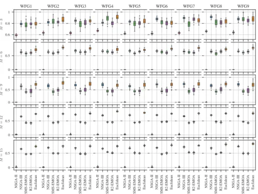
Figure 3: Box plots of the diversity comparison indicator (DCI) obtained after exe-cuting the experiment runs on each problem and number of objectives (the higher the values the better).
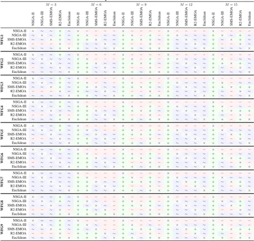
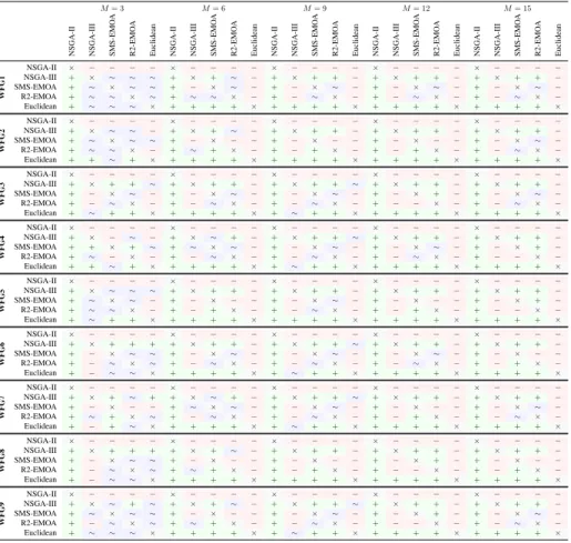
ter results than another. A significance levelα= 0.05, corrected using the Dunn- ˇSid´ak correction, was taken into consideration. The results of these tests are presented in Ta-ble 2 for the hypervolume, TaTa-ble 3 for DCI and TaTa-ble 4 for DM, respectively. In them, it can be verified the results observed in the box plots. In particular the Euclidean and NSGA-III selection methods managed to yield substantially better results.
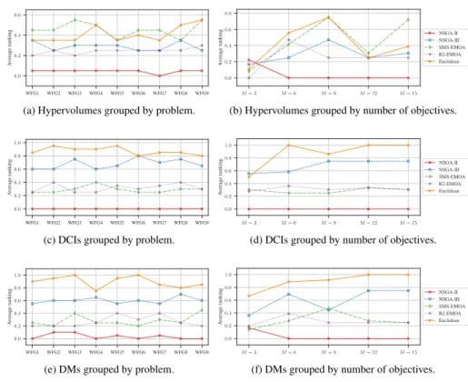
In spite of the effort made to make as illustrative as possible those tables, it is relatively hard to reach a conclusive assessment of the results. To further facilitate the understanding of the results, we decided to adopt a more integrative representation like the one proposed by Bader (2010). This representation groups, either by problem or by number of objectives, the results provided by the different algorithms. It does so by computing the number of times a given algorithm was statistically better than the remaining ones. That is, for a given set of algorithms A1,. . . ,AK, a set ofP test
problem instancesΦ1,m,. . . ,ΦP,m, configured withmobjectives, the functionδ(·)is
defined as
δ(Ai, Aj,Φp,m) =
1 ifAiAjsolvingΦp,m
0 in other case , (10)
where the relationAi Ajdefines ifAiis significantly better thanAjwhen solving
0.7 0.8 0.9 1 M = 3 WFG1 WFG2 WFG3 WFG4 WFG5 WFG6 WFG7 WFG8 WFG9 0 0.5 M = 6 0 0.5 1 M = 9 0 0.5 1 M = 12 NSGA-II NSGA-III SMS-EMO A R2-EMO A Euclidean 0 0.5 1 M = 15 NSGA-II NSGA-III SMS-EMO A R2-EMO A
Euclidean NSGA-II NSGA-III
SMS-EMO
A
R2-EMO
A
Euclidean NSGA-II NSGA-III
SMS-EMO
A
R2-EMO
A
Euclidean NSGA-II NSGA-III
SMS-EMO
A
R2-EMO
A
Euclidean NSGA-II NSGA-III
SMS-EMO
A
R2-EMO
A
Euclidean NSGA-II NSGA-III
SMS-EMO
A
R2-EMO
A
Euclidean NSGA-II NSGA-III
SMS-EMO
A
R2-EMO
A
Euclidean NSGA-II NSGA-III
SMS-EMO
A
R2-EMO
A
Euclidean
Figure 4: Box plots of the diversity metric (DM) obtained after executing the experi-ment runs on each problem and number of objectives (the higher the values the better).
Relying onδ(·), the performance indexPp,m(Ai)of a given algorithmAiwhen solving
Φp,mis then computed as Pp,m(Ai) = K X j=1;j6=i δ(Ai, Aj,Φp,m). (11)
This index intends to summarise the performance of each algorithm with regard to its peers.
Fig. 5 exhibit the results computing the performance indexes grouped by problems and dimensions. Two groups of results are shown. On one hand, the mean performance indexes yielded by each algorithm when solving each problem in all of its configured objective dimensions, ¯ Pp(Ai) = 1 |M| X m∈M Pp,m(Ai). (12)
and, on the other hand, the mean values of the index grouped by each feasible objective set dimension, ¯ Pm(Ai) = 1 P P X p=1 Pp,m(Ai), (13)
WFG1 WFG2 WFG3 WFG4 WFG5 WFG6 WFG7 WFG8 WFG9 0.0 0.2 0.4 0.6 A v erage ranking
(a) Hypervolumes grouped by problem.
M= 3 M= 6 M= 9 M= 12 M= 15 0.0 0.2 0.4 0.6 0.8 A v erage ranking NSGA-II NSGA-III SMS-EMOA R2-EMOA Euclidean
(b) Hypervolumes grouped by number of objectives.
WFG1 WFG2 WFG3 WFG4 WFG5 WFG6 WFG7 WFG8 WFG9 0.0 0.2 0.4 0.6 0.8 1.0 A v erage ranking
(c) DCIs grouped by problem.
M= 3 M= 6 M= 9 M= 12 M= 15 0.0 0.2 0.4 0.6 0.8 1.0 A v erage ranking NSGA-II NSGA-III SMS-EMOA R2-EMOA Euclidean
(d) DCIs grouped by number of objectives.
WFG1 WFG2 WFG3 WFG4 WFG5 WFG6 WFG7 WFG8 WFG9 0.0 0.2 0.4 0.6 0.8 1.0 A v erage ranking
(e) DMs grouped by problem.
M= 3 M= 6 M= 9 M= 12 M= 15 0.0 0.2 0.4 0.6 0.8 1.0 A v erage ranking NSGA-II NSGA-III SMS-EMOA R2-EMOA Euclidean
(f) DMs grouped by number of objectives.
Figure 5: Summarised representation of the statistical hypothesis tests. A higher posi-tion on the charts implies better results.
withm={3,6,9,12,15}.
This summarised representation allows the results previously identified to be easily verified. It becomes evident that the NSGA-II applying the Euclidean distance yielded important and outstanding results. When doing the analysis grouping results by prob-lems (Figs. 5a–5e), it is clear that the Euclidean distance-based approach managed to yield consistently better results, with a few exceptions where it was outperformed by the selection scheme of SMS-EMOA. At the same time, the analysis grouping results by number of objectives (Figs. 5b–5f) brings even more interesting results. In this case, the Euclidean distance-based approach provided the best results for more than three objective functions, with the only exception that considers the hypervolume indi-cator and nine objectives, where it addressed results slightly worst than SMS-EMOA. At this point, we should note that the computational cost of the Euclidean distance-based approach is a fraction of that invested by SMS-EMOA.
4
Final remarks
How to keep the diversity in a population of individuals is one of the most important is-sues when designing MOEAs. In the case of addressing MaOPs, diversity preservation is even more crucial. As it has been shown in the related literature, current MOEAs, and more particularly, their selection methods are not able to provide diverse solution sets. In the current work, we have presented a comprehensive comparison of different selec-tion schemes belonging to well-known MOEAs, in terms of the diversity they are able to preserve when tackling MaOPs. Nine complex test cases with an increasing number of objective functions have been considered for the experimental evaluation. Results obtained from the simulations show the limitations of the current selection methods and shed some light on the directions we should take for progressing in this field. In particular, we can conclude that the reference-point-based selection scheme incorpo-rated into the NSGA-III and the modified version of the NSGA-II, where the Euclidean distance replaces the crowding distance, are able to provide better performance, and not only in terms of diversity as DM and DCI indicates, but also in terms of convergence (hypervolume), specially in the case of the modified version of the NSGA-II.
There are other state-of-the-art algorithms that would be interesting to include in the study. One particular case is theMulti-objective Evolutionary Algorithm based on Decomposition(MOEA/D) (Zhang & Li 2007) and its derivations. This algorithm was not included in this study because it relies on a decomposition of the search space, and consequently, the selection scheme operates in a different way. Nevertheless, one of the future lines of research prompted by this work is how to extrapolate these results for creating an optimal decomposition of the search space. Similarly, there are some important results that should be explored more in depth: the use of the Euclidean dis-tance as part of the selection scheme. Our experimental evaluation indicates this is a promising line of research and, to the best of our knowledge, it has not been investi-gated yet.
References
B¨ack, T. (1996),Evolutionary Algorithms in Theory and Practice, Oxford University Press, New York — Oxford.
Bader, J. (2010), Hypervolume-Based Search for Multiobjective Optimization: Theory and Methods, PhD thesis, ETH Zurich, Switzerland.
Bader, J. & Zitzler, E. (2008), HypE: An Algorithm for Fast Hypervolume-Based Many-Objective Optimization, TIK Report 286, Computer Engineering and Net-works Laboratory (TIK), ETH Zurich.
Beume, N. (2009), ‘S–metric calculation by considering dominated hypervolume as Klee’s measure problem’,Evolutionary Computation17(4), 477–492.
Beume, N., Naujoks, B. & Emmerich, M. (2007), ‘SMS–EMOA: Multiobjective selec-tion based on dominated hypervolume’,European Journal of Operational Research
Branke, J., Miettinen, K., Deb, K. & Słowi`nski, R., eds (2008),Multiobjective Op-timization, Vol. 5252 of Lecture Notes in Computer Science, Springer–Verlag, Berlin/Heidelberg.
Bringmann, K. & Friedrich, T. (2010), ‘Approximating the volume of unions and in-tersections of high–dimensional geometric objects’,Computational Geometry 43(6-7), 601–610.
Brockhoff, D., Wagner, T. & Trautmann, H. (2015), ‘R2 indicator-based multiobjective search’,Evolutionary Computation23(3), 369–395.
Coello Coello, C. A., Lamont, G. B. & Van Veldhuizen, D. A. (2007),Evolutionary Algorithms for Solving Multi-Objective Problems, Genetic and Evolutionary Com-putation, second edn, Springer, New York.
Conover, W. J. (1999), Practical Nonparametric Statistics, 3rd edn, John Wiley & Sons, New York.
Deb, K. & Jain, S. (2002), Running performance metrics for evolutionary multi-objective optimization, Technical report, Kanpur Genetic Algorithms Laboratory, ITT Kanpur.
Deb, K., Pratap, A., Agarwal, S. & Meyarivan, T. (2002), ‘A fast and elitist multiobjec-tive genetic algorithm: NSGA-II’,IEEE Transactions on Evolutionary Computation
6(2), 182–197.
Deolalikar, V. (2010), P6=NP, Technical report, Hewlett Packard Research Labs, Palo Alto, CA, USA.
Fleischer, M. (2003), The measure of Pareto optima. Applications to multi-objective metaheuristics, inC. M. Fonseca, P. J. Fleming, E. Zitzler, K. Deb & L. Thiele, eds, ‘Evolutionary Multi-Criterion Optimization. Second International Conference, EMO 2003’, Springer. Lecture Notes in Computer Science. Volume 2632, Faro, Por-tugal, pp. 519–533.
Fonseca, C. M., Paquete, L. & L´opez-Ib´anez, M. (2006), An improved dimension– sweep algorithm for the hypervolume indicator,in‘2006 IEEE Congress on Evolu-tionary Computation (CEC’2006)’, pp. 1157–1163.
Freire, H., Moura Oliveira, P. B. & Solteiro Pires, E. J. (2017), ‘From single to many-objective PID controller design using particle swarm optimization’,International Journal of Control, Automation and Systemspp. 1–15.
Hansen, M. P. & Jaszkiewicz, A. (1998), Evaluating the quality of approximations to the non-dominated set, Technical report, Department of Mathematical Modelling, Technical University of Denmark.
Huband, S., Barone, L., While, L. & Hingston, P. (2005), A scalable multi-objective test problem toolkit,inC. A. Coello Coello, A. Hern´andez Aguirre & E. Zitzler, eds, ‘Evolutionary Multi-Criterion Optimization: Third International Conference,
EMO 2005, Guanajuato, Mexico, March 9-11, 2005. Proceedings’, Springer Berlin Heidelberg, pp. 280–295.
Huband, S., Hingston, P., Barone, L. & While, L. (2006), ‘A review of multiobjective test problems and a scalable test problem toolkit’,IEEE Transactions on Evolution-ary Computation10(5), 477–506.
Ishibuchi, H., Tsukamoto, N. & Nojima, Y. (2008), Evolutionary many–objective op-timization: A short review,in‘2008 IEEE Congress on Evolutionary Computation (CEC 2008)’, IEEE Press, Piscataway, New Jersey, pp. 2419–2426.
Jain, H. & Deb, K. (2014), ‘An evolutionary many-objective optimization algorithm using reference-point based nondominated sorting approach, part II: Handling con-straints and extending to an adaptive approach’,IEEE Transactions on Evolutionary Computation18(4), 602–622.
Jiang, S. & Yang, S. (2016), Convergence versus diversity in multiobjective optimiza-tion,inJ. Handl, E. Hart, P. R. Lewis, M. L´opez-Ib´a˜nez, G. Ochoa & B. Paechter, eds, ‘Parallel Problem Solving from Nature – PPSN XIV’, Springer International Publishing, Cham, pp. 984–993.
Knowles, J. D. (2002), Local-Search and Hybrid Evolutionary Algorithms for Pareto Optimization, PhD thesis, The University of Reading, Department of Computer Sci-ence, Reading, UK.
Knowles, J., Thiele, L. & Zitzler, E. (2006), A Tutorial on the Performance Assessment of Stochastic Multiobjective Optimizers, 214, Computer Engineering and Networks Laboratory (TIK), ETH Zurich, Switzerland. revised version.
Kruskal, W. H. & Wallis, W. A. (1952), ‘Use of ranks in one-criterion analysis of variance’,Journal of the American Statistical Association47, 583–621.
Li, M., Yang, S. & Liu, X. (2014), ‘Diversity comparison of Pareto front ap-proximations in many-objective optimization’,IEEE Transactions on Cybernetics
44(12), 2568–2584.
Liu, Y., Gong, D., Sun, J. & Jin, Y. (2017), ‘A many-objective evolutionary algo-rithm using a one-by-one selection strategy’, IEEE Transactions on Cybernetics
PP(99), 1–14.
Mart´ı, L., Segredo, E., S´anchez-Pi, N. & Hart, E. (2017), ‘Impact of selection methods on the diversity of many-objective pareto set approximations’,Procedia Computer Science112, 844 – 853. Knowledge-Based and Intelligent Information & Engi-neering Systems: Proceedings of the 21st International Conference, KES-20176-8 September 2017, Marseille, France.
Papadimitriou, C. M. (1994),Computational Complexity, Addison–Wesley, Reading, MA, USA.
Patel, V., Savsani, V. & Mudgal, A. (2017), ‘Many-objective thermodynamic optimiza-tion of Stirling heat engine’,Energy125, 629 – 642.
Reynoso Meza, G., Blasco Ferragud, X., Sanchis Saez, J. & Herrero Dur´a, J. M. (2017), Multiobjective optimization design procedure for an aircraft’s flight control system,
in‘Controller Tuning with Evolutionary Multiobjective Optimization: A Holistic Multiobjective Optimization Design Procedure’, Springer International Publishing, Cham, pp. 215–227.
Sato, H., Aguirre, H. & Tanaka, K. (2011), Improved S-CDAs using crossover control-ling the number of crossed genes for many-objective optimization,in‘Proceedings of the 13th Annual Conference on Genetic and Evolutionary Computation’, GECCO ’11, ACM, New York, NY, USA, pp. 753–760.
Srinivas, N. & Deb, K. (1994), ‘Multiobjective optimization using nondominated sort-ing in genetic algorithms’,Evolutionary Computation2(3), 221–248.
Tanwar, S. S. & Khatod, D. (2017), ‘Techno-economic and environmental approach for optimal placement and sizing of renewable{DGs}in distribution system’,Energy
127, 52 – 67.
Trautmann, H., Wagner, T., Biermann, D. & Weihs, C. (2013), ‘Indicator-based selec-tion in evoluselec-tionary multiobjective optimizaselec-tion algorithms based on the desirability index’,Journal of Multi-Criteria Decision Analysis20(5–6), 319–337.
While, L., Bradstreet, L., Barone, L. & Hingston, P. (2005), Heuristics for Optimis-ing the Calculation of Hypervolume for Multi-Objective Optimization Problems,in
‘2005 IEEE Congress on Evolutionary Computation (CEC’2005)’, Vol. 3, IEEE Ser-vice Center, Edinburgh, Scotland, pp. 2225–2232.
While, L., Hingston, P., Barone, L. & Huband, S. (2006), ‘A faster algorithm for cal-culating hypervolume’,IEEE Transactions on Evolutionary Computation10(1), 29– 38.
Yang, L., Guan, Y. & Sheng, W. (2017), A novel dynamic crowding distance based diversity maintenance strategy for moeas,in‘2017 International Conference on Ma-chine Learning and Cybernetics (ICMLC)’, Vol. 1, pp. 211–216.
Yang, S., Li, M., Liu, X. & Zheng, J. (2013), ‘A grid-based evolutionary algorithm for many-objective optimization’,IEEE Transactions on Evolutionary Computation
17(5), 721–736.
Zhang, Q. & Li, H. (2007), ‘MOEA/D: A multiobjective evolutionary algorithm based on decomposition’,IEEE Transactions on Evolutionary Computation 11(6), 712– 731.
Zitzler, E., Brockhoff, D. & Thiele, L. (2007), The hypervolume indicator revisited: On the design of pareto-compliant indicators via weighted integration,inS. Obayashi et al., eds, ‘Conference on Evolutionary Multi–Criterion Optimization (EMO 2007)’, Vol. 4403 ofLNCS, Springer Berlin Heidelberg, pp. 862–876.
Zitzler, E., Deb, K. & Thiele, L. (1999), Comparison of Multiobjective Evolution-ary Algorithms on Test Functions of Different Difficulty,inA. S. Wu, ed., ‘Pro-ceedings of the 1999 Genetic and Evolutionary Computation Conference. Workshop Program’, Orlando, Florida, pp. 121–122.
Zitzler, E. & K¨unzli, S. (2004), Indicator-based selection in multiobjective search,in
X. Yao, E. K. Burke, J. A. Lozano, J. Smith, J. J. Merelo-Guerv´os, J. A. Bullinaria, J. E. Rowe, P. Tiˇno, A. Kab´an & H.-P. Schwefel, eds, ‘Parallel Problem Solving from Nature - PPSN VIII: 8th International Conference, Birmingham, UK, September 18-22, 2004. Proceedings’, Springer Berlin Heidelberg, pp. 832–842.
Zitzler, E., Laumanns, M. & Thiele, L. (2001), SPEA2: Improving the strength pareto evolutionary algorithm, Technical Report 103, Computer Engineering and Networks Laboratory (TIK), Department of Electrical Engineering, Swiss Federal Institute of Technology (ETH) Zurich.
Zitzler, E., Laumanns, M., Thiele, L., Fonseca, C. M. & Grunert da Fonseca, V. (2002), Why Quality Assessment of Multiobjective Optimizers Is Difficult,inW. B. Langdon, E. Cant´u-Paz, K. Mathias, R. Roy, D. Davis, R. Poli, K. Balakrishnan, V. Honavar, G. Rudolph, J. Wegener, L. Bull, M. Potter, A. Schultz, J. Miller, E. Burke & N. Jonoska, eds, ‘Proceedings of the Genetic and Evolutionary Compu-tation Conference (GECCO’2002)’, Morgan Kaufmann Publishers, San Francisco, California, pp. 666–673.
Zitzler, E., Thiele, L. & Bader, J. (2010), ‘On set-based multiobjective optimization’,
IEEE Transactions on Evolutionary Computation14(1), 58–79.
Zitzler, E., Thiele, L., Laumanns, M., Fonseca, C. M. & Grunert da Fonseca, V. (2003), ‘Performance assessment of multiobjective optimizers: An analysis and review’,
IEEE Transactions on Evolutionary Computation7(2), 117–132.
Zou, X., Chen, Y., Liu, M. & Kang, L. (2008), ‘A new evolutionary algorithm for solv-ing many-objective optimization problems’,IEEE Transactions on Systems, Man, and Cybernetics, Part B (Cybernetics)38(5), 1402–1412.
Table 2: Results of the statistical hypothesis tests for the hypervolume values. Cases where the algorithm in the row was significantly better than the algorithm in the column are marked with a plus sign (+). For those cases where the algorithm in the row was significantly worse than the algorithm in the column a minus sign (−) is used. Finally, cases where results were statistically similar are marked with a∼.
M= 3
NSGA-II NSGA-III SMS-EMO
A R2-EMO A Euclidean WFG1 NSGA-II × ∼ ∼ + ∼ NSGA-III ∼ × ∼ + ∼ SMS-EMOA ∼ ∼ × + ∼ R2-EMOA − − − × − Euclidean ∼ ∼ ∼ + × M= 6
NSGA-II NSGA-III SMS-EMO
A R2-EMO A Euclidean × − − − − + × − ∼ ∼ + + × ∼ ∼ + ∼ ∼ × ∼ + ∼ ∼ ∼ × M= 9
NSGA-II NSGA-III SMS-EMO
A R2-EMO A Euclidean × − − − − + × − + − + + × + ∼ + − − × − + + ∼ + × M= 12
NSGA-II NSGA-III SMS-EMO
A R2-EMO A Euclidean × − − − − + × ∼ ∼ ∼ + ∼ × ∼ ∼ + ∼ ∼ × ∼ + ∼ ∼ ∼ × M= 15
NSGA-II NSGA-III SMS-EMO
A R2-EMO A Euclidean × − − − − + × ∼ + ∼ + ∼ × + ∼ + − − × ∼ + ∼ ∼ ∼ × WFG2 NSGA-II × ∼ ∼ + ∼ NSGA-III ∼ × ∼ ∼ ∼ SMS-EMOA ∼ ∼ × ∼ ∼ R2-EMOA − ∼ ∼ × ∼ Euclidean ∼ ∼ ∼ ∼ × × − − − − + × − − − + + × ∼ ∼ + + ∼ × ∼ + + ∼ ∼ × × − − − − + × − + − + + × + ∼ + − − × − + + ∼ + × × − − − − + × ∼ ∼ ∼ + ∼ × ∼ ∼ + ∼ ∼ × ∼ + ∼ ∼ ∼ × × − − − − + × − ∼ ∼ + + × + ∼ + ∼ − × ∼ + ∼ ∼ ∼ × WFG3 NSGA-II × ∼ ∼ + ∼ NSGA-III ∼ × ∼ + ∼ SMS-EMOA ∼ ∼ × + ∼ R2-EMOA − − − × ∼ Euclidean ∼ ∼ ∼ ∼ × × − − − − + × − ∼ − + + × ∼ ∼ + ∼ ∼ × ∼ + + ∼ ∼ × × − − − − + × − + − + + × + ∼ + − − × − + + ∼ + × × − − − − + × ∼ ∼ ∼ + ∼ × ∼ ∼ + ∼ ∼ × ∼ + ∼ ∼ ∼ × × − − − − + × − ∼ ∼ + + × + + + ∼ − × ∼ + ∼ − ∼ × WFG4 NSGA-II × ∼ ∼ + ∼ NSGA-III ∼ × ∼ + ∼ SMS-EMOA ∼ ∼ × ∼ ∼ R2-EMOA − − ∼ × − Euclidean ∼ ∼ ∼ + × × − − − − + × − − − + + × ∼ ∼ + + ∼ × ∼ + + ∼ ∼ × × − − − − + × − + − + + × + ∼ + − − × − + + ∼ + × × − − − − + × ∼ ∼ ∼ + ∼ × ∼ ∼ + ∼ ∼ × ∼ + ∼ ∼ ∼ × × − − − − + × − ∼ − + + × + + + ∼ − × − + + − + × WFG5 NSGA-II × ∼ ∼ + ∼ NSGA-III ∼ × ∼ + ∼ SMS-EMOA ∼ ∼ × ∼ ∼ R2-EMOA − − ∼ × ∼ Euclidean ∼ ∼ ∼ ∼ × × − − − − + × ∼ − − + ∼ × ∼ ∼ + + ∼ × ∼ + + ∼ ∼ × × − − − − + × − + − + + × + ∼ + − − × − + + ∼ + × × − − − − + × ∼ ∼ ∼ + ∼ × ∼ ∼ + ∼ ∼ × ∼ + ∼ ∼ ∼ × × − − − − + × ∼ ∼ ∼ + ∼ × + ∼ + ∼ − × ∼ + ∼ ∼ ∼ × WFG6 NSGA-II × ∼ ∼ + ∼ NSGA-III ∼ × ∼ ∼ ∼ SMS-EMOA ∼ ∼ × ∼ ∼ R2-EMOA − ∼ ∼ × ∼ Euclidean ∼ ∼ ∼ ∼ × × − − − − + × − − − + + × ∼ ∼ + + ∼ × ∼ + + ∼ ∼ × × − − − − + × − + − + + × + ∼ + − − × − + + ∼ + × × − − − − + × ∼ ∼ ∼ + ∼ × ∼ ∼ + ∼ ∼ × ∼ + ∼ ∼ ∼ × × − − − − + × − ∼ ∼ + + × + ∼ + ∼ − × − + ∼ ∼ + × WFG7 NSGA-II × ∼ ∼ ∼ ∼ NSGA-III ∼ × ∼ ∼ ∼ SMS-EMOA ∼ ∼ × ∼ ∼ R2-EMOA ∼ ∼ ∼ × ∼ Euclidean ∼ ∼ ∼ ∼ × × − − − − + × − − − + + × ∼ ∼ + + ∼ × ∼ + + ∼ ∼ × × − − − − + × − + − + + × + ∼ + − − × − + + ∼ + × × − − − − + × ∼ ∼ ∼ + ∼ × + ∼ + ∼ − × ∼ + ∼ ∼ ∼ × × − − − − + × ∼ ∼ ∼ + ∼ × + ∼ + ∼ − × ∼ + ∼ ∼ ∼ × WFG8 NSGA-II × ∼ ∼ + ∼ NSGA-III ∼ × ∼ + ∼ SMS-EMOA ∼ ∼ × ∼ ∼ R2-EMOA − − ∼ × − Euclidean ∼ ∼ ∼ + × × − − − − + × ∼ − − + ∼ × ∼ − + + ∼ × − + + + + × × − − − − + × − + − + + × + ∼ + − − × − + + ∼ + × × − − − − + × ∼ ∼ ∼ + ∼ × ∼ ∼ + ∼ ∼ × ∼ + ∼ ∼ ∼ × × − − − − + × ∼ + ∼ + ∼ × + ∼ + − − × ∼ + ∼ ∼ ∼ × WFG9 NSGA-II × ∼ ∼ + ∼ NSGA-III ∼ × ∼ + ∼ SMS-EMOA ∼ ∼ × + ∼ R2-EMOA − − − × − Euclidean ∼ ∼ ∼ + × × − − − − + × ∼ − − + ∼ × − − + + + × ∼ + + + ∼ × × − − − − + × − ∼ − + + × + ∼ + ∼ − × − + + ∼ + × × − − − − + × ∼ ∼ ∼ + ∼ × + ∼ + ∼ − × ∼ + ∼ ∼ ∼ × × − − − − + × − ∼ − + + × + + + ∼ − × − + + − + ×
Table 3: Results of the statistical hypothesis tests for the diversity comparison indicator (DCI) values. See Table 2 for notation details.
M= 3
NSGA-II NSGA-III SMS-EMO
A R2-EMO A Euclidean WFG1 NSGA-II × − − − − NSGA-III + × ∼ ∼ ∼ SMS-EMOA + ∼ × ∼ ∼ R2-EMOA + ∼ ∼ × ∼ Euclidean + ∼ ∼ ∼ × M= 6
NSGA-II NSGA-III SMS-EMO
A R2-EMO A Euclidean × − − − − + × + ∼ − + − × ∼ − + ∼ ∼ × − + + + + × M= 9
NSGA-II NSGA-III SMS-EMO
A R2-EMO A Euclidean × − − − − + × + + − + − × ∼ − + − ∼ × − + + + + × M= 12
NSGA-II NSGA-III SMS-EMO
A R2-EMO A Euclidean × − − − − + × + + − + − × ∼ − + − ∼ × − + + + + × M= 15
NSGA-II NSGA-III SMS-EMO
A R2-EMO A Euclidean × − − − − + × + + − + − × ∼ − + − ∼ × − + + + + × WFG2 NSGA-II × − − − − NSGA-III + × ∼ ∼ − SMS-EMOA + ∼ × ∼ ∼ R2-EMOA + ∼ ∼ × − Euclidean + + ∼ + × × − − − − + × + ∼ − + − × − − + ∼ + × − + + + + × × − − − − + × + + − + − × − − + − + × − + + + + × × − − − − + × + + − + − × − − + − + × − + + + + × × − − − − + × + + − + − × ∼ − + − ∼ × − + + + + × WFG3 NSGA-II × − − − − NSGA-III + × + + ∼ SMS-EMOA + − × ∼ − R2-EMOA + − ∼ × − Euclidean + ∼ + + × × − − − − + × + + − + − × ∼ − + − ∼ × − + + + + × × − − − − + × + + ∼ + − × ∼ − + − ∼ × − + ∼ + + × × − − − − + × + + − + − × + − + − − × − + + + + × × − − − − + × + + − + − × ∼ − + − ∼ × − + + + + × WFG4 NSGA-II × − − − − NSGA-III + × − ∼ − SMS-EMOA + + × + ∼ R2-EMOA + ∼ − × − Euclidean + + ∼ + × × − − − − + × ∼ + − + ∼ × ∼ − + − ∼ × − + + + + × × − − − − + × + + ∼ + − × ∼ − + − ∼ × − + ∼ + + × × − − − − + × + + − + − × ∼ − + − ∼ × − + + + + × × − − − − + × + + − + − × + − + − − × − + + + + × WFG5 NSGA-II × − − − − NSGA-III + × ∼ ∼ ∼ SMS-EMOA + ∼ × ∼ − R2-EMOA + ∼ ∼ × − Euclidean + ∼ + + × × − − − − + × + + − + − × − − + − + × − + + + + × × − − − − + × + + − + − × ∼ − + − ∼ × − + + + + × × − − − − + × + + − + − × − − + − + × − + + + + × × − − − − + × + + − + − × + − + − − × − + + + + × WFG6 NSGA-II × − − − − NSGA-III + × + + + SMS-EMOA + − × ∼ ∼ R2-EMOA + − ∼ × ∼ Euclidean + − ∼ ∼ × × − − − − + × + + − + − × ∼ − + − ∼ × − + + + + × × − − − − + × + + ∼ + − × ∼ − + − ∼ × − + ∼ + + × × − − − − + × + + − + − × ∼ − + − ∼ × − + + + + × × − − − − + × + + − + − × − − + − + × − + + + + × WFG7 NSGA-II × − − − − NSGA-III + × + ∼ + SMS-EMOA + − × − − R2-EMOA + ∼ + × ∼ Euclidean + − + ∼ × × − − − − + × ∼ + − + ∼ × ∼ − + − ∼ × − + + + + × × − − − − + × + + ∼ + − × ∼ − + − ∼ × − + ∼ + + × × − − − − + × + + − + − × − − + − + × − + + + + × × − − − − + × + + − + − × ∼ − + − ∼ × − + + + + × WFG8 NSGA-II × − − − − NSGA-III + × + + + SMS-EMOA + − × ∼ ∼ R2-EMOA + − ∼ × ∼ Euclidean + − ∼ ∼ × × − − − − + × + ∼ − + − × − − + ∼ + × − + + + + × × − − − − + × + + − + − × − − + − + × − + + + + × × − − − − + × + + − + − × + − + − − × − + + + + × × − − − − + × + + − + − × − − + − + × − + + + + × WFG9 NSGA-II × − − − − NSGA-III + × ∼ + ∼ SMS-EMOA + ∼ × ∼ ∼ R2-EMOA + − ∼ × ∼ Euclidean + ∼ ∼ ∼ × × − − − − + × + ∼ − + − × − − + ∼ + × − + + + + × × − − − − + × + + ∼ + − × ∼ − + − ∼ × − + ∼ + + × × − − − − + × + + − + − × + − + − − × − + + + + × × − − − − + × + + − + − × ∼ − + − ∼ × − + + + + ×
Table 4: Results of the statistical hypothesis tests for the diversity metric (DM) values. See Table 2 for notation details.
M= 3
NSGA-II NSGA-III SMS-EMO
A R2-EMO A Euclidean WFG1 NSGA-II × ∼ ∼ ∼ − NSGA-III ∼ × ∼ ∼ − SMS-EMOA ∼ ∼ × ∼ ∼ R2-EMOA ∼ ∼ ∼ × ∼ Euclidean + + ∼ ∼ × M= 6
NSGA-II NSGA-III SMS-EMO
A R2-EMO A Euclidean × − − − − + × + + − + − × ∼ − + − ∼ × − + + + + × M= 9
NSGA-II NSGA-III SMS-EMO
A R2-EMO A Euclidean × − − − − + × ∼ + − + ∼ × + − + − − × − + + + + × M= 12
NSGA-II NSGA-III SMS-EMO
A R2-EMO A Euclidean × − − − − + × + + − + − × ∼ − + − ∼ × − + + + + × M= 15
NSGA-II NSGA-III SMS-EMO
A R2-EMO A Euclidean × − − − − + × + + − + − × ∼ − + − ∼ × − + + + + × WFG2 NSGA-II × ∼ + + − NSGA-III ∼ × + + − SMS-EMOA − − × ∼ − R2-EMOA − − ∼ × − Euclidean + + + + × × − − − − + × + + ∼ + − × ∼ − + − ∼ × − + ∼ + + × × − − − − + × ∼ ∼ − + ∼ × ∼ − + ∼ ∼ × − + + + + × × − − − − + × + + − + − × ∼ − + − ∼ × − + + + + × × − − − − + × + + − + − × ∼ − + − ∼ × − + + + + × WFG3 NSGA-II × + − + − NSGA-III − × − + − SMS-EMOA + + × + − R2-EMOA − − − × − Euclidean + + + + × × − − − − + × + + − + − × ∼ − + − ∼ × − + + + + × × − − − − + × ∼ + − + ∼ × + − + − − × − + + + + × × − − − − + × + + − + − × ∼ − + − ∼ × − + + + + × × − − − − + × + + − + − × ∼ − + − ∼ × − + + + + × WFG4 NSGA-II × − ∼ ∼ − NSGA-III + × + + ∼ SMS-EMOA ∼ − × ∼ − R2-EMOA ∼ − ∼ × − Euclidean + ∼ + + × × − − − − + × + + ∼ + − × − − + − + × ∼ + ∼ + ∼ × × − − − − + × − ∼ − + + × ∼ ∼ + ∼ ∼ × ∼ + + ∼ ∼ × × − − − − + × + + − + − × ∼ − + − ∼ × − + + + + × × − − − − + × + + − + − × ∼ − + − ∼ × − + + + + × WFG5 NSGA-II × + ∼ − − NSGA-III − × ∼ − − SMS-EMOA ∼ ∼ × − − R2-EMOA + + + × ∼ Euclidean + + + ∼ × × − − − − + × + + − + − × − − + − + × − + + + + × × − − − − + × ∼ + − + ∼ × + − + − − × − + + + + × × − − − − + × + + − + − × ∼ − + − ∼ × − + + + + × × − − − − + × + + − + − × ∼ − + − ∼ × − + + + + × WFG6 NSGA-II × − ∼ − − NSGA-III + × ∼ ∼ − SMS-EMOA ∼ ∼ × ∼ − R2-EMOA + ∼ ∼ × − Euclidean + + + + × × − − − − + × + + − + − × − − + − + × − + + + + × × − − − − + × + ∼ − + − × ∼ − + ∼ ∼ × − + + + + × × − − − − + × + + − + − × ∼ − + − ∼ × − + + + + × × − − − − + × + + − + − × ∼ − + − ∼ × − + + + + × WFG7 NSGA-II × + ∼ − − NSGA-III − × − − − SMS-EMOA ∼ + × − − R2-EMOA + + + × ∼ Euclidean + + + ∼ × × − − − − + × + + ∼ + − × − − + − + × − + ∼ + + × × − − − − + × ∼ + − + ∼ × + ∼ + − − × − + + ∼ + × × − − − − + × + + − + − × ∼ − + − ∼ × − + + + + × × − − − − + × + + − + − × ∼ − + − ∼ × − + + + + × WFG8 NSGA-II × − ∼ ∼ ∼ NSGA-III + × + + + SMS-EMOA ∼ − × ∼ ∼ R2-EMOA ∼ − ∼ × ∼ Euclidean ∼ − ∼ ∼ × × − − − − + × + ∼ − + − × − − + ∼ + × − + + + + × × − − − − + × ∼ + − + ∼ × + − + − − × − + + + + × × − − − − + × + + − + − × ∼ − + − ∼ × − + + + + × × − − − − + × + + − + − × ∼ − + − ∼ × − + + + + × WFG9 NSGA-II × ∼ ∼ ∼ ∼ NSGA-III ∼ × ∼ + + SMS-EMOA ∼ ∼ × + ∼ R2-EMOA ∼ − − × − Euclidean ∼ − ∼ + × × − − − − + × ∼ + − + ∼ × + − + − − × − + + + + × × − − − − + × − + − + + × + − + − − × − + + + + × × − − − − + × + + − + − × + − + − − × − + + + + × × − − − − + × + + − + − × ∼ − + − ∼ × − + + + + ×