DEMOGRAPHIC RESEARCH
A peer-reviewed, open-access journal of population sciences
DEMOGRAPHIC RESEARCH
VOLUME 41, ARTICLE 24, PAGES 679–712
PUBLISHED 10 SEPTEMBER 2019
http://www.demographic-research.org/Volumes/Vol41/24/ DOI: 10.4054/DemRes.2019.41.24
Research Article
The formal demography of kinship: A matrix
formulation
Hal Caswell
c
2019 Hal Caswell.
This open-access work is published under the terms of the Creative Commons Attribution 3.0 Germany (CC BY 3.0 DE), which permits use, reproduction, and distribution in any medium, provided the original author(s) and source are given credit.
1 Introduction 680
2 The demography of kinship 682
2.1 The kin of Focal are a population 683
2.1.1 Daughters and descendants 685
2.1.2 Mothers and ancestors 686
2.1.3 Sisters and nieces 687
2.1.4 Aunts and cousins 688
2.1.5 Model summary 689
3 Derived properties of kin 690
4 Death of kin 692
5 An example: Changes in the kinship network of Japan 693
5.1 Age distributions 694
5.2 Numbers of kin 695
5.3 Prevalence of dementia 695
5.4 Mean and variance of ages of kin 696
5.5 Dependency of kin 697
5.6 Death of kin 697
6 Discussion 697
7 Figures 700
8 Acknowledgments 708
The formal demography of kinship: A matrix formulation
Hal Caswell1
Abstract
BACKGROUND
Any individual is surrounded by a network of kin that develops over her lifetime. In a justly famous paper, Goodman, Keyfitz, and Pullum (1974) presented formal calculations of the mean numbers of (female, matrilineal) kin implied by a mortality and fertility schedule.
OBJECTIVE
The aim of this paper is a new theory of kinship demography that provides age distribu-tions as well as expected numbers, permits calculation of properties (e.g., dependency) of kin, is easily computable, and does not require simulation.
METHODS
The analysis relies on a novel application of the matrix formulation of cohort component population projection to describe the dynamics of a kinship network. The approach arises from the observation that the kin of a focal individual form a population, and can be modelled as one.
RESULTS
Kinship dynamics are described by a coupled system of non-autonomous matrix equa-tions. I show how to calculate age distributions, total numbers, prevalence, dependency, and the experience of the death of relatives. As an example, I compare the kinship net-works implied by the period vital rates of Japanese women in 1947 and 2014. Over this interval, fertility declined by 70% while life expectancy increased by 60%. The impli-cations of these changes for kinship structure are profound; a lifetime dominated, under 1947 rates, by the experience of the death of kin has changed to one in which the death of kin is a rare event. On the other hand, the burden of dependent aged kin, including those suffering from dementia, is many-fold larger under 2014 rates.
1Institute for Biodiversity and Ecosystem Dynamics, University of Amsterdam, Amsterdam, Netherlands.
CONCLUSIONS
This new theory opens to investigation hitherto inaccessible aspects of kinship, with po-tential applications to many problems in family demography.
1. Introduction
Birth and death are universals of demography. Every individual, without exception, will eventually die. Every individual, without exception, was born and most individuals will have the experience of producing children during their lives. No surprise then, that there exists a rich and powerful formal demographic theory of mortality, fertility, and how their interactions determine population growth and structure.
The third universal of human demography is kinship and family. The children of humans are unusually dependent, compared to other species (Hrdy 2009), and every indi-vidual human has some experience of family (or an attempted institutional substitute, as in orphanages). These family interactions reflect, in various ways in different cultures, the degrees of kinship among individuals. The development of a formal demography of kin-ship and families is challenging, because it requires accounting not only for individuals, but also for relations among individuals.
The analysis of kinship is a venerable problem (e.g., Greenwood and Yule 1914; Lotka 1931).2 The modern approach to kinship was derived in a justly famous paper
by Goodman, Keyfitz, and Pullum (1974; see also Keyfitz and Caswell 2005: Chap. 15). Their analysis takes as input an age schedule of mortality and fertility, and calculates from these schedules the mean numbers of specified kin [daughters, granddaughters (and fur-ther generations of descendants), mofur-thers, grandmofur-thers (and more remote generations of ancestors), sisters, nieces, maternal aunts, and cousins] of an individual at a specified agex. Their methodology is a tour de force of multiple integration over the survival and reproduction of all individuals involved in a type of kin, tracking the routes by which in-dividuals of one type can produce surviving inin-dividuals of another type. Later extensions have led to more elaborate integral formulations (Krishnamoorthy 1979). Alternative cal-culations have been presented by Burch (1995), and important stochastic extensions by Pullum (Pullum 1982; Pullum and Wolf 1991).
As powerful as it is, the approach of Goodman, Keyfitz, and Pullum (1974) has lim-itations. It provides numbers of kin, but not their age distributions. It provides mean numbers of kin, but not variances or covariances. It describes living kin, but provides no information on the dead. It relies on age-classified vital rates, and does not general-ize easily to stage-classified or multistate models. Its implementation requires multiple
2Perhaps the early interest in kinship was motivated because, in 1914, much of the world was ruled, at least
integrals to be approximated by high dimensional summations (Goodman, Keyfitz, and Pullum 1974) with a confusing proliferation of subscripts. This paper is the first report on a new approach to kinship demography that overcomes these limitations.
Kinship and kinship structures appear in diverse applications throughout demog-raphy (and, although it is not the focus here, population biology; see Tanskanen and Danielsbacka 2019). To cite just a few examples, consider (1) intergenerational transfers by bequests (Zagheni and Wagner 2015; Brennan, James, and Morrill 1982); (2) eco-nomic support for kin, including support of grandparents by children and grandchildren (e.g., Stecklov 2002; Wachter 1997; Tu, Freedman, and Wolf 1993; Himes 1992) and grandparents acting as a safety net for grandchildren (Bengtson 2001); (3) intergenera-tional reproductive conflict as a factor in the evolution of menopause (Lahdenper¨a et al. 2012; Croft et al. 2017); (4) the estimation of demographic parameters from limited data (Harpending and Draper 1990; McDaniel and Hammel 1984; Goldman 1978); (5) the medical and psychological implications of the experience of death of close kin (Um-berson et al. 2017); (6) changes in generational overlap as populations age (Dykstra 2010); (7) social unrest fueled by the age distribution of children within families in so-cieties where children of different orders have different social roles (Roche 2010, 2014); (8) “sandwich” families, where individuals care for both dependent children and aging parents (DeRigne and Ferrante 2012); (9) “boomerang” families in which adult children return to live with parents (Farris 2016); (10) orphanhood (e.g., due to HIV/AIDS) and its attendant social consequences (Jones and Morris 2003; Zagheni 2010; Kazeem and Jensen 2017); (11) the interaction of population aging and the likelihood of living an-cestors (Gisser and Ediev 2019); and (12) intergenerational social mobility (Song 2016; Song and Mare 2017; Song and Campbell 2017; Mare and Song 2015).
This paper presents a new formulation of the demography of kinship. It provides not only the mean numbers of kin of an individual of any age, but also age distribution of the kin and a variety of demographic properties calculated from those distributions. It also calculates the experience of the death of kin and their ages at death.
Notation:In what follows, matrices are denoted by upper case bold characters (e.g.,U) and vectors by lower case bold characters (e.g.,a). Vectors are column vectors by default;
xTis the transpose ofx. Theith unit vector (a vector with a 1 in theith location and zeros
elsewhere) isei. The vector1is a vector of ones, andIis the identity matrix. The symbol
◦denotes the Hadamard, or element-by-element product (implemented by .* in MATLAB
and by * in R). The notationkxkdenotes the 1-norm ofx. When necessary, subscripts may be used to denote the size of a vector or matrix; e.g.,Iωis an identity matrix of size
ω×ω. On occasion, MATLABnotation will be used to refer to rows and columns; e.g.,
2. The demography of kinship
Introducing Focal. The analysis is organized in terms of the kin of a focal individual. This individual appears so often as to deserve a name, so I will refer to her/him as Focal. Focal is an individual of a specified age and sex (female, for this paper), who might also be characterized by other properties, such as education, health, partnership status, parity, etc. Focal is a member of a population subject to a mortality and fertility schedule, and by any age will have developed a network of kin of different kinds and degrees of relatedness. The kin are the product of the reproduction of Focal (in the case of children), or of other kin (e.g., the sisters of Focal are the children of Focal’s mother). In this paper, as in Goodman, Keyfitz, and Pullum (1974), calculations refer to female kin through female lineages.
The analysis here, like that of Goodman, Keyfitz, and Pullum (1974), makes three assumptions: (1) Homogeneity. All individuals in the population are subject to the same schedules of mortality and fertility. (2) Time invariance. The vital rates to which the individuals are subject do not change, and have not changed, over time. (3) Stability. The population is at the stable age (or age×stage) structure implied by the mortality and fertility schedules. This assumption is implied by the assumptions of homogeneity and time invariance.
To relax the time-invariance assumption would require writing quantities as joint functions of time and the age of Focal, and will not be considered here. To relax the ho-mogeneity assumption would require enlarging the i-state space to include the numbers and ages of kin of different kinds, each with its own rates. This will be pursued else-where. The stability assumption is used to obtain the mixing distribution of the ages of the mothers of Focal at the time of her birth. This could be relaxed by using an empirically measured distribution of ages of mothers.
The population of which Focal is a part is characterized by a mortality and a fertility schedule. The mortality schedule is incorporated into a matrixU, of dimensionω×ω, with survival probabilities on the subdiagonal and zeros elsewhere. The fertility schedule is incorporated into a matrixF, of dimensionω×ω, with effective fertility on the first row and zeros elsewhere. For example, ifω= 3,
U=
0 0 0
p1 0 0
0 p2 [p3]
F=
f1 f2 f3
0 0 0
0 0 0
. (1)
The optional entry in theω,ω position inU describes an open final age interval. Effective fertility refers to the production of daughters. Stage-classified models would lead to other structures forUandF. The population projection matrix describing Focal’s population is
It has the familiar Leslie matrix structure, with non-zero entries only on the subdiagonal and the first row (e.g., Leslie 1945; Caswell 2001).
The vital rates inA imply an asymptotic population growth rate λ given by the dominant eigenvalue ofA(or the corresponding continuous-time rater= logλ), and a stable age distribution given by the associated right eigenvectorw, scaled to sum to 1. The net reproductive rateR0is given by the dominant eigenvalue of the matrixF(I−U)
−1
. An important role in kinship calculations is played by the distribution of the ages of the mothers of offspring produced in the population, which is denotedπ. Here, this distribution is taken to be that implied by the stable population, which is given by
π= F(1, :)
T◦w
kF(1, :)T◦wk (3)
The mean age over this distribution is the generation time (Coale 1972). Other distribu-tions could be substituted for this stable population if desired.
2.1 The kin of Focal are a population
The key to the what follows is the recognition thatthe kin, of any specified degree, of Focal comprise a population, albeit one with some special properties. Being a population, the kin might as well be modeled as such. This deceptively simple observation is key to the analysis.
Let the vectork(x)denote the age distribution of the population of some specified type of kin, at agexof Focal. This vectork(x)contains the survivors of the population at Focal’s agex−1, with survival accounted for by the matrixU.
The kin of Focal subsidized population. That is, new members of the population arise not from reproduction of current members, but from elsewhere (Pascual and Caswell 1991; Caswell 2008).3 For example, new daughters of Focal do not arise from reproduc-tion of current daughters (those are grand-daughters), but from the reproducreproduc-tion of Focal. The kin of Focal at birth provide the initial condition for the dynamics. This initial condition,k(0) = k0, depends on the type of kin considered. Focal will, for example, have no daughters at birth, but may very well have older sisters.
Combining survival, subsidy, and initial conditions yields the model for the dynam-ics of the kink(x):
k(x+ 1) = Uk(x) +β(x) (4)
k(0) = k0 (5)
3Subsidy is common in species with widely dispersed offspring, such as many marine invertebrates, and also
wherexis the age of Focal andβ(x)is a vector giving the age distribution of the subsidy of these kin at agexof Focal.
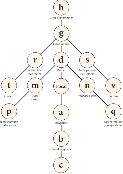
Figure 1: The kinship network. The network of kin defined in Goodman, Keyfitz, and Pullum (1974) and Keyfitz and Caswell (2005). The symbols (a,b, etc.) are used here to denote the age distribution vectors of each type of kin of Focal. That is, e.g.,a(x)is the expected age distribution of daughters at agexof Focal.
Focal
h
g
r
d
s
t
m
n
v
p
a
q
b
c
Great-grandmotherGrandmother
Mother
Daughters
Granddaughters
Great-granddaughters Aunts older
than mother Aunts youngerthan mother
Nieces through younger sisters Nieces through
older sisters
Older
sisters Younger sisters Cousins
Cousins
Figure 1, modified from Goodman, Keyfitz, and Pullum (1974), shows a portion of this network. I consider only direct matrilineal descent (mothers, daughters, granddaughters, etc.) and only consanguineal relationships. Each of these 14 types of kin is described by a population vector (a(x),b(x), . . . ), as indicated in Figure 1. Keeping track of 14 types of kin poses notational challenges, because some symbols need to be used for other purposes. The rationale behind the exclusion of some letters from the assignments in Figure 1 is as follows. The symbolejis already in use as thejth unit vector (i.e., a vector
with a 1 in thejth entry and zeros elsewhere),Fis the fertility matrix,iandjare reserved for indices and counters,kis used to refer to a generic kin,`is the survivorship function,
ois generally confusing as a symbol,Uis the transition and survival matrix,wthe stable age distribution, andxis age.
The network in Figure 1 can be extended further in the direction of descendants, ancestors, and chains derived from the siblings of ancestors (as, for example, cousins are the descendants of the siblings of the mother of Focal). I will discuss some of these descendants below.
Armed with these definitions and the general model in (4) and (5), we can proceed to derive models for the dynamics of each type of kin.
2.1.1 Daughters and descendants
Each type of descendent depends on the reproduction of another type of descendent, or of Focal herself.
a(x)= daughters of Focal. Daughters are the result of the reproduction of Focal. Since Focal is assumed to be alive at agex, the subsidy vector isβ(x) =Fex, whereex
is the unit vector for agex. Because we may be sure that Focal has no daughters when she is born, the initial condition isa0=0. Thus
a(x+ 1) = Ua(x) +Fex (6)
a0 = 0. (7)
b(x)= granddaughters of Focal. Granddaughters are the children of the daughters of Focal. At agexof Focal, these daughters have age distributiona(x), soβ(x) =
Fa(x). Because Focal has no granddaughters at birth, the initial condition is0;
b(x+ 1) = Ub(x) +Fa(x) (8)
b0 = 0. (9)
of reproduction by the granddaughters of Focal, with an initial condition of0.
c(x+ 1) = Uc(x) +Fb(x) (10)
c0 = 0. (11)
The extension to arbitrary levels of direct descendants is obvious. Letkn, in this
case, be the age distribution of descendants of leveln, wheren= 1denotes chil-dren. Then
kn+1(x+ 1) =Ukn+1(x) +Fkn(x) (12)
with the initial condition
kn+1(0) =kn(0) = 0
2.1.2 Mothers and ancestors
The surviving mothers and other direct ancestors depend on the age of those ancestors at the time of the birth of Focal.
d(x)= mothers of Focal. The population of mothers of focal consists of at most a single individual (step-mothers are not considered here). It has an expected age distribu-tion, and is subject to survival according toU. No new mothers arrive after Focal’s birth, so the subsidy term isβ(x) =0.
At the time of Focal’s birth, she has exactly one mother, but we do not know her age. Hence the initial age distributiond0of mothers is a mixture of unit vectorsei; the mixing distribution is the distributionπof ages of mothers given by (3). Thus,
d(x+ 1) = Ud(x) +0 (13)
d0 =
X
i
πiei = π. (14)
g(x)= grandmothers of Focal. The grandmothers of Focal are the mothers of the mother of Focal. No new grandmothers appear, so once again the subsidy termβ(x) =0. The age distribution of grandmothers at the birth of Focal is the age distribution of the mothers of Focal’s mother, at the age of Focal’s mother when Focal is born. The age of Focal’s mother at Focal’s birth is unknown, so the initial age distribution of grandmothers is a mixture of the age distributionsd(x)of mothers, with mixing distributionπ:
g(x+ 1) = Ug(x) +0 (15)
g0 =
X
i
h(x)= great-grandmothers of Focal. Again, the subsidy term isβ(x) =0. The initial condition is a mixture of the age distributions of the grandmothers of Focal, with mixing distributionπ:
h(x+ 1) = Uh(x) +0 (17)
h0 =
X
i
πig(i). (18)
The extension to arbitrary levels of direct ancestry is clear. Letknbe, in this case, the age distribution of ancestors of leveln, wheren = 1denotes mothers. Then the dynamics and initial conditions are
kn+1(x+ 1) = Ukn+1(x) +0 (19)
kn+1(0) = X
i
πikn(i). (20)
Note that, because Focal has at most one mother, grandmother, etc., the expected number of mothers, grandmothers, etc. is also the probability of having a living mother, grandmother, etc.
2.1.3 Sisters and nieces
The sisters of Focal, and their children, who are the nieces of Focal, form the first set of side branches in the kinship network of Figure 1. Following Goodman, Keyfitz, and Pul-lum (1974), it is convenient to divide the sisters of Focal into older and younger sisters, because they follow different dynamics.
m(x)= older sisters of Focal. Once Focal is born, she accumulates no more older sis-ters, so the subsidy term isβ(x) = 0. At Focal’s birth, her older sisters are the childrena(i)of the mother of Focal at the ageiof Focal’s mother at Focal’s birth. This age is unknown, so the initial conditionm0is a mixture of the age distribu-tions of children with mixing distributionπ.
m(x+ 1) = Um(x) +0 (21)
m0 = X
i
πia(i). (22)
n(x)= younger sisters of Focal. Focal has no younger sisters when she is born, so the initial condition isn0=0. Younger sisters are produced by reproduction of Focal’s
mother, so the subsidy term is the reproduction of the mothers at agexof Focal.
n(x+ 1) = Un(x) +Fd(x) (23)
p(x)= nieces through older sisters of Focal. At the birth of Focal, these nieces are the granddaughters of the mother of Focal, so the initial condition is mixture of grand-daughters with mixing distribution π. New nieces through older sisters are the result of reproduction by the older sisters, at agex, of Focal.
p(x+ 1) = Up(x) +Fm(x) (25)
p0 =
X
i
πib(i). (26)
q(x)= nieces through younger sisters of Focal. At the birth of Focal she has no younger sisters, and hence has no nieces through these sisters. Thus the initial condition is
q0=0. New nieces are produced by reproduction of the younger sisters of Focal.
q(x+ 1) = Uq(x) +Fn(x) (27)
q0 = 0. (28)
2.1.4 Aunts and cousins
Aunts and cousins form another level of side branching on the kinship network; their dy-namics follow the same principles as those for sisters and nieces.
r(x)= aunts older than mother of Focal. These are the older sisters of the mother of Focal. Once Focal is born, her mother accumulates no new older sisters, so the subsidy term isβ(x) =0. The initial age distribution of these aunts, at the birth of Focal, is a mixture of the age distributionsmof older sisters, with mixing distribu-tionπ
r(x+ 1) = Ur(x) +0 (29)
r0 =
X
i
πim(i). (30)
s(x)= aunts younger than mother of Focal. These are the younger sisters of the mother of Focal. These aunts are the children of the grandmother of Focal, and thus the subsidy term comes from reproduction by the grandmothers of Focal. The initial age distribution of these aunts, at the birth of Focal, is a mixture of the age distri-butionsnof younger sisters, with mixing distributionπ.
s(x+ 1) = Us(x) +Fg(x) (31)
s0 =
X
i
t(x)= cousins from aunts older than mother of Focal. These are the children of the older sisters of the mother of Focal, and thus the nieces of the mother of Focal through her older sisters. The subsidy term comes from reproduction by the older sisters of the mother of Focal.The initial condition is a mixture of the age distribu-tions of nieces through older sisters, with mixing distributionπ.
t(x+ 1) = Ut(x) +Fr(x) (33)
t0 = X
i
πip(i). (34)
v(x)= cousins from aunts younger than mother of Focal. These are the nieces of the mother of Focal through her younger sisters. The subsidy term comes from re-production by the younger sisters of the mother of Focal. The initial condition is a mixture of the age distributions of nieces through younger sisters, with mixing distributionπ.
v(x+ 1) = Uv(x) +Fs(x) (35)
v0 =
X
i
πiq(i). (36)
2.1.5 Model summary
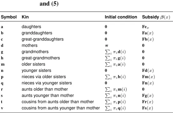
Table 1: Summary of the components of the kin model given in equations (4) and (5)
Symbol Kin Initial condition Subsidyβ(x)
a daughters 0 Fex
b granddaughters 0 Fa(x)
c great-granddaughters 0 Fb(x)
d mothers π 0
g grandmothers P
iπid(i) 0
h great-grandmothers P
iπig(i) 0
m older sisters P
iπia(i) 0
n younger sisters 0 Fd(x)
p nieces via older sisters P
iπib(i) Fm(x)
q nieces via younger sisters 0 Fn(x)
r aunts older than mother P
iπim(i) 0
s aunts younger than mother P
iπin(i) Fg(x)
t cousins from aunts older than mother P
iπip(i) Fr(x)
v cousins from aunts younger than mother P
iπiq(i) Fs(x)
3. Derived properties of kin
Because the model provides the age distributions of all types of kin, it makes it possible to compute what might be called derived properties of the age distribution of kin. These might be linear functions of the age distribution, leading to a model
k(x+ 1) = Uk(x) +β(x) (37)
k(0) = k0 (38)
y(x) = Ψ(x)k(x) (39)
wherey(x)is a vector of the property in question at agexof focal, andΨ(x)is the ma-trix of a linear transformation from the age distribution to the property vector. Examples of such derived properties include
1. Numbers of kin, in which caseΨ(x) =1T
ω.
2. Prevalence, in which caseΨ(x)is a vector containing, e.g., age-specific prevalence of some condition, such as disease, disability, health, labor force participation, etc.
Ψ=
1 1 0 0 0 0
0 0 1 1 0 0
0 0 0 0 1 1
(40)
4. Coresidence probability. This is actually a special case of prevalence, where the condition is “coresiding with Focal.”
Nonlinear functions ofk(x)(e.g., dependency ratios) can also be calculated. One im-portant set of such derived properties are the mean, and other moments, of the age of a particular set of relatives.
5. Moments of age distribution. Define vectors
ci= 0.5i 1.5i · · · (ω−0.5)i T
i= 1, 2,. . .. (41)
Defineµi as theith moment of age (so that the mean age isµ1). Theith moment
of the age of the kink(x)is
µi(x) =cTi k(x)
kk(x)k (42)
(provided, of course, thatkk(x)k>0). In particular, the mean and variance of the age of kin are
E(µ(x)) = µ1(x) (43)
V(µ(x)) = µ2(x)−µ1(x)2. (44)
A useful operation is the aggregation of kin types. It is possible to aggregate the kinship network in Figure 1 by adding the appropriate vectors.
6. Aggregation of kin.
Figure 1 disaggregates the older and younger sisters of Focal. The total number of sisters is the sum of the older and younger sisters,
sisters=m(x) +n(x). (45)
An important aggregation is that based on degree. Degrees of kinship are defined in both civil and religious law, and determine ability to marry, aspects of inheritance, jury selection, restrictions on nepotism in hiring, and other fascinating things. Ac-cording to one version,
first degree kin = a(x) +d(x) (46)
second degree kin = b(x) +g(x) +m(x) +n(x) (47)
4. Death of kin
The experience of the death of close relatives can have long-lasting effects on an indi-vidual (e.g., Umberson et al. 2017). The experience by Focal of the death of kin can be calculated directly from the kinship model. To do so, we expand the kin population vector
kto include dead as well as living kin, creating a new vector
˜
k=
kliving kdead
. (49)
The tilde distinguishes this multistate vector from the vector containing only living relatives.
Two possibilities present themselves for calculations with deceased relatives. We can calculate the deaths of kin experienced by Focal at a given agex, or the cumulative deaths experienced by Focal up to a given agex. The calculations require only a simple change to the matricesUandF, and the vectork0, in order to account for both living
and dead kin.
In order forkdead(x)to capture the age distribution of the deaths experienced by Focal at agex,Uis replaced by the block-structured matrix
˜
U=
U 0
M 0
. (50)
The mortality matrixMcontains the transition probabilities from ages of kin (columns ofM) to the state of being dead at a particular age (rows ofM). Thus
M=D(q). (51)
The matrix0in the lower right corner ofU˜ removes the dead individuals after a single time step. The result is the projection
˜
k(x+ 1) = ˜Uk˜(x) + ˜β(x). (52)
The fertility matrixFthat appears inβ(x)is replaced by the matrix
˜
F=
F 0
0 0
(53)
To calculate the cumulative deaths experienced by Focal up to agex, rather than the deaths experienced at a given age, the matrixUis replaced by
˜
U=
U 0
M I
(54)
where again
M=D(q).
The identity matrix in the lower right corner ofU˜ keeps the dead kin in an absorbing state corresponding to their age at death.
The initial condition˜k0for the partitioned kin vector accounts for the fact that Focal
has experienced no deaths at the time of her birth. Thus,
˜
k0=
k
0 0
(55)
wherek0is the initial vector for kinkas described in Table 1.
These calculations can be extended to include deaths that occur before the birth of Focal (e.g., “your grandmother died before you were born”) or after the death of Focal (e.g., Queen Victoria died in 1901 at the age of 81, but of her 87 great-grandchildren, several were born after 1901, and of course other descendants continue to appear). These extensions will be presented elsewhere.
5. An example: Changes in the kinship network of Japan
As an example of the model, I explore the implications for the kinship network of changes in the mortality and fertility schedules of Japanese women from 1947 and 2014. This period saw dramatic changes in both mortality (life expectancy increased by about 60%) and fertility (total fertility rate decreased by 70% and the net reproductive rate declined by about 60%), as shown in Figure 2.
1947 2014 % change life exp 54 87 +61%
TFR 4.6 1.4 −70%
R0 1.7 0.7 −59%
The matricesUandFare created from the mortality (qx) schedules and the age-specific
Note that this is just an example; it is not intended as a detailed examination of the kinship demography of Japan. Also note that for convenience I will speak of, e.g., “Japan in 1947” instead of the more correct “a stable population subject to the period mortality and fertility schedules of Japan as measured in 1947.”
For the convenience of the reader, results of the calculations are collected together, in graphical form, for selected types of kin, in Section 7. For the truly curious, an Online Supplementary collection contains figures for all types of kin for each of the categories examined here.
Figure 2: Mortality and fertility. The mortality and fertility schedules for Japanese women in 1947 and 2014
a) Mortality
0 20 40 60 80 100 120
Age 10-5
10-4 10-3 10-2 10-1 100
Mortality qx
1947 2014
a) Fertility
0 20 40 60 80 100 120
Age 0
0.05 0.1 0.15 0.2 0.25 0.3
Fertility
1947 2014
Source: Data from Human Mortality Database (2018) and Human Fertility Database (2018).
5.1 Age distributions
Figure 4 shows the age distributions of mothers, grandmothers, daughters, granddaugh-ters, sisgranddaugh-ters, and cousins, for a Focal individual aged 30 and aged 70. The mothers of Focal at 30 are slightly older under 2014 rates than under 1947 rates, and far more com-mon. Focal at age 70 has essentially no chance of a living mother in 1947, but still some chance of a very elderly living mother in 2014 (Figure 4a). The situation with grand-mothers is similar (Figure 4b), but more extreme. No living grandgrand-mothers remain at age 70 of Focal, but at age 30 grandmothers are about 4 times more likely and about 10 years older in 2014 compared to 1947.
The age distributions of sisters and cousins (Figure 4e and f) show the effects of the mortality difference between 1947 and 2014. In 1947, Focal loses about 40% of her sisters and cousins between the ages of 30 and 70. In 2014, there is almost no loss of sisters or cousins between these ages.
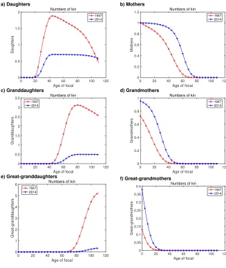
5.2 Numbers of kin
Figure 5 shows the numbers of living kin as a function of the age of Focal. Comparing daughters, granddaughters, and great-granddaughters (Figures 5a, c, and e) shows the in-tegrated effects of mortality and fertility changes between 1947 and 2014. In 1947, Focal reaches a peak of about 3 times more daughters than does Focal in 2014, but the number of living daughters declines after about age 40 of Focal. In 2014, fewer daughters are produced, and there is hardly any decline in the number of daughters due to mortality. Comparing the numbers of granddaughters and great-granddaughters shows the pattern hinted at in Figure 4: Focal in 1947 has progressively more descendants in each genera-tion, while Focal in 2014 has fewer.
For ancestors (Figures 5b, d, and f), the intergenerational pattern is reversed. Focal in 2014 is more likely to have a surviving mother than Focal in 1947; the differential increases for grandmothers and great-grandmothers.
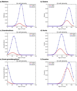
5.3 Prevalence of dementia
Figure 3: Dementia prevalence. Age-specific prevalence of dementia among Japanese women in 2015
0 20 40 60 80 100 120
Age
0 0.1 0.2 0.3 0.4 0.5 0.6
Prevalence of dementia 2015
Source: Data from Fukawa (2018).
Figure 6 shows the numbers of kin with dementia, as a function of the age of Focal, in 1947 and 2014. Focal is far more likely to have a mother, grandmother, or great-grandmother with dementia in 2014 than in 1947 (Figures 6a, c, and d). The difference is large (about 7-fold for mothers, even greater for grandmothers and great-grandmothers). The same holds for sisters (Figure 6b) and aunts (Figure 4d). Among cousins, the differ-ence is not as great, but the prevaldiffer-ence of dementia among kin is still higher in 2014 than 1947.
5.4 Mean and variance of ages of kin
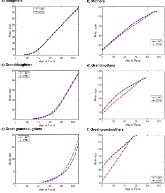
The means and standard deviations of the ages of several types of kin are shown in Fig-ures 7 and 8. Mean ages naturally increase with the age of Focal. For both ancestors (mothers, grandmothers, etc.) and descendants (daughters, granddaughters, etc.) there is little difference between 1947 and 2014, perhaps because the timing of fertility does not change much between those years.
Focal, with no consistent differences between 1947 and 2014 rates. Maximum standard deviations are on the order of 6 to 8 years. Differences between 1947 and 2014 rates are small relative to other properties, because the timing of reproduction shows only minor changes.
5.5 Dependency of kin
Figure 9 shows, as a function of the age of Focal, the numbers of kin in three categories of dependence. Young dependence is defined here as ages 0–15, old dependence as ages greater than 65, and independence as ages 16–65. These could easily be replaced with more detailed descriptors of economic contribution.
Figure 9 shows results for 1947 in solid lines, and 2014 in dashed lines. Depen-dent children, grandchildren, and great-grandchildren accumulate earlier, and much more rapidly, for Focal in 1947 than in 2014. Focal in 1947 was much more likely to have de-pendent great-granddaughters than in 2014, reflecting the greater numbers of descendants under those conditions (cf. Figure 5).
The pattern is reversed when considering dependent mothers, grandmothers, and great-grandmothers, which are much more abundant in 2014 than in 1947. A short de-scription of the pattern would be that Focal in 1947 confronts more dependent children and descendants, but in 2014 she is faced with more dependent parents and ancestors.
5.6 Death of kin
Turning now to the death of kin, Figure 10 shows the experience of death of kin at each age of Focal, and Figure 11 shows the cumulative deaths experienced up to each age of Focal. As far as deaths of kin are concerned, the world changed dramatically between 1947 and 2014. The deaths of daughters, granddaughters, mothers, sisters, and aunts occur earlier and far more frequently under the rates of 1947. Focal in 2014 will almost never experience the death of a daughter or granddaughter (Figures 10a, b; 11a and b). It is rare for Focal in 2014 to experience the death of a sister before the age of 60, but in 1947 such deaths occur frequently from the birth of Focal.
6. Discussion
coupled system of non-autonomous matrix difference equations) may sound more com-plicated. It is not. As with any dynamical system, the dynamic equations carry out the necessary integrations, but with much more flexibility. Together, the assumptions of ho-mogeneity and time invariance make it possible to extend the equations for parents and children to include all the kin shown in Table 1, and even beyond that, as in equation (12) for arbitrary levels of descendants. A brief comparison of the results given by Good-man, Keyfitz, and Pullum (1974) and those produced by this model shows qualitative agreement, but with quantitative differences probably due to the (unspecified) choice of numerical integration methods applied to the coarsely-resolved (5 year age intervals) life tables available in 1974. The freedom from the need to carry out such numerical integra-tion, and from the error propagation involved with multiple integrals, is a strength of the present method.
One advantage of formal mathematical specification is that it makes explicit the assumptions underlying an analysis. As Goodman, Keyfitz, and Pullum (1974) pointed out repeatedly, these results are not expected to give the same results as a census of the kin of individuals of different ages, precisely because the assumptions are counterfactuals. The value of comparing calculated kinship structures with empirical kinship censuses is not to test the mathematics, but to see how the actual kinship network is warped by violation of the assumptions.
It will be interesting to relax the assumptions. Relaxing the assumption of homo-geneity will require extending the state space to include additional dimensions affect-ing kinship (marital status is one obvious possibility) in age×stage or multistate models (Caswell et al. 2018). Parity dependence is another important dimension. Schoen (2019) presents theory for close kin in terms of parity progression, under the assumption that all women live to the end of their reproductive years and that mortality does not affect children. He emphasizes that parity progression, when used as a model for fertility, auto-matically captures some important aspects of sibship and family formation. Incorporating age and parity into the reproductive component of the model here will permit exploration of these effects under less restrictive assumptions.
The analysis here, and the example in Section 5, are formulated in terms of female survival and fertility, and relatives through the female line. It is clearly possible to carry out the same analysis using male survival and fertility; it will be interesting to do so to see the effect of the extended timing of male fertility, especially in hunter–gatherer pop-ulations (e.g., Tuljapurkar, Puleston, and Gurven 2007). A generalization to include both male and female kin, through both male and female lines of descent, will be presented elsewhere.
assumption of time invariance will require the extension of the time domain to include not only the agexof Focal but also the time before or after the birth of Focal.
Finally, note that the results of these calculations, like those of Goodman, Keyfitz, and Pullum (1974), provideexpectedage distributions. While the kin of Focal form a pop-ulation, that population is small and thus subject to demographic stochasticity. Stochastic versions of the model could be constructed using branching process methods, as dis-cussed by Pullum (1982). Connections of multitype branching processes to matrix popu-lation models are explored by Pollard (1966), Caswell (2001), and Caswell and Vindenes (2018). Alternatively, stochastic realizations of the dynamic models here, or even com-plete microsimulation models (e.g., Wachter 1997), can provide information on variances and higher moments.
7. Figures
Figure 4: Age distributions. The age distributions of several types of kin, at ages 30 (solid lines) and 70 (dashed lines) of Focal. Calculated from the vital rates of Japan in 1947 (red) and 2014 (blue).
a) Mothers
0 20 40 60 80 100
Age of kin 0 0.01 0.02 0.03 0.04 0.05 0.06 0.07 0.08 Mothers Age distribution 30 1947 30 2014 70 1947 70 2014 b) Grandmothers
0 20 40 60 80 100
Age of kin
0 0.005 0.01 0.015 0.02 0.025 0.03 Grandmothers Age distribution 30 1947 30 2014 70 1947 70 2014 c) Daughters
0 20 40 60 80 100
Age of kin 0 0.02 0.04 0.06 0.08 0.1 0.12 0.14 Daughters Age distribution 30 1947 30 2014 70 1947 70 2014 d) Granddaughters
0 20 40 60 80 100
Age of kin
0 0.05 0.1 0.15 Granddaughters Age distribution 30 1947 30 2014 70 1947 70 2014 e) Sisters
0 20 40 60 80 100
Age of kin 0 0.02 0.04 0.06 0.08 0.1 Sisters Age distribution 30 1947 30 2014 70 1947 70 2014 f) Cousins
0 20 40 60 80 100
Age of kin
Figure 5: Numbers. Numbers of kin of several types, as a function of the age of Focal. Calculated from the vital rates of Japan in 1947 (red) and 2014 (blue).
a) Daughters
0 20 40 60 80 100 120
Age of focal 0 0.5 1 1.5 2 Daughters
Numbers of kin
1947 2014
b) Mothers
0 20 40 60 80 100 120
Age of focal 0 0.2 0.4 0.6 0.8 1 1.2 Mothers
Numbers of kin
1947 2014
c) Granddaughters
0 20 40 60 80 100 120
Age of focal 0 0.5 1 1.5 2 2.5 3 3.5 Granddaughters
Numbers of kin
1947 2014
d) Grandmothers
0 20 40 60 80 100 120
Age of focal 0 0.2 0.4 0.6 0.8 1 Grandmothers
Numbers of kin
1947 2014
e) Great-granddaughters
0 20 40 60 80 100 120
Age of focal 0 1 2 3 4 5 6 Great-granddaughters
Numbers of kin
1947 2014
f) Great-grandmothers
0 20 40 60 80 100 120
Age of focal 0 0.05 0.1 0.15 0.2 0.25 0.3 0.35 0.4 Great-grandmothers
Numbers of kin
Figure 6: Kin with dementia. Numbers of kin of several types suffering from dementia, as a function of the age of Focal. Calculated from the vital rates of Japan in 1947 (red) and 2014 (blue), using dementia prevalence rates for Japanese females in 2015.
a) Mothers
0 20 40 60 80 100 120
Age of Focal 0 0.02 0.04 0.06 0.08 0.1 0.12 0.14 Mothers
Kin with dementia
1947 2014
b) Sisters
0 20 40 60 80 100 120
Age of Focal 0 0.02 0.04 0.06 0.08 0.1 Sisters
Kin with dementia
1947 2014
c) Grandmothers
0 20 40 60 80 100 120
Age of Focal 0 0.02 0.04 0.06 0.08 0.1 0.12 0.14 Grandmothers
Kin with dementia
1947 2014
d) Aunts
0 20 40 60 80 100 120
Age of Focal
0 0.01 0.02 0.03 0.04 0.05 0.06 0.07 0.08 Aunts
Kin with dementia
1947 2014
e) Great-granddaughters
0 20 40 60 80 100 120
Age of Focal 0 0.02 0.04 0.06 0.08 0.1 0.12 Great-grandmothers
Kin with dementia
1947 2014
f) Cousins
0 20 40 60 80 100 120
Age of Focal 0 0.01 0.02 0.03 0.04 0.05 Cousins
Kin with dementia
Figure 7: Mean age. The mean age of kin of several types, as a function of the age of Focal. Calculated from the vital rates of Japan in 1947 (red) and 2014 (blue). The mean age is set to zero when the number of kin drops below10−9.
a) Daughters
0 20 40 60 80 100
Age of Focal 0 10 20 30 40 50 60 70 80 Mean age 1947 2014 b) Mothers
0 20 40 60 80 100
Age of Focal 20 40 60 80 100 120 Mean age 1947 2014 c) Granddaughters
0 20 40 60 80 100
Age of Focal 0 10 20 30 40 50 Mean age 1947 2014 d) Grandmothers
0 20 40 60 80 100
Age of Focal 50 60 70 80 90 100 110 120
Mean age 19472014
e) Great-granddaughters
0 20 40 60 80 100
Age of Focal 0 5 10 15 20 Mean age 1947 2014 f) Great-grandmothers
0 20 40 60 80 100
Figure 8: Standard deviation of age. The standard deviation (in years) of the age of kin of several types, as a function of the age of Focal. Calculated from the vital rates of Japan in 1947 (red) and 2014 (blue).
a) Daughters
0 20 40 60 80 100
Age of Focal 0 1 2 3 4 5 6 7
SD of age
1947 2014
b) Mothers
0 20 40 60 80 100
Age of Focal 0 1 2 3 4 5 6
SD of age
1947 2014
c) Granddaughters
0 20 40 60 80 100
Age of Focal 0 2 4 6 8 10
SD of age
1947 2014
d) Grandmothers
0 20 40 60 80 100
Age of Focal 0 1 2 3 4 5 6 7 8
SD of age
1947 2014
e) Great-granddaughters
0 20 40 60 80 100
Age of Focal 0 2 4 6 8 10
SD of age
1947 2014
f) Great-grandmothers
0 20 40 60 80 100
Age of Focal 0 1 2 3 4 5 6 7
SD of age
Figure 9: Dependency of kin. Numbers of kin, of several types, in three different dependency categories: young dependents aged 0–16, old dependents aged more than 65, and independent kin aged 16–65, as a function of the age of Focal. Calculated from the vital rates of Japan in 1947 (solid lines) and 2014 (dashed lines).
a) Daughters
0 20 40 60 80 100
Age of Focal 0 0.5 1 1.5 2 Daughters Dependency young dep indep old dep b) Granddaughters
0 20 40 60 80 100
Age of Focal 0 0.5 1 1.5 2 2.5 3 Granddaughters Dependency young dep indep old dep c) Great-granddaughters
0 20 40 60 80 100
Age of Focal 0 0.5 1 1.5 2 2.5 3 3.5 Great-granddaughters Dependency young dep indep old dep d) Mothers
0 20 40 60 80 100
Age of Focal 0 0.2 0.4 0.6 0.8 1 Mothers Dependency young dep indep old dep e) Grandmothers
0 20 40 60 80 100
Age of Focal 0 0.1 0.2 0.3 0.4 0.5 0.6 0.7 0.8 Grandmothers Dependency young dep indep old dep f) Great-grandmothers
0 20 40 60 80 100
Figure 10: Experienced deaths. Numbers of deaths of kin, of several types, experienced by Focal at each age. Calculated from the vital rates of Japan in 1947 and 2014.
a) Daughters
0 20 40 60 80 100 120
Age of Focal 0 0.01 0.02 0.03 0.04 0.05 Daughters Experienced deaths 1947 2014 b) Granddaughters
0 20 40 60 80 100 120
Age of Focal 0 0.005 0.01 0.015 0.02 0.025 0.03 Granddaughters Experienced deaths 1947 2014 c) Mothers
0 20 40 60 80 100 120
Age of Focal 0 0.005 0.01 0.015 0.02 0.025 0.03 0.035 0.04 Mothers Experienced deaths 1947 2014 d) Grandmothers
0 20 40 60 80 100 120
Age of Focal 0 0.005 0.01 0.015 0.02 0.025 0.03 0.035 Grandmothers Experienced deaths 1947 2014 e) Sisters
0 20 40 60 80 100 120
Age of Focal 0 0.01 0.02 0.03 0.04 0.05 Sisters Experienced deaths 1947 2014 f) Aunts
0 20 40 60 80 100 120
Figure 11: Cumulative deaths. The cumulative numbers of deaths of kin experienced by Focal up to each age. Calculated from the vital rates of Japan in 1947 and 2014.
a) Daughters
0 20 40 60 80 100 120
Age of Focal 0 0.5 1 1.5 2 Daughters Cumulative deaths 1947 2014 b) Granddaughters
0 20 40 60 80 100 120
Age of Focal 0 0.2 0.4 0.6 0.8 1 1.2 1.4 Granddaughters Cumulative deaths 1947 2014 c) Mothers
0 20 40 60 80 100 120
Age of Focal 0 0.2 0.4 0.6 0.8 1 1.2 Mothers Cumulative deaths 1947 2014 d) Grandmothers
0 20 40 60 80 100 120
Age of Focal 0 0.2 0.4 0.6 0.8 1 Grandmothers Cumulative deaths 1947 2014 e) Sisters
0 20 40 60 80 100 120
Age of Focal
0 0.5 1 1.5 2 2.5 Sisters Cumulative deaths 1947 2014 f) Aunts
0 20 40 60 80 100 120 Age of Focal
8. Acknowledgments
References
Bartholomew, D.J. (1982).Stochastic models for social processes. New York: Wiley.
Bengtson, V.L. (2001). Beyond the nuclear family: The increasing importance of multi-generational bonds.Journal of Marriage and Family63(1): 1–16. doi:10.1111/j.1741-3737.2001.00001.x.
Brennan, E.R., James, A.V., and Morrill, W.T. (1982). Inheritance, demographic struc-ture, and marriage: A cross-cultural perspective.Journal of Family History7(3): 289– 298. doi:10.1177/036319908200700304.
Burch, T.K. (1995). Estimating the Goodman, Keyfitz, Pullum kinship equations: An alternative procedure. Mathematical Population Studies5(2): 161–170. doi:10.1177/ 036319908200700304.
Caswell, H. (2001). Matrix population models: Construction, analysis, and interpreta-tion. Sunderland: Sinauer, 2nded.
Caswell, H. (2008). Perturbation analysis of nonlinear matrix population models. Demo-graphic Research18(3): 59–116.doi:10.4054/DemRes.2008.18.3.
Caswell, H., de Vries, C., Hartemink, N., Roth, G., and van Daalen, S.F. (2018). Age stage-classified demographic analysis: A comprehensive approach. Ecological Mono-graphs88(4): 560–584. doi:10.1002/ecm.1306.
Caswell, H. and Vindenes, Y. (2018). Demographic variance in heterogeneous populations: Matrix models and sensitivity analysis. Oikos 127(5): 648–663.
doi:10.1111/oik.04708.
Coale, A.J. (1972). The growth and structure of human populations: A mathematical approach. Princeton: Princeton University Press.
Croft, D.P., Johnstone, R.A., Ellis, S., Nattrass, S., Franks, D., Brent, L.J., Mazzi, S., Balcomb, K.C., Ford, J.K., and Cant, M.A. (2017). Reproductive conflict and the evolution of menopause in killer whales. Current Biology 27(2): 298–304.
doi:10.1016/j.cub.2016.12.015.
DeRigne, L. and Ferrante, S. (2012). The sandwich generation: A review of the literature. Florida Public Health Review9: 95–104.
Dykstra, P.A. (2010). Intergenerational family relationships in ageing societies. New York: United Nations. https://www.unece.org/fileadmin/DAM/pau/ docs/age/2010/ Intergenerational-Relationships/ECE-WG.1-11.pdf.
Fukawa, T. (2018). Prevalence of dementia among the elderly population of japan.Health and Primary Care2(4): 1–6.doi:10.15761/HPC.1000147.
Gisser, R. and Ediev, D.M. (2019). Having ancestors alive: Trends and prospects in ageing Europe. In: Schoen, R. (ed.).Analytical family demography. Cham: Springer: 241–274.doi:10.1007/978-3-319-93227-9 11.
Goldman, N. (1978). Estimating the intrinsic rate of increase of population from the average numbers of younger and older sisters. Demography 15(4): 499–507.
doi:10.2307/2061202.
Goodman, L.A., Keyfitz, N., and Pullum, T.W. (1974). Family formation and the fre-quency of various kinship relationships. Theoretical Population Biology5(1): 1–27.
doi:10.1016/0040-5809(74)90049-5.
Greenwood, M. and Yule, G.U. (1914). On the determination of size of family and of the distribution of characters in order of birth from samples taken through mem-bers of the sibships. Journal of the Royal Statistical Society 77(2): 179–199.
doi:10.2307/2339801.
Harpending, H. and Draper, P. (1990). Estimating parity of parents: Application to the history of infertility among the !Kung of Southern Africa.Human Biology62(2): 195– 203.
Himes, C.L. (1992). Future caregivers: Projected family structures of older persons. Journal of Gerontology47(1): S17–S26.doi:10.1093/geronj/47.1.S17.
Hrdy, S.B. (2009). Mothers and others. Cambridge: Harvard University Press.
Human Fertility Database (2018). Human fertility database [electronic resource]. Rostock and Vienna: Max Planck Institute for Demographic Research and the Vienna Institute of Demography.http://www.humanfertility.org.
Human Mortality Database (2018). Human mortality database [electronic resource]. Berkeley and Rostock: University of California, Berkeley and Max Planck Institute for Demographic Research.http://www.mortality.org.
Jones, J.H. and Morris, M. (2003). Orphans and ‘grandorphans’ in sub-Saharan Africa: The consequences of dependent mortality. Paper presented at the Annual Meeting of the Population Association of America, Minneapolis, USA, May 1–3, 2003.
Kazeem, A. and Jensen, L. (2017). Orphan status, school attendance, and relationship to household head in Nigeria. Demographic Research36(22): 659–690. doi:10.4054/ DemRes.2017.36.22.
Krishnamoorthy, S. (1979). Family formation and the life cycle. Demography16(1): 121–129.doi:10.2307/2061083.
Lahdenper¨a, M., Gillespie, D.O., Lummaa, V., and Russell, A.F. (2012). Severe inter-generational reproductive conflict and the evolution of menopause. Ecology Letters 15(11): 1283–1290.doi:10.1111/j.1461-0248.2012.01851.x.
Leslie, P.H. (1945). On the use of matrices in certain population mathematics.Biometrika 33(3): 183–212. doi:10.1093/biomet/33.3.183.
Lotka, A.J. (1931). Orphanhood in relation to demographic factors.Metron9: 37–109.
Mare, R.D. and Song, X. (2015). The changing demography of multigenerational re-lationships. Paper presented at the Annual Meeting of the Population Association of America, San Diego, USA, April 30–May 2, 2015.
McDaniel, C. and Hammel, E. (1984). A kin-based measure of r and an evaluation of its effectiveness.Demography21(1): 41–51.doi:10.2307/2061026.
Pascual, M. and Caswell, H. (1991). The dynamics of a size-classified benthic pop-ulation with reproductive subsidy. Theoretical Population Biology39(2): 129–147.
doi:10.1016/0040-5809(91)90032-B.
Pollard, J.H. (1966). On the use of the direct matrix product in analysing certain stochastic population models.Biometrika53(3–4): 397–415. doi:10.1093/biomet/53.3-4.397.
Pollard, J.H. (1968). A note on the age structures of learned societies. Journal of the Royal Statistical Society Series A: General131(4): 569–578.doi:10.2307/2343724.
Pullum, T.W. (1982). The eventual frequencies of kin in a stable population.Demography 19(4): 549–565. doi:10.2307/2061018.
Pullum, T.W. and Wolf, D.A. (1991). Correlations between frequencies of kin. Demog-raphy28(3): 391–409. doi:10.2307/2061018.
Roche, S. (2010). From youth bulge to conflict: The case of Tajikistan. Central Asian Survey29(4): 405–419. doi:10.1080/02634937.2010.533968.
Roche, S. (2014). Domesticating youth: Youth bulges and their socio-political implica-tions in Tajikistan. New York: Berghahn Books.
Schoen, R. (2019). Parity progression and the kinship network. In: Schoen, R. (ed.). Analytical family demography. Cham: Springer: 189–199.
Song, X. and Campbell, C.D. (2017). Genealogical microdata and their significance for social science. Annual Review of Sociology 43: 75–99. doi:10.1146/annurev-soc-073014-112157.
Song, X. and Mare, R.D. (2017). Short-term and long-term educational mobility of fam-ilies: A two-sex approach. Demography54(1): 145–173. doi:10.1007/s13524-016-0540-4.
Stecklov, G. (2002). The economic boundaries of kinship in Cˆote d’Ivoire. Population Research and Policy Review21(4): 351–375.doi:10.1023/A:1020072023054.
Tanskanen, A.O. and Danielsbacka, M. (2019). Intergenerational family relations: An evolutionary social science approach. New York: Routledge.
Tu, E.J.C., Freedman, V.A., and Wolf, D.A. (1993). Kinship and family support in tai-wan: A microsimulation approach. Research on Aging15(4): 465–486. doi:10.1177/ 0164027593154006.
Tuljapurkar, S.D., Puleston, C.O., and Gurven, M.D. (2007). Why men matter: Mating patterns drive evolution of human lifespan.PLOS One2(8): e785.doi:10.1371/journal. pone.0000785.
Umberson, D., Olson, J., Crosnoe, R., Liu, H., Pudrovska, T., and Donnelly, R. (2017). Death of family members as an overlooked source of racial disadvantage in the United States. Proceedings of the National Academy of Sciences114(5): 915–920.
doi:10.1073/pnas.1605599114.
Wachter, K.W. (1997). Kinship resources for the elderly. Philosophical Transactions of the Royal Society of London Series B: Biological Sciences352(1363): 1811–1817.
doi:10.1098/rstb.1997.0166.
Zagheni, E. (2010). The impact of the HIV/AIDS epidemic on orphanhood probabilities and kinship structure in Zimbabwe [PhD Thesis]. Berkeley: University of California, Berkeley.