Volume 40 - Article 53 | Pages 1537–1602

(1)

VOLUME 40, ARTICLE 53, PAGES 1537-1602

PUBLISHED 25 JUNE 2019

http://www.demographic-research.org/Volumes/Vol40/53/ DOI: 10.4054/DemRes.2019.40.53

Research Article

Gender differences in willingness to move for

interregional job offers

Martin Abraham

Sebastian Bähr

Mark Trappmann

This publication is part of the Special Collection on “Spatial Mobility, Family Dynamics and Gender Relations,” organized by Guest Editors Sergi Vidal and Johannes Huinink.

This open-access work is published under the terms of the Creative Commons Attribution 3.0 Germany (CC BY 3.0 DE), which permits use, reproduction, and distribution in any medium, provided the original author(s) and source are given credit.

(2)

1 Introduction 1537

2 Gender differences in willingness to move: Theoretical considerations

1540

3 Data and methods 1546

4 Empirical results 1551

4.1 Are there gender differences in willingness to move? 1565 4.2 Mechanisms explaining the gender differences in willingness to

move

1566

4.2.1 Quality of job offers 1566

4.2.2 Local embeddedness and costs of moving 1566 4.2.3 Collective decision-making at the household level 1567

5 Conclusion 1570

6 Acknowledgments 1572

References 1573

(3)

Gender differences in willingness to move for

interregional job offers

Martin Abraham1

Sebastian Bähr2

Mark Trappmann2

Abstract

BACKGROUND

Interregional job offers are an important mechanism of social mobility as they provide both career chances and opportunities to avoid unemployment. We know from the literature that couples have difficulties seizing these opportunities due to the unequal distribution of costs and benefits between partners. Consequently, couples generally show a lower willingness to move for a job offer for one of the partners. However, very little is known about the differences between men and women in assessing the attractiveness of a job-related household move.

OBJECTIVE

Focusing on all cohabitating couples, we address whether there are gender differences in willingness to move for a better job offer and how those differences can be explained.

METHODS

We employ a large household survey from Germany that includes a factorial survey experiment addressing willingness to move for a hypothetical job offer.

RESULTS

We find that (a) within couples, women show a lower willingness to move than men, but single women do not differ from single men; (b) variables resulting from standard theories on mobility contribute to the explanation of willingness to move; and (c) gender differences persist even after controlling for these variables.

CONCLUSIONS

Women show a lower willingness to move for a job when they are living with a partner in a household, and this cannot be sufficiently explained by standard theories of

(4)

household and family migration. Only gender norms contribute significantly to the explanation of these differences between sexes. Consequently, women are disadvantaged when considering interregional job offers.

CONTRIBUTION

Our findings reveal that interregional job offers contribute to gender inequality by hampering the career options of coupled women. A comparison with early results from the United States reveals that this seems to be a general pattern that cannot be explained by standard household migration theories.

1. Introduction

Regional mobility is an important mechanism of labor market mobility. As jobs are most likely to be generated in regions with dense populations and because jobs are scarce (especially for specialized employees), obtaining a better job often requires some kind of spatial mobility. Consequently, workers who are more mobile obtain higher wages (e.g., Yankow 2003; Ham, Li, and Reagan 2011) and exhibit a lower risk of unemployment spells (Pissarides and Wadsworth 1989; for an overview, see Bähr and Abraham 2016: 45).

However, mobility costs can be high and can hamper the matching process across regional labor markets. This is especially true for couples when one partner receives an incentive to move for a better job. Although the household will gain from a higher income, not all household members may benefit from the move individually. The loss of social contacts and the costs of adaptation to the new place are usually easier to compensate for the job mover. Moreover, if both partners are employed, couples face the ‘tied mover problem’ (Mincer 1978). Since it is unlikely that both partners will get a better job offer in the same place, the couple is confronted with the tied mover’s losses due to the move initiated by the partner.

(5)

(Brandén 2013; Cooke 2013a; Coulter, van Ham, and Feijten 2011, 2012). Moreover, women seem to be as satisfied as men with a long-distance move, despite their structural disadvantages in the labor market (Nowok et al. 2013: 998). Nevertheless, it is still clear that people living in a partnership are less mobile in general and are less likely to accept a regionally distant job (Quigley and Weinberg 1977; Nivalainen 2004; Geist and McManus 2008).

Although we have vast knowledge about the returns of mobility and the gender-specific differences regarding those effects, research on actual mobility is always hampered by a ‘mover’s bias’: Only successful movers can be compared with nonmovers (a category that includes individuals who decided against a move and those who never received an incentive to move at all). Moreover, the reasons for a move are often not known to the researcher. One potential way to overcome these problems is to focus on self-reported willingness to move. This approach has the advantage of allowing us to rely on information about potential mobility among individuals who did not actually receive an incentive to move during any one reporting period (Markham and Pleck 1986).

(6)

design used in this study, the Constance–Berne survey was based on a nonrandom sample and lacked additional behavioral measures beyond the hypothetical vignette decisions. Moreover, the number of control variables was limited, and no theoretical explanation for the gender differences in willingness to move was offered.

We go beyond this literature in several ways. First, we focus on the willingness to move among all couples while controlling for various combinations of partners’ labor market status. This allows us to identify the general gender difference in willingness to move. Second, we employ a factorial survey similar to that of Abraham, Auspurg, and Hinz (2010) that allows us to vary the characteristics of the job offer experimentally. In this way, we can control the quality of the job offer. Third, we go beyond the early vignette study by contrasting this instrument with behavioral data on actual application behavior. Moreover, employing a large German study, we are able to analyze the responses of approximately 2,400 respondents with cohabitating partners. The rich dataset enables us to control for many variables. Based on this data design, we focus on three research questions: First, are there gender differences in willingness to move for a (better) interregional job offer? Second, what are the determinants that favor or hamper a long-distance move? Third, how do these determinants contribute to the explanation of gender differences in willingness to move? By answering these questions, we contribute to the literature in several ways. First, we supplement the available results regarding the effects of mobility by looking at the preceding decisions regarding whether to become mobile in the first place. Second, by focusing on gender differences within couples, we are able to identify a possible mechanism of gender inequality in the labor market. Third, we are able to determine whether the findings from the United States in the 1970s – showing a persistent gender difference in willingness to move – are still replicable for Germany in 2011.

2. Gender differences in willingness to move: Theoretical

considerations

(7)

current job or unemployment receipts. However, to accept this job, the household has to move to another region, which involves mobility costs.3

Previous research has focused primarily on two questions: Will the household relocate, and what are the consequences of the move for each of the partners? It is important to acknowledge that the two questions are tightly linked to each other: The individual preferences for a household move will strongly depend on the expected consequences for the household and the individual. If the partners differ in their assessment of the situation, household migration becomes less likely (see, e.g., Coulter, van Ham, and Feijten 2012). In the literature, this has been theoretically modeled for dual-earner couples in particular, who specifically face the problem of coordinating two careers and their family household. As Mincer (1978) noted, it is unlikely that both partners will receive a better job in the same place. Hence, incentives to move for a better job are mostly one-sided, leaving the other partner in the position of the ‘tied mover’ if the household relocates: The tied mover will lose his or her job in the old place and has to find a new job in the destination; this new job can be assumed to be worse than the old one. Consequently, the literature has concentrated on the effects of the tied mover, finding that the employment situation of women will generally deteriorate after a household move (Lichter 1983; Long 1974; Maxwell 1988; Shihadeh 1991; Morrison and Lichter 1988). However, the female tied mover seems to be a rare type, and tied stayers are more common for both sexes (Cooke 2013a). Moreover, more recent studies have found that the female disadvantage actually decreases, especially when the household moves to an urban region with a dense labor market (Zaiceva 2010; Clark and Withers 2002; Nisic and Melzer 2016). Although research has focused primarily on the dual-earner case, the basic argument can be applied to other couples as well. Even if a partner is not employed, there could be substantial costs of moving, comprising the loss of contacts, social capital, arrangements for childcare and schooling, or simply a place of identification (Lewicka 2011).

In both dual-earner and single-earner couples, the problem of losses for the tied mover should lead to a reduced willingness to move for both partners and, consequently, to reduced mobility of dual-career couples in general. Therefore, the increasing immobility of coupled persons compared to singles is one of the most stable findings in mobility research (see, e.g., Cooke 2013b; Vidal et al. 2017). As recent studies have shown, this immobility is caused not only by the higher mobility costs of a family household but also by the anticipation of an asymmetrical distribution of these costs within the household. The person receiving the job offer is less willing to move when the costs for the tied mover increase (Abraham, Auspurg, and Hinz 2010; Rabe 2011).

3_{In this paper, we focus theoretically as well as empirically on long-distance moves; hence, we exclude the}

(8)

Despite the existing results in terms of the reduced mobility of couples in general, we know little about the gender differences regarding willingness to consider an interregional job offer. This knowledge gap is important because women may also receive such job offers, especially when we take increased female education and employment into account. If men and women react differently to these incentives, men – more often than women – will be able to accept a better job offer by moving the household to another region. This difference will contribute to explaining the observed gender inequality in the labor market. The two studies that are most relevant to our paper are based on data from the 1970s and found persistent gender effects regarding willingness to move – effects that could not be explained by a large set of explanatory variables (Markham and Pleck 1986; Bielby and Bielby 1992). A similar finding was published by Baldridge, Eddleston, and Veiga (2006), who observed a lower willingness to move for female managers, even when controlling for family characteristics. Moreover, these family characteristics dampened the attractiveness of relocation, especially for women.

In line with these studies, we focus on three different types of determinants of the question of whether men and women show an unequal willingness to move: First, women’s job offers are less advantageous than men’s; second, the costs of a move or the benefits of staying differ between men and women; and third, the collective decision process in the household favors men’s moves.

The first mechanism that produces gender differences assumes unequal labor market positions between men and women. This is most prominently shown in the literature on the gender pay gap, which documents a stable disadvantage for women concerning the returns of labor (see e.g., Hinz and Gartner 2005; Ridgeway 2011). We know from this research that on average, women are concentrated in specific, but often regionally dispersed (Benson 2014) labor market segments, frequently have part-time jobs, earn less than men (Altonji and Blank 1999; England 2005), and anticipate fewer career opportunities (Stroh, Brett, and Reilly 1996; Deschacht, de Pauw, and Baert 2017). Since these determinants are associated with the occupational structure, gender-specific occupations are often seen as one crucial determinant of a structural disadvantage for women. Consequently, some scholars have shown that occupational affiliation also affects the chance for regional mobility (e.g., Perales and Vidal 2013; Reichelt and Abraham 2017).

(9)

The second type of argument is based on the observation that a household’s residence can “tie people into kinship and social networks extending beyond the household unit” (Coulter, van Ham, and Findlay 2016: 353). This ‘linked lives approach’ highlights the importance of social relationships that, for example, provide support and therefore influence the costs of a move and/or the benefits of staying. Here, it can be assumed that those costs and benefits may differ between the sexes (see, e.g., Thomas, Mulder, and Cooke 2017: 601). Although women have shown rising labor market participation in recent decades in most western societies (Cipollone, Patacchini, and Vallanti 2014), they still have the main responsibility for the household and children. Consequently, women have to reconcile household and labor to a greater extent than men do (Fahlén 2016). For this reason, women rely heavily on a local ‘reconciliation arrangement,’ which comprises investments in, for example, the search for affordable childcare, social support networks, and housing close to those sources of support and care. These arrangements are costly and difficult to establish in a new place, resulting in a reduced willingness to move for a new job, even if it yields higher income and career chances. This mechanism is expected to be especially relevant for couples with children, as the need for appropriate household arrangements is highest in these cases.

A third possible reason why women may be less interested than men in interregional job offers may be found in the way that collective decisions are made in the household. The fundamental idea is that decision rules favor men’s moves and, thus, lead to disadvantages for women in a partnership. There are two different mechanisms underlying this type of explanation. The first explanation results from bargaining theory (Ott 1992; Abraham, Auspurg, and Hinz 2010), which focuses on the relative bargaining power of the partners. Within this framework, the female disadvantage in labor market positions leads to women having less bargaining power within a partnership (England and Farkas 1986; Ott 1992). Bargaining power can be defined either by the relative resources a person contributes to the partnership (Blood and Wolfe 1960) or by outside options available to the partnership (Bernasco and Giesen 2000; Ott 1992).

(10)

higher probability of moving when the female partner was unemployed, whereas traditional couples did not react to unemployment of the female spouse. Similarly, Lersch (2016) demonstrated that women with an egalitarian partner are less likely to leave employment after a household move, whereas those with a partner holding traditional beliefs exhibit a higher probability of dropping out of the labor market. However, the results regarding the effects of gender ideologies are far from consistent. For example, Brandén (2014) analyzed willingness to move as well as actual moves for a Swedish sample. Although she confirmed a higher willingness to move for women than men if the spouse received a distant job offer, after adding gender roles to her analysis, she concluded that “this cannot be fully explained by gender ideology or behavior” (Brandén 2014: 968). However, theoretically, we can conclude that gendered norms about the division of employment and household labor should lead to a lower willingness to move for women compared to men.

Although the three types of determinants rely on different mechanisms, all of these theoretical considerations lead us to the assumption that men and women should differ when evaluating an interregional job offer. Hence, we hypothesize the following:

Hypothesis 1: In a partnership, women show less willingness than men to make a long-distance move for a new job.

Moreover, the three types of explanations suggest various determinants that should have an impact on the willingness to move regardless of gender. First, the structure of job offers should have an impact on the willingness to move:

Hypothesis 2a: The more attractive an interregional job offer is in terms of additional earnings or career options, the higher the willingness to move for the new job will be.

Second, the costs of a move should be crucial. In particular, the household’s embeddedness in the local social structure and the social capital resulting from that embeddedness should play an important role in willingness to move for a job. Past research has shown that social capital and local ties generally reduce mobility (Baldridge, Eddleston, and Veiga 2006; Kan 2007) and that this is especially relevant for family migration (Mulder and Malmberg 2014). Moreover, the presence of children increases the cost of a move.

(11)

Third, collective decision rules could lead to a gender gap in willingness to move for a new job. A first mechanism here is a gender-specific distribution of bargaining power, resulting from different employment patterns and income possibilities. Hence, we assume that

Hypothesis 2c: The higher the bargaining power of a person in a partnership is, the lower the willingness to move for the new job will be.

A second mechanism is based on gender norms and roles, which could reduce female willingness to move. Traditional gender norms concerning family and female employment reinforce the dominance of the household and family sphere for women, resulting in, for example, the male breadwinner model. Consequently, such traditional gender-specific norms should hamper career-oriented mobility – especially for women – and foster those of men (Bielby and Bielby 1992):

Hypothesis 2d1: The stronger gender-specific norms about employment and

household labor are in a partnership, the lower the woman’s willingness to move for the new job will be.

Hypothesis 2d2: The stronger gender-specific norms about employment and

household labor are in a partnership, the higher the man’s willingness to move for the new job will be.

Based on these theoretical considerations and hypotheses, we can finally try to explain the gender differences in willingness to move for an interregional job offer. Hypotheses 2a–2d specify the determinants that should influence willingness to move in general. Moreover, our discussion revealed that these determinants are shaped differently for women and men who live in a partnership. Consequently, we should observe that the difference between the two sexes concerning willingness to move (as stated by Hypothesis 1) should be reduced by controlling for these determinants.

Hypothesis 3a: When controlling for the characteristics of interregional job offers, the gender difference in willingness to move should decrease.

Hypothesis 3b: When controlling for the household’s local embeddedness, the gender difference in willingness to move should decrease.

(12)

Hypothesis 3d: When controlling for the gender-specific norms in a partnership, the gender difference in willingness to move should decrease.

3. Data and methods

To empirically test our hypotheses, we employ data from the fifth wave of the Panel Study Labour Market and Social Security (PASS) (Trappmann et al. 2019). PASS is a German household panel survey with yearly waves since 2007. It focuses on the labor market, poverty, and the receipt of welfare benefits. The target population of PASS is households residing in Germany. Households receiving welfare benefits are oversampled (Trappmann, Müller, and Bethmann 2013). Data is collected in either CAPI (computer-assisted personal interview) or CATI (computer-assisted telephone interview) mode, depending on the availability of contact information for either mode and respondents’ preferences. In wave five of PASS, 15,607 individuals in 10,235 households were interviewed.

The fifth wave of PASS (2011) includes extraordinarily rich information on labor-market-related mobility and is therefore especially suited to address our research questions. The questionnaire module on job searches contains questions on the general willingness to relocate to take up a new job (dichotomous: yes/no) and a factual question on whether a job seeker applied for a job more than 100 kilometers away from his or her current residence.

Furthermore, PASS wave five collected adequate measurements of variables that can be used to identify mechanisms underlying gender differences for both partners, which include employment status, job income, presence and age of children, marital status, gender role attitudes, and a large set of social capital measures.

(13)

Figure 1: Vignette example (translated, varying dimensions highlighted)

All jobs offered involved long commutes. While for one-third of the job offers a daily commute was an option (one-way commute time of one hour), the other two-thirds of vignettes involved distances beyond a daily commute (four and six hours, respectively). The experimental design guaranteed that men and women received job offers of the same quality. Furthermore, the hypothetical income mentioned in the vignette was presented in such a way that the actual household income was increased by a fixed percentage. Thus, differences between men and women in terms of the losses of the tied mover are excluded by the experimental design.

Table 1: Vignette dimensions and levels

Dimension Levels

1 2 3

1 Percentage increase in net household income 5 levels, from plus 0% to plus 80% 2 Weekly working hours 20 hours 30 hours 40 hours 3 Level of over-qualification None Slight Considerable

4 Prospects for promotion None Few Many

5 Contract duration Permanent Limited to one_year Limited to three_years 6 Distance from home (one-way commuting time) 1 hour 4 hours 6 hours 7 Local employment opportunities compared to place of residence Worse Similar Better

8 Difficulty of finding adequate accommodation Very easy Some effort Considerable effort

Due to the complexity of the vignettes (with a total of eight dimensions, see Table 1 for an overview), the module was administered only to respondents who participated in the CAPI mode of the survey, where the vignettes could be presented visually.4

4_{The CAPI interviewer would turn the laptop computer with the CAPI program so that the respondents}

(14)

Furthermore, the vignettes were presented only to respondents who were either employed or unemployed and, thus, available to the labor market.

A further advantage of the PASS data is the oversampling of welfare benefit recipients. Almost half of these individuals are unemployed and, thus, actively seeking a job, which increases the number of observations for those items administered only to job seekers (see below).

To test our hypotheses, we made use of a wide variety of operationalizations of the dependent variable ‘willingness to move.’ First, we used information from the vignette module on the respondent’s willingness to accept an interregional job offer that is one, four, or six hours away from their current residence (Abraham et al. 2013: 289). The rating was based on an 11-point scale, and the job offers would increase household income by 0% to 80%. This question was asked of all respondents available to the labor market (either employed or unemployed) who were interviewed in CAPI mode (see Table A-1 for the sample restrictions and sizes). Each of these respondents received five vignettes.

As a second indicator, we used the respondents’ stated general willingness to move, which was part of a survey module on a willingness to make concessions for a new job. The exact wording was “When looking for a job, sometimes disadvantages have to be accepted. Please tell me whether you would ‘Definitely not,’ ‘Probably not,’ ‘Probably,’ or ‘Definitely’ accept the following disadvantages: (item F) ‘A change in the place of residence.’” This module was presented to all persons who had been searching for a job in the four weeks prior to the survey interview, except for those looking for an additional second job (see Table A-1 for additional details).

A third indicator, which was also collected from respondents who had been searching for a job in the four weeks prior to the interview, was the number of actual applications during the past four weeks for jobs that were more than 100 kilometers away from the respondent’s current residence. This question was asked with an open numeric format (range 0–99).

Turning to the independent or moderating variables in the hypotheses, we included a number of classical variables from the literature to control for the cost structure of the mobility decision-making process. We used the net household income to also consider the financial situation of actors without individual income. Income was measured in thousands of euros. We controlled the age of the respondents to address human capital arguments regarding the investment decision about labor market mobility. Property ownership is also an impeding factor because the investment is local, and funds are tied down in the short-term, which makes moving more expensive.

(15)

We use detailed information about the labor market status in PASS to control for different forms of employment (full-time, part-time, atypical,5_{or self-employment) and}

distinguished unemployment based on durations of less than or greater than 24 months. The latter distinction allowed us to separate the long-term effects of unemployment on the willingness to engage in mobility, which could differ from the experience of shorter spells of joblessness. Employed and unemployed individuals should differ in their willingness to make concessions for a new job (Abraham et al. 2013).

We exploit the fact that PASS respondents are sampled at the household level to operationalize relative bargaining power by generating indicators for labor market resources relative to the partner. For education, job income, occupational status, and job experience, we create a variable indicating whether the respondent or the partner has acquired relatively more resources or if both have equal resources.6

For the partnership’s characteristics, we included a dummy variable indicating whether the respondent was married to his or her cohabiting partner. Marriage can be a signal of durability and therefore of the mutual dependence of a couple. Another factor that moderates the influence of a partner on the respondent’s decision-making is relationship quality. We used information on the frequency of conflicts within the household as a proxy for this parameter.7

Our concept of local embeddedness included several dimensions. First, social relationships at the place of residence constitute valuable social capital for an actor and are the result of longstanding investments in relationships with others (Flap and Völker 2013; Lin 2002). These ties can provide valuable resources such as information, emotional support, or instrumental support. Because social contacts are largely local, relocating for a new job puts the mover at risk of losing these valuable connections that would need to be built up again, at potentially high costs at the new place of work (Nisic and Petermann 2013). We operationalized this dimension of local social embeddedness using two variables: the size of the core network of close friends and relatives (open numeric, range 0–99) and a question about how strongly attached the respondent felt to his/her place of residence (labeled five-point scale, recoded to range from ‘not at all’ to ‘very strong’). The second dimension of local embeddedness is the respondent’s own children living in their household. Children are an important cost factor when considering relocation for a new job because new arrangements for childcare or schooling must be found.

Local labor market conditions have been shown to strongly influence mobility decisions (Kley 2013; see, e.g., Pissarides and Wadsworth 1989; Windzio 2008).

5_{Atypical employment consists of any combination of marginal part-time work (<20h per week), marginal}

employment (low absolute level of earnings or of short duration), fixed-term work or temporary work.

6_{In cases where the partner was not available for an interview, this information could not be generated. To be}

able to include these cases in the analysis, we introduced a ‘no partner interview’ category in the models.

(16)

Unemployment rates can vary by occupation and gender, thus generating different contexts for each partner in a couple. We address this issue by controlling for federal-state-level unemployment rates that are specific to gender and the two-digit occupational group. In addition, we capture the regional context by including the municipality size at the place of residence and whether the respondent lives in the eastern part of Germany (former GDR).

Gender-specific norms were measured based on a scale of gender role attitudes with respect to labor market participation. All items were measured on a labeled four-point agreement/disagreement scale and loaded on one factor8_{that can be interpreted as}

traditional family values. The wording was as follows: “A. A woman should be ready to reduce her working hours to spend more time with her family” (+); “B. It is nice to have a job, but what most women really want is a home and children” (+); “C. A working mother can have an equally affectionate relationship with her children as a stay-at-home mother” (–); and “D. It is a husband’s duty to earn money and the wife’s duty to take care of home and family.” (+). From these items, we created a regression-predicted factor score that was centered at the sample mean as a measure of traditional family values.

We tested our hypotheses using a series of linear regression models. For the vignette outcome, we started with a model including only gender and the vignette dimensions. For the other two outcomes, we started with a model including gender only. We then successively introduced sets of control variables to test whether supposed mechanisms would eliminate or reduce the initial effect.

Our dependent variables deviated from the requirements of the linear regression model. The vignette evaluation scale has 11 values, while the hypothetical job offers are rated on a four-point scale and the number of interregional applications is clearly a count variable; thus, ordered and count regression, respectively, would be more appropriate. However, using these more specific models did not change our results. Therefore, we follow Angrist and Pischke (2009: 197) in that we provide all results as ordinary least square regression estimates, which are simple to compute, easily interpreted as marginal effects, and comparable across studies, samples, and models.

We report cluster-robust standard errors (Rogers 1993) for the vignette experiment to control for the dependence of observations within respondents. For the other two dependent variables, robust standard errors (Huber 1967; White 1980) are reported.

8_{Principal component polychoric factor analysis with varimax rotation was used. The Kaiser–Meyer–Olkin}

(17)

4. Empirical results

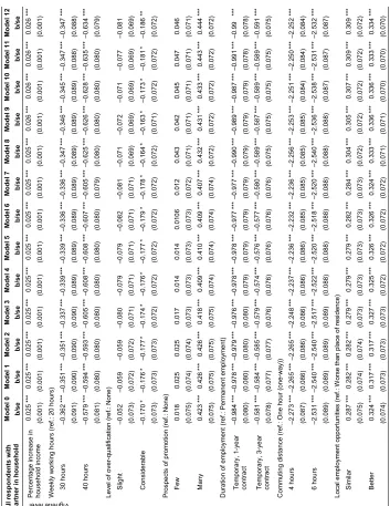
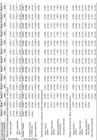
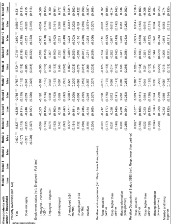
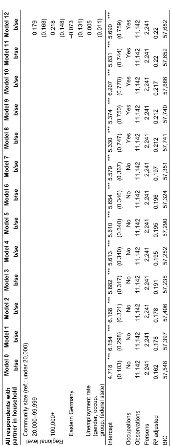
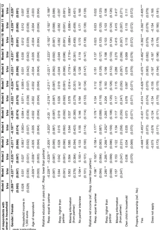
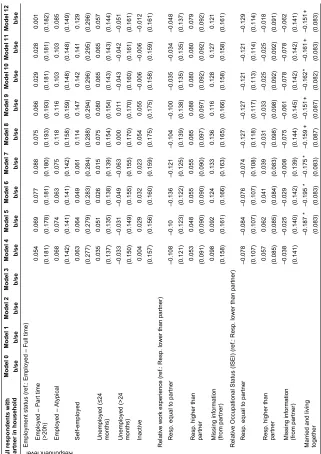
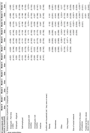
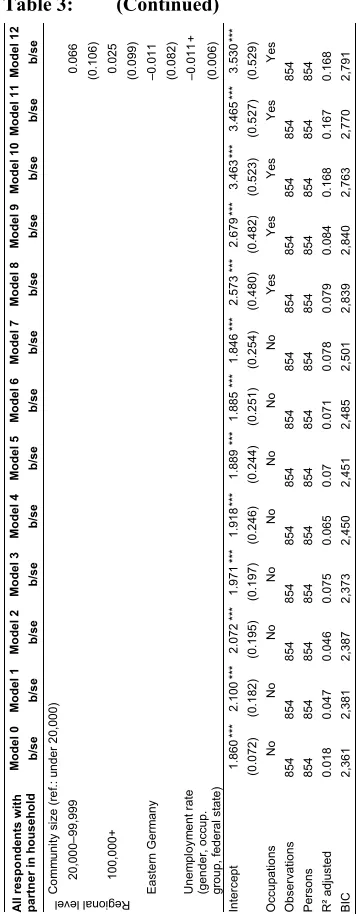
For all hypotheses, we discuss results from the PASS dataset for respondents with partners inside the household, first for the acceptance evaluation of the vignette job offer (Table 2), then for the general willingness to relocate for a job offer (Table 3), and third for the actual applications to interregional vacancies (Table 4). Tables A-3 to A-5 in the Appendix contain the corresponding models for respondents without partners.

While all CAPI respondents that were available to the labor market, in general, underwent the factorial survey experiment, only respondents that were searching for jobs within the last four weeks received the questions about their general willingness and their actual interregional applications, which led to different sample sizes but also had conceptual implications. The factorial survey experiment (Table 2 and Table A-3) in effect standardizes the labor-demand side and eliminates the selectivity found in real labor markets, which should allow the identification of causal estimates of job offer characteristics but should also aid in observing the effects of job characteristics on respondent-level variables (e.g., gender) over a fuller range than what is normally found in the labor market. Our other two dependent variables were restricted to respondents who actually looked for a job and could, therefore, be expected to have grappled with the decision about regional mobility and, thus, represent a more informed group. The question of willingness to relocate for a job (Table 3 and Table A-4) did not provide any information about the job itself and was, therefore, an indicator of general willingness to relocate. The question about the number of interregional applications (Table 4 and Table A-5) asked for actual behavior, rather than hypothetical concessions, and thus brought in another perspective. Together, these indicators offer a unique perspective on gender-specific willingness to move.

(18)

Table 2: Acceptance of vignette job offer

A

ll respo

ndents with

partner in h

ousehold Model 0 Model 1 Model 2 Model 3 Model 4 Model 5 Model 6 Model 7 Model 8 Model 9 Model 1 0 Model 1 1 Model 1 2 b/se b/se b/se b/s e b/se b/se b/se b/se b/se b/se b/se b/se b/s e Vignette level Percenta

ge increase in

house hold inc om e 0.025 ** * 0.025 ** * 0.025 ** * 0.025 ** * 0.025 ** * 0.025 ** * 0.025 ** * 0.025 ** * 0.025 ** * 0.026 ** * 0.026 ** * 0.026 ** * 0.026 ** * (0.0 01) (0.0 01) (0.0 01) (0.0 01) (0.0 01) (0.0 01) (0.0 01) (0.0 01) (0.0 01) (0.0 01) (0.0 01) (0.0 01) (0.0 01) W eek ly w orking hours

(ref.: 20 hours)

30 ho urs –0.36 2 ** * –0.35 1 ** * –0.35 1 ** * –0.33 7 ** * –0.33 9 ** * –0.33 9 ** * –0.33 6 ** * –0.33 6 ** * –0.34 7 ** * –0.34 6 ** * –0.34 5 ** * –0.34 7 ** * –0.34 7 ** * (0.0 91) (0.0 90) (0.0 90) (0.0 90) (0.0 89) (0.0 89) (0.0 89) (0.0 89) (0.0 89) (0.0 89) (0.0 89) (0.0 88) (0.0 88) 40 ho urs –0.57 9 ** * –0.59 4 ** * –0.59 3 ** * –0.60 5 ** * –0.60 8 ** * –0.60 8 ** * –0.60 7 ** * –0.60 5 ** * –0.62 5 ** * –0.62 6 ** * –0.62 8 ** * –0.63 5 ** * –0.63 4 ** * (0.0 81) (0.0 80) (0.0 80) (0.0 80) (0.0 80) (0.0 80) (0.0 80) (0.0 79) (0.0 80) (0.0 80) (0.0 80) (0.0 80) (0.0 79) Level o f over -qua lifi cation (ref.: None) Sligh t –0.05 2 –0.05 9 –0.05 9 –0.08 0 –0.07 9 –0.07 9 –0.08 2 –0.08 1 –0.07 1 –0.07 2 –0.07 1 –0.07 7 –0.08 1 (0.0 73) (0.0 72) (0.0 72) (0.0 71) (0.0 71) (0.0 71) (0.0 71 ) (0.0 71) (0.0 69) (0.0 69) (0.0 69) (0.0 69) (0.0 69) Consi dera bl e –0.17 0 * –0.17 6 * –0.17 7 * –0.17 4 * –0.1 76 * –0.17 7 * –0.17 9 * –0.1 78 * –0.16 4 * –0.16 3 * –0.17 3 * –0.18 1 * –0.1 86 ** (0.0 73) (0.0 73) (0.0 73) (0.0 72) (0.0 72) (0.0 72) (0.0 72) (0.0 72) (0.0 72) (0.0 71) (0.0 72) (0.0 72) (0.0 72) Prospects of prom oti on (ref.: None) Few 0.018 0.025 0.025 0.017 0.014 0.014 0.010 6 0.012 0.043 0.042 0.045 0.047 0.046 (0.0 75) (0.0 74) (0.0 74) (0.0 73) (0.0 73) (0.0 73) (0.0 73) (0.0 72) (0.0 71) (0.0 71) (0.0 71) (0.0 71) (0.0 71) Many 0.423 ** * 0.426 ** * 0.426 ** * 0.418 ** * 0.409 ** * 0.410 ** * 0.409 ** * 0.407 ** * 0.432 ** * 0.431 ** * 0.433 ** * 0.443 ** * 0.444 ** * (0.0 75) (0.0 75) (0.0 75) (0.0 75) (0.0 74) (0.0 74) (0.0 74) (0.0 74) (0.0 72) (0.0 72) (0.0 72) (0.0 72) (0.0 72) Duratio

n of em

pl oym ent (re f.: Perm anen t em p loym ent) Tem por ary, 1-ye ar contr act –0.98 4 ** * –0.97 8 ** * –0.97 9 ** * –0.97 6 ** * –0.97 8 ** * –0.97 8 ** * –0.97 7 ** * –0.97 7 ** * –0.99 0 ** * –0.98 9 ** * –0.98 7 *** –0.99 1 ** * –0.99 ** * (0.0 80) (0.0 80) (0.0 80) (0.0 80) (0.0 79) (0.0 79) (0.0 79) (0.0 79) (0.0 79) (0.0 79) (0.0 79) (0.0 78) (0.0 78) Tem por ary, 3-ye ar contr act –0.58 1 ** * –0.58 4 ** * –0.58 5 ** * –0.57 9 ** * –0.57 4 ** * –0.57 6 ** * –0.57 7 ** * –0.58 0 ** * –0.58 9 ** * –0.58 7 ** * –0.58 9 ** * –0.58 9 ** * –0.59 1 ** * (0.0 78) (0.0 77) (0.0 77) (0.0 76) (0.0 76) (0.0 76) (0.0 76) (0.0 76) (0.0 75) (0.0 75) (0.0 75) (0.0 75) (0.0 75) Co mm uti ng dista nce (re f.: One h our (on e-w ay)) 4 hou rs –2.27 3 ** * –2.26 5 ** * –2.26 5 ** * –2.24 8 ** * –2.23 7 ** * –2.23 6 ** * –2.23 2 ** * –2.23 6 ** * –2.25 6 ** * –2.25 3 ** * –2.25 1 ** * –2.25 0 ** * –2.25 2 ** * (0.0 87) (0.0 86) (0.0 86) (0.0 86) (0.0 86) (0.0 86) (0.0 85) (0.0 85) (0.0 85) (0.0 85) (0.0 84) (0.0 84) (0.0 84) 6 hou rs –2.53 1 ** * –2.54 0 ** * –2.54 0 ** * –2.51 7 ** * –2.52 2 ** * –2.52 0 ** * –2.51 8 ** * –2.52 0 ** * –2.54 0 ** * –2.53 6 ** * –2.53 8 ** * –2.53 1 ** * –2.53 2 ** * (0.0 89) (0.0 89) (0.0 89) (0.0 89) (0.0 88) (0.0 88) (0.0 88) (0.0 88) (0.0 88) (0.0 88) (0.0 87) (0.0 87) (0. 087) Local e m pl oym ent o ppor tunities (ref.: W

orse than pla

ce of res

(19)

Table 2: (Continued)

A

ll resp

ondents wi

th

partner in h

ousehold Model 0 Model 1 Model 2 Model 3 Model 4 Model 5 Model 6 Model 7 Model 8 Model 9 Model 1 0 Model 1 1 Model 1 2 b/se b/se b/se b/se b/se b/se b/se b/s e b/se b/se b/se b/se b/se Vignette level Di ffi cu

lty of f

inding adequ ate accomm odati on (ref.: Ve ry ea sy) W ith som e effo rt –0.21 4 ** –0.19 7 ** –0.19 7 ** –0.18 9 ** –0.19 9 ** –0.1 99 ** –0.20 1 ** –0.20 1 ** –0.20 7 ** –0.21 0 ** –0.21 5 ** –0.21 4 ** –0.21 2 ** (0.0 73) (0.0 72) (0.0 72) (0.0 72) (0.0 72) (0.0 72) (0.0 72) (0.0 72) (0.0 71) (0.0 71) (0.0 71) (0.0 71) (0.0 70) W ith considerable effor t –0.38 8 ** * –0.37 5 ** * –0.37 5 ** * –0.37 4 ** * –0.37 5 ** * –0.37 6 ** * –0.37 6 ** * –0.37 1 ** * –0.37 9 ** * –0.37 9 ** * –0.37 8 ** * –0.37 4 ** * –0.37 4 ** * (0.0 77) (0.0 76) (0.0 76) (0.0 75) (0.0 76) (0.0 76) (0.0 76) (0.0 75) (0.0 74) (0.0 74) (0.0 74) (0.0 74) (0.0 74) Respondent level Gender: F emale –0.55 3 ** * –0.55 5 ** * –0.55 6 ** * –0.52 8 ** * –0.40 7 ** –0.4 08 ** –0.43 8 ** –0.43 7 ** –0.35 8 * –0.36 1 * –0.34 3 * –0.30 8 * –0.30 7 * (0.1 02) (0.1 10) (0.1 11) (0.1 09) (0.1 28) (0.1 28) (0.1 33) (0.1 33) (0.1 46) (0.1 46) (0.1 45) (0.1 44) (0.1 44) Househol d incom e

in 1,000 euros

–0.07 2 + –0.05 5 + –0.05 4 + –0.01 4 –0.00 7 –0.00 7 –0.00 2 –0.00 3 0.001 0.002 0.002 0.005 0.004 (0.0 41) (0.0 30) (0.0 30) (0.0 11) (0.0 10) (0.0 10) (0.0 11) (0.0 11) (0.0 14) (0.0 14) (0.0 14) (0.0 14) (0.0 14)

Age of r

espondent –0.03 7 ** * –0.03 7 ** * –0.02 6 ** * –0.02 6 ** * –0.02 5 ** * –0.02 5 ** * –0.02 5 ** * –0.02 8 ** * –0.02 8 ** * –0.02 6 ** * –0.02 5 ** * –0.02 5 ** * (0.0 05) (0.0 05) (0.0 06) (0.0 06) (0.0 06) (0.0 06) (0.0 06) (0.0 06) (0.0 06) (0.0 06) (0.0 06) (0.0 06) Rel ative education in years

(ref.: Resp. low

(20)

A

ll respo

ndents wit

h

partner in h

ousehold Model 0 Model 1 Model 2 Model 3 Model 4 Model 5 Model 6 Model 7 Model 8 Model 9 Model 1 0 Model 1 1 Model 1 2 b/se b/se b/se b/s e b/se b/se b/se b/s e b/se b/se b/se b/se b/se Respondent level Proper ty ownersh ip (re f.: No) Yes –0.93 0 ** * –0.82 7 ** * –0.82 0 ** * –0.78 5 ** * –0.78 7 ** * –0.73 4 ** * –0.71 9 ** * –0.67 0 ** * –0.65 9 ** * –0.63 1 ** * (0.1 07) (0.1 13) (0.1 14) (0.1 15) (0.1 15) (0.1 18) (0.1 18) (0.1 18) (0.1 17) (0.1 18) Does no t apply –0.27 8 –0.23 5 –0.24 6 –0.25 9 –0.24 8 –0.28 5 –0.25 5 –0.26 3 –0.22 0 –0.21 5 (0.3 26) (0 .327) (0.3 27) (0.3 26) (0.3 26) (0.3 18) (0.3 22) (0.3 23) (0.3 15) (0.3 16) Em pl oym ent sta tus (re f.: Em pl oyed – Full tim e ) Em pl oyed – Part tim e (>20h) –0.08 4 –0.08 3 –0.12 0 –0.10 8 –0.08 0 –0.07 8 –0.05 3 –0.05 4 –0.06 0 (0.1 56) (0.1 56) (0.1 56) (0.1 55) (0.1 59) (0.1 58) (0.1 58) (0.1 58) (0.1 58) Em pl oyed – Atyp ica l 0.079 0.081 0.038 0.045 0.054 0.057 0.062 0.059 0.060 (0.1 63) (0.1 63) (0.1 63) (0.1 63) (0.1 63) (0.1 63) (0.1 62) (0.1 61) (0.1 61 ) Self -em pl oyed 0.142 0.138 0.089 0.091 0.246 0.252 0.281 0.269 0.272 (0.2 42) (0.2 42) (0.2 42) (0.2 42) (0.2 48) (0.2 48) (0.2 49) (0.2 48) (0.2 49) Unem pl oyed ( ≤ 24 m onth s) 0.470 * 0.471 * 0.335 + 0.321 0.352 + 0.356 + 0.328 0.334 + 0.33 4 + (0.1 91) (0.1 91) (0.2 00) (0.2 00) (0.2 03) (0.2 03) (0.2 03) (0.2 02) (0.2 02) Unem pl oyed ( >24 m onth s) 0.132 0.130 –0.06 6 –0.06 3 –0.07 6 –0.07 6 –0.11 6 –0.12 4 –0.12 2 (0.2 38) (0.2 38) (0.252) (0.2 52) (0.2 61) (0.2 61) (0.2 60) (0.2 59) (0.2 59) Inacti ve –0.19 4 –0.18 4 –0.24 9 –0.25 7 –0.26 6 –0.27 1 –0.27 4 –0.37 9 + –0.38 7 + (0.2 04) (0.2 05) (0.2 07) (0.2 07) (0.2 08) (0.2 09) (0.2 06) (0.2 07) (0.2 08) Rel ativ e w ork e xperie

nce (ref.: Resp. lower than partner)

Resp. eq ual to part ner –0.20 9 –0.21 2 –0.18 8 –0.21 3 –0.12 5 –0.10 4 –0.11 6 –0.08 1 –0.09 2 (0.1 77) (0.1 77) (0.1 76) (0.1 79) (0.1 83) (0.1 83) (0.1 82) (0.1 82) (0.1 85) Resp. hig her than part ner 0.031 0.028 0.012 0.009 –0.01 4 –0.02 2 –0.01 7 –0.01 3 –0.01 4 (0.1 40) (0.1 40) (0.1 41) (0.1 41) (0.1 43) (0.1 42) (0.1 43) (0.1 42) (0.1 42) Missi ng infor m ati on (fr om par tner ) 0.294 0.289 0.282 0.293 0.348 0.341 0.346 0.351 0.336 (0.2 55) (0.2 54) (0.2 53) (0.2 53) (0.2 56) (0.2 56) (0.2 53) (0.2 52) (0.2 52) Rel ative Occupationa

l Status (

ISEI)

(re

f.: Resp. lo

w

er than partner)

(21)

A

ll respo

ndents wit

h

partner in h

ouse hold Model 0 Model 1 Model 2 Model 3 Model 4 Model 5 Model 6 Model 7 Model 8 Model 9 Model 1 0 Model 1 1 Model 1 2 b/se b/s e b/se b/se b/se b/se b/s e b/se b/se b/se b/se b/se b/se Respondent level Em pl oym ent sta tus of par tner (ref.: Em pl

oyed – Full tim

e) Em pl oyed – Part tim e (>20h) 0.042 0.034 0.080 0.078 0.049 0.050 0.032 (0.1 90) (0.1 89) (0.1 91) (0.1 91) (0.1 88) (0.1 86) (0.1 87) Em pl oyed – Atyp ica l 0.009 0.014 0.065 0.053 0.076 0.062 0.062 (0.1 92) (0.1 92) (0.1 97) (0.1 96) (0.1 98) (0.1 98) (0.1 98) Self -em pl oyed 0.126 0.116 0.133 0.121 0.077 0.054 0.053 (0.2 75) (0.2 76) (0.2 72) (0.2 72) (0.2 67) (0.2 66) (0.2 67) Unem pl oyed ( ≤ 24 m onths) 0.428 + 0.416 + 0.35 5 0.335 0.360 0.320 0.313 (0.2 41) (0.2 41) (0.2 42) (0.2 42) (0.2 41) (0.2 41) (0.2 42) Unem pl oyed ( >24 m onths) 0.638 * 0.625 * 0.623 * 0.593 * 0.598 * 0.513 + 0.51 5 + (0.2 95) (0.2 95) (0.2 97) (0.2 96) (0.2 95) (0.2 93) (0.2 93) Inacti ve 0.299 0.293 0.249 0.233 0.227 0.152 0.150 (0.1 98) (0.1 98) (0.2 01) (0.2 00) (0.1 99) (0.1 99) (0.2 00) Confli ct w ith house hold

(ref.: Very rare or nev

er) Rarely 0.137 0.091 0.086 0.084 0.095 0.108 (0.1 58) (0.1 60) (0.1 60) (0.1 58) (0.1 57) (0.1 57) So m eti m es 0.020 0.042 0.029 0.034 0.054 0.066 (0.1 55) (0.1 58) (0.1 58) (0.1 57 ) (0.1 56) (0.1 56) Often 0.045 0.027 0.006 –0.04 6 –0.00 3 0.006 (0.2 20) (0.2 21) (0.2 22) (0.2 20) (0.2 18) (0.2 17) Very fre quent 0.664 0.709 0.688 0.638 0.694 0.692 (0.4 59) (0.4 59) (0.4 57) (0.4 45) (0.4 43) (0.4 44) Size

of social netw

(22)

A

ll respo

ndents wit

h

partner in h

ousehold

Model 0

Model 1

Model 2

Model 3

Model 4

Model 5

Model 6

Model 7

Model 8

Model 9

Model 1

0

Model 1

1

Model 1

2

b/se

b/s

e

b/se

Regional level

Co

mm

uni

ty si

ze

(re

f.: under 2

0,000)

20,00

0

–99,999

0.179 _(0.1

68)

100,0

00+

0.218 _(0.1

48)

Eastern

Germ

any

–0.07

3

(0.1

31)

Unem

pl

oy

m

ent r

ate

(gen

der, occup.

grou

p, federal state)

0.005 _(0.0

11)

Inter

cept

4.718

**

*

6.154

**

*

6.168

**

*

5.882

**

*

5.613

**

*

5.610

**

*

5.654

**

*

5.579

**

*

5.330

**

*

5.374

**

*

6.207

**

*

5.831

**

*

5.690

**

*

(0.1

83)

(0.2

98)

(0.3

21)

(0.3

17)

(0.3

40)

(0.3

40)

(0.3

46)

(0.3

67)

(0.7

47)

(0.7

50)

(0.7

70)

(0.7

44)

(0.7

59)

Occupatio

ns

No

Yes

Obser

vations

11,14

2

11,1

42

11,14

2

11,14

2

11,14

2

11,14

2

11,14

2

11,14

2

11,14

2

11,14

2

11,14

2

11,14

2

11,14

2

Persons

2,241

R² adjusted

0.162

0.178

0.191

0.195

0.196

0.197

0.212

0.217

0.22

BIC

57,54

8

57,3

97

57,40

6

57,23

5

57,28

2

57,29

0

57,32

4

57,35

1

57,74

1

57,74

0

57,68

6

57,65

2

57,68

2

Note: Cluste

r robust standard errors in parent

heses (

+ p<0.10, * p<0.05, ** p<0.01, ***

p<0.00

(23)

Table 3: Willingness to relocate for a hypothetical job offer

A

ll respo

ndents wit

h

partner in h

ousehold Model 0 Model 1 Model 2 Model 3 Model 4 Model 5 Model 6 Model 7 Model 8 Model 9 Model 1 0 Model 1 1 Model 1 2 b/se b/se b/se b/s e b/se b/se b/s e b/se b/s e b/s e b/se b/se b/s e Respondent level Gender: F emale –0.26 9 ** * –0.23 7 ** * –0.23 5 ** * –0.21 1 ** –0.19 7 ** –0.20 5 ** –0.22 2 ** –0.22 4 ** –0.23 3 * –0.2 31 * –0.23 9 ** –0.23 9 ** –0.22 9 * (0.0 65) (0.0 67) (0.0 67) (0.0 66 ) (0.0 74) (0.0 74) (0.0 76) (0.0 77) (0.0 96) (0.0 95) (0.0 91) (0.0 90) (0.0 91) Househol d incom e i n 1,000 euros 0.028 0.031 0.027 0.063 * 0.063 + 0.064 + 0.071 + 0.06 5 + 0.031 0.030 0.012 0.012 0.007 (0.0 29) (0.0 30) (0.0 31) (0.0 3 2) (0.0 37) (0.0 36) (0.0 38) (0.0 37) (0.0 42) (0.0 42) (0.0 39) (0.0 39) (0.0 40)

Age of r

espondent –0.00 9 ** –0.00 8 * –0.00 5 –0.00 5 –0.00 2 –0.00 2 –0.00 2 –0.00 4 –0.00 5 –0.00 4 –0.00 4 –0.00 3 (0.0 03) (0.0 03) (0.0 04) (0.0 04) (0.0 04) (0.0 04) (0.0 04) (0.0 04) (0.0 04) (0.0 04) (0.0 04) (0.0 04) Rel at ive educa tio

n in years

(ref.: Resp. low

er t

han p

artner)

Resp. eq

ual to partner

–0.22 8 ** –0.22 9 ** –0.20 5 * –0.2 03 * –0.20 * –0.21 8 * –0.2 11 * –0.22 1 * –0.2 23 * –0.19 2 * –0.19 2 * –0.18 8 * (0.0 87) (0.0 87) (0.0 85) (0.0 87) (0.0 87) (0.0 87) (0.0 87) (0.0 92) (0.0 92) (0.0 87) (0.0 88) (0.0 88) Resp. hig her than par tner 0.044 0.042 0.028 0.015 0.019 0.026 0.019 –0.04 9 –0.04 9 –0.08 2 –0.08 2 –0.09 7 (0.0 91) (0.0 91) (0.0 90) (0.0 92) (0.0 92) (0.0 92) (0.0 91) (0.0 96) (0.0 96) (0.0 91) (0.0 91) (0.0 91) Missi ng infor m ati on (fr om par tner ) 0.563 0.564 0.585 0.544 0.537 0.578 0.614 + 0.719 + 0.718 + 0.886 + 0.886 + 0.90 8 * (0.3 79) (0. 384) (0.3 94) (0.4 03) (0.3 80) (0.3 79) (0.3 51) (0.3 86) (0.3 81) (0.4 58) (0.4 59) (0.4 51) No par tner interview 0.194 + 0.193 + 0.133 0.155 0.146 0.164 0.167 0.128 0.119 0.170 0.171 0.165 (0.1 01) (0.1 01) (0.1 00) (0.1 14) (0.1 14) (0.1 33) (0.1 34) (0.1 47) (0.1 47) (0.1 38) (0.1 39) (0.1 39) Rel at ive net inco m e (re f.: Resp. low er t han pa rtne r) Resp. eq

ual to partner

(24)

A

ll respo

ndents wit

h

partner in h

ousehold Model 0 Model 1 Model 2 Model 3 Model 4 Model 5 Model 6 Model 7 Model 8 Model 9 Model 1 0 Model 1 1 Model 1 2 b/se b/se b/se b/s e b/se b/se b/s e b/se b/s e b/s e b/se b/se b/s e Respondent level Em pl oym ent sta tus (re f.: Em pl oyed – Full tim e ) Em pl oyed – Part tim e (>20h ) 0.054 0.069 0.077 0.088 0.075 0.066 0.029 0.028 0.001 (0.1 81) (0.1 78) (0.1 81) (0.1 80) (0.1 93) (0.1 93) (0.1 81) (0.1 81) (0.1 82) Em pl oyed – Atyp ica l 0.068 0.074 0.063 0.075 0.118 0.116 0.103 0.103 0.085 (0.1 42) (0.1 41) (0.1 41) (0.1 42) (0.1 58) (0.1 59) (0.1 48) (0.1 48) (0.1 49) Sel f-em pl oyed 0.063 0.064 0.049 0.061 0.114 0.147 0.142 0.141 0.129 (0.2 77) (0.2 79) (0.2 83) (0. 284) (0.2 88) (0.2 94) (0.2 96) (0.2 95) (0.2 96) Unem pl oyed ( ≤ 24 m onths) 0.035 0.051 0.026 0.015 0.075 0.080 0.065 0.065 0.057 (0.1 37) (0.1 35) (0.1 38) (0.1 39) (0.1 54) (0.1 54) (0.1 43) (0.1 43) (0.1 44) Unem pl oyed ( >24 m onths) –0.03 3 –0.03 1 –0.04 9 –0.06 3 0.000 0.011 –0.04 3 –0.04 2 –0.05 1 (0.1 50) (0.1 49) (0.1 55) (0.1 55) (0.1 70) (0.1 70) (0.1 60) (0.1 61) (0.1 61) Inacti ve 0.004 0.029 0.032 0.023 0.054 0.055 –0.00 6 –0.00 6 –0.01 2 (0.1 57) (0.1 56) (0.1 60) (0.1 59) (0.1 75) (0.1 75) (0.1 58) (0.1 59) (0.1 61) Rel at ive w ork e xperie nce (re

f.: Resp. lo

w

er than pa

rtner)

Resp. eq

ual to partner

–0.10 8 –0.10 –0.13 6 –0.12 1 –0.10 4 –0.10 0 –0.03 5 –0.03 4 –0.04 8 (0.1 21) (0.1 23) (0.1 22) (0.1 25) (0.1 39) (0.1 38) (0.1 35) (0.1 35) (0.1 37) Resp. hig her than par tner 0.053 0.048 0.055 0.055 0.085 0.088 0.080 0.080 0.079 (0.0 91) (0.0 90) (0.0 90) (0.0 90) (0 .097) (0.0 97) (0.0 92) (0.0 92) (0.0 92) Missi ng infor m ati on (fr om par tner ) 0.098 0.092 0.124 0.133 0.136 0.116 0.128 0.127 0.121 (0.1 58) (0.1 61) (0.1 66) (0.1 63) (0.1 65) (0.1 66) (0.1 58) (0.1 58) (0.1 61) Rel a tive Occupat io nal Status

(ISEI) (ref.: Res

p. l ow er t han partne r) Resp. eq

ual to partner

(25)

A

ll respo

ndents wit

h

partner in h

ousehold Model 0 Model 1 Model 2 Model 3 Model 4 Model 5 Model 6 Model 7 Model 8 Model 9 Model 1 0 Model 1 1 Model 1 2 b/se b/se b/se b/s e b/se b/se b/s e b/se b/s e b/s e b/se b/se b/s e Respondent level Em pl oym ent sta tus of par tner (ref.: Em pl

oyed – Full tim

e) Em pl oyed – Part tim e (>20h ) –0.05 3 –0.05 0 –0.05 6 –0.07 5 –0.08 9 –0.08 9 –0.08 5 (0.1 47) (0.1 46) (0.1 45) (0.1 46) (0.1 35) (0.1 35) (0.1 37) Em pl oyed – Atyp ica l 0.050 0.058 –0.00 8 –0.02 4 0.077 0.077 0.062 (0.1 23) (0.1 25) (0.1 32) (0.1 33) (0.1 27) (0.1 28) (0.1 29) Sel f-em pl oyed –0.01 6 –0.03 0 –0.11 4 –0.13 6 –0.19 8 –0.19 8 –0.19 8 (0.1 80) (0.1 78) (0.1 92) (0.1 94) (0.1 96) (0.1 96) (0.1 93) Unem pl oyed ( ≤ 24 m onths) 0.254 + 0.27 6 + 0.195 0.173 0.274 + 0.274 + 0.27 5 + (0.1 52) (0 .151) (0.1 62) (0.1 62) (0.1 52) (0.1 52) (0.1 52) Unem pl oyed ( >24 m onths) –0.04 9 –0.03 2 –0.10 1 –0.12 8 –0.00 8 –0.00 7 –0.00 3 (0.1 63) (0.1 64) (0.1 75) (0.1 75) (0.1 66) (0.1 66) (0.1 67) Inacti ve 0.043 0.058 0.024 0.003 0.047 0.047 0.037 (0.1 41) (0.1 40) (0.1 54) (0.1 56) (0.1 44) (0.1 45) (0.1 46) Confli ct w ith house hold

(ref.: Very rare or nev

(26)

A

ll respo

ndents wit

h

partner in h

ousehold

Model 0

Model 1

Model 2

Model 3

Model 4

Model 5

Model 6

Model 7

Model 8

Model 9

Model 1

0

Model 1

1

Model 1

2

b/se

b/s

e

b/se

b/s

e

b/se

b/s

e

b/se

Regional level

Co

mm

uni

ty si

ze

(re

f.: under 2

0,000)

20,00

0–99,999

0.066 _(0.1

06)

100,0

00+

0.025 _(0.0

99)

Eastern

Germ

any

–0.01

1

(0.0

82)

Unem

pl

oy

m

ent r

ate

(gen

der, occup.

grou

p, federal state)

–0.01

1

+

(0.0

06)

Inter

cept

1.860

**

*

2.100

**

*

2.072

**

*

1.971

**

*

1.918

**

*

1.889

**

*

1.885

**

*

1.846

**

*

2.573

**

*

2.679

**

*

3.463

**

*

3.465

**

*

3.530

**

*

(0.0

72)

(0.1

82)

(0.1

95)

(0.1

97)

(0.2

46)

(0.2

44)

(0.2

51)

(0.2

54)

(0.4

80)

(0.4

82)

(0.5

23)

(0.5

27)

(0.5

29)

Occupatio

ns

No

Yes

Obser

vations

854

Persons

854

R² adjusted

0.018

0.047

0.046

0.075

0.065

0.07

0.071

0.078

0.079

0.084

0.168

0.167

0.168

BIC

2,361

2,381

2,387

2,373

2,450

2,451

2,485

2,501

2,839

2,840

2,763

2,770

2,791

Note

: Robust

st

anda

rd er

ror

s

in pare

nthese

s

(+

p<0.10

, * p<0.05,

**

p<0.01

, ***

p<0.00

(27)

Table 4: Number of applications to interregional vacancies

A

ll respo

ndents wit

h

partner in h

ousehold Model 0 Model 1 Model 2 Model 3 Model 4 Model 5 Model 6 Model 7 Model 8 Model 9 Model 1 0 Model 1 1 Model 1 2 b/s e b/se b/se b/se b/se b/se b/se b/se b/se b/s e b/se b/se b/s e Respondent level Gender: F emale –0.22 3 * –0.21 8 * –0.21 7 * –0.2 21 * –0.37 1 ** * –0.37 1 ** * –0.39 7 ** * –0.39 6 ** * –0.29 7 * –0.2 98 * –0.30 2 * –0.34 8 ** –0.36 5 ** (0.0 95) (0.1 03) (0.1 05) (0.1 09) (0.1 06) (0.1 06) (0.1 09) (0.1 06) (0.1 29) (0.1 30) (0.1 28) (0.1 30) (0.1 40) Househol d incom e i n 1,000 euros 0.011 0.025 0.024 0.022 0.054 0.054 0.044 0.042 0.047 0.047 0.033 0.025 0.027 (0.0 33) (0.0 34) (0.0 34) (0.0 35) (0.0 42) (0.0 42) (0.0 43) (0.0 45) (0.0 50) (0.0 50) (0.0 48) (0.0 46) (0.0 46)

Age of r

espondent –0.00 3 –0.00 3 –0.00 4 –0.00 3 –0.00 3 –0.00 3 –0.00 3 –0.00 6 –0.00 7 –0.00 6 –0.00 6 –0.00 7 (0.0 05) (0.0 05) (0.0 05) (0.0 05) (0.0 05) (0.0 05) (0.0 05) (0.0 05) (0.0 06) (0.0 06) (0.0 06) (0.0 06) Rel at ive educa tio

n in years (ref.: Re

sp. low

er t

han p

artner)

Resp. eq

ual to partner

0.070 0.069 0.069 0.012 0.012 –0.00 5 –0.00 6 –0.01 4 –0.01 7 0.017 –0.01 5 –0.03 1 (0.1 12) (0.1 12) (0.1 13) (0.1 17) (0.1 17) (0.1 19) (0.1 21) (0.1 32) (0.1 32) (0.1 30) (0.1 29) (0.1 31) Resp. hig her than par tner 0.279 + 0.279 * 0.283 * 0.20 3 0.202 0.204 0.193 0.216 + 0.216 + 0.185 0.175 0.156 (0.1 44) (0.1 42) (0.1 42) (0.1 35) (0.1 34) (0.1 33) (0.1 32) (0.1 28) (0.1 28) (0.127) (0.1 28) (0.1 29) Missi ng infor m ati on (fr om par tner ) –0.27 0 ** –0.26 9 ** –0.27 8 ** –0.25 2 –0.25 1 –0.20 8 –0.15 0 0.032 0.029 0.178 0.144 0.175 (0.1 03) (0.1 03) (0.1 07) (0.1 71) (0.1 71) (0.1 58) (0.1 50) (0.1 90) (0.1 91) (0.2 62) (0.2 86) (0.2 96) No par tner interview 0.244 * 0.244 * 0.249 * 0.24 7 0.247 0.127 0.139 0.212 0.200 0.241 0.278 0.298 (0.1 22) (0.1 21) (0.1 18) (0.1 66) (0.1 68) (0.2 10) (0.2 06) (0.2 23) (0.2 21) (0.2 22) (0.2 26) (0.2 28) Rel at ive net inco m e (r ef.: Resp. low er t han pa rtne r) Resp. eq

ual to partner

0.220 + 0.219 + 0.220 0.357 * 0.358 * 0.487 * 0.48 6 * 0.591 ** 0.577 ** 0.481 * 0.518 * 0.522 * (0.1 33) (0.1 32) (0.1 34) (0.1 59) (0.1 59) (0.2 02) (0.2 02) (0.2 21 ) (0.2 19) (0.2 17) (0.2 17) (0.2 20) Resp. hig her than par tner 0.123 0.123 0.123 0.278 + 0.278 + 0.398 + 0.38 6 + 0.443 * 0.441 * 0.380 + 0.380 + 0.36 8 + (0.1 55) (0.1 55) (0.1 54) (0.1 67) (0.1 65) (0.2 29) (0.2 29) (0.2 05) (0.2 06) (0.2 01) (0.2 01) (0.2 06) Missi ng infor m ati on (fr om par tner ) –0.21 5* –0.21 5 * –0.21 8 * 0.07 9 0.080 0.088 0.083 0.145 0.126 0.265 0.255 0.212 (0.0 85) (0.0 87) (0.0 90) (0.1 33) (0.1 37) (0.1 56) (0.1 52) (0.1 85) (0.1 79) (0.1 93) (0.186) (0.1 92) Ow n chi ld in hou sehold 0.004 0.003 –0.01 8 –0.01 9 0.010 0.027 0.064 0.052 0.088 0.112 0.103 (0.0 86) (0.0 86) (0.0 84) (0.0 85) (0.0 92) (0.0 94) (0.1 05) (0.1 06) (0.1 06) (0.1 07) (0.1 08) Prope

rty ownership (ref

(28)

A

ll resp

ondents wi

th

partner in h

ousehold Model 0 Model 1 Model 2 Model 3 Model 4 Model 5 Model 6 Model 7 Model 8 Model 9 Model 1 0 Model 1 1 Model 1 2 b/se b/se b/se b/s e b/se b/se b/se b/se b/se b/se b/se b/se b/s e Respondent level Em pl oym ent sta tus ( ref. : Em pl oyed – Fu ll t im e ) Em pl oyed – Part tim e (>20h ) 0.523 0.523 0.505 0.503 0.397 + 0.387 0.413 + 0.39 6 + 0.428 + (0.3 98) (0.3 97) (0.3 59) (0.3 61) (0.2 36) (0.2 36) (0.2 37) (0.2 36) (0.2 40) Em pl oyed – Atyp ica l 0.219 * 0.219 * 0.220 * 0.230 * 0.180 0.182 0.198 0.203 0.207 (0. 109) (0.1 08) (0.1 09) (0.1 09) (0.1 28) (0.1 28) (0.1 32) (0.1 33) (0.1 42) Self -em pl oyed 0.740 * 0.740 * 0.671 * 0.690 * 0.727 * 0.752 * 0.784 * 0.740 * 0.783 * (0.2 90) (0.2 90) (0.2 98) (0.2 97) (0.3 30) (0.3 31) (0.3 24) (0.3 25) (0.3 30) Unem pl oyed ( ≤ 24 m onths) 0.460 ** * 0.460 ** * 0.508 ** * 0.486 ** * 0.444 ** 0.454 ** 0.474 ** 0.468 ** * 0.475 ** (0.1 38) (0.1 35) (0.1 40) (0.1 38) (0.1 38) (0.1 39) (0.1 44) (0.1 41) (0.1 48) Unem pl oyed ( >24 m onths) 0.139 0.139 0.220 0.202 0.185 0.200 0.179 0.213 0.215 (0.1 27) (0.1 27) (0.1 39) (0.1 35) (0.1 35) (0.1 36) (0.1 39) (0.1 43) (0.1 53) Inacti ve 0.500 + 0.499 + 0.547 + 0.535 + 0.530 0.536 + 0.522 0.604 + 0.624 + (0.2 84) (0.2 82) (0.2 85) (0.2 89) (0.3 24) (0.3 25) (0.3 17) (0.3 39) (0.3 46) Rel at ive w ork e xperie

nce (ref.: Resp. lower th

an pa

rtner)

Resp. eq

ual to partner

–0.42 7 ** –0.42 8 ** –0.43 5 ** –0.42 4 ** –0.37 5 * –0.36 7 * –0.30 1 + –0.28 6 + –0.31 4 + (0.1 40) (0.1 40) (0.1 40) (0.1 36) (0.1 56) (0.1 55) (0.1 60) (0.1 61) (0.1 67) Resp. hig her than part ner –0.26 5 + –0.26 5 + –0.25 0 –0.25 2 –0.13 4 –0.12 8 –0.13 1 –0.12 0 –0.10 2 (0.1 58) (0.1 58) (0.1 56) (0.1 55) (0.1 58) (0.1 57) (0.1 54) (0.1 55) (0.1 60) Missi ng infor m ati on (fr om par tner ) 0.132 0.133 0.139 0.138 0.231 0.209 0.230 0.233 0.242 (0.2 44) (0.2 45) (0.2 51) (0.2 47) (0.2 35) (0.2 38) (0.2 33) (0.230) (0.2 37) Rel at ive Occupat io nal Status

(ISEI) (ref.: Res

p. l ow er t han partne r) Resp. eq

ual to partner

(29)

A

ll respo

ndents wit

h

partner in h

ousehold Model 0 Model 1 Model 2 Model 3 Model 4 Model 5 Model 6 Model 7 Model 8 Model 9 Model 1 0 Model 1 1 Model 1 2 b/se b/se b/se b/se b/se b/se b/se b/se b/se b/se b/se b/se b/s e Em pl oym ent sta tus of par

tner (ref.: Em

pl oyed – Full tim e) Em pl oyed – Part tim e (>20h ) –0.16 0 –0.15 1 –0.10 5 –0.13 0 –0.11 6 –0.11 6 –0.11 9 (0.1 67) (0.1 65) (0.1 73) (0.1 74) (0.1 73) (0.1 74) (0.1 76) Em pl oyed – Atyp ica l –0.28 5 * –0.2 59 + –0.38 8 * –0.40 3 * –0.32 2 * –0.30 0 + –0.29 3 + (0.1 39) (0.1 39) (0.1 56) (0.1 56) (0.1 60) (0.1 58) (0.1 59) Self -em pl oyed 0.535 0.547 0.430 0.406 0.341 0.322 0.363 (0.7 16) (0.6 90) (0.5 09) (0.5 10) (0.4 99) (0.4 98) (0.4 99) Unem pl oyed ( ≤ 24 m onths) –0.13 8 –0.11 3 –0.22 9 –0.25 6 –0.18 0 –0.15 9 –0.14 2 (0.2 16) (0.2 18) (0.2 14) (0.2 12) (0.2 10) (0.2 10) (0.2 17) Unem pl oyed ( >24 m onths) –0.51 8 * –0.4 95 * –0.64 9 ** –0.68 4 ** –0.58 8 * –0.53 4 * –0.5 35 * (0.2 04) (0.2 03) (0.2 49) (0.2 50) (0.2 48) (0.2 45) (0.2 47) Inacti ve –0.30 1 –0.27 6 –0.33 2 –0.35 8 + –0.32 9 –0.30 3 –0.31 4 (0.1 99) (0.2 02) (0.2 20) (0.2 17) (0.2 18) (0.2 16) (0.2 20) Confli ct w ith house hold (ref.:

Very rare or

never) Rarely –0.07 0 –0.10 9 –0.10 6 –0.09 9 –0.11 2 –0.10 7 (0.1 45) (0.1 49) (0.1 48) (0.1 44) (0.1 43) (0.1 44) So m eti m es –0.17 9 –0.27 3 * –0.26 9 * –0.26 1 * –0.28 2 * –0.2 80 * (0.1 24) (0.1 35) (0.1 34) (0.1 31) (0.1 29) (0.1 28 ) Often 0.002 –0.14 8 –0.16 6 –0.16 6 –0.20 0 –0.20 9 (0.2 42) (0.1 88) (0.1 91) (0.1 89) (0.1 93) (0.1 93) Very fr equent 0.148 0.140 0.124 0.029 –0.03 1 –0.02 9 (0.3 35) (0.3 73) (0.3 73) (0.3 46) (0.3 51) (0.3 40) Size

of social netw

(30)

A

ll respo

ndents with

partner in h

ousehold

Model 0

Model 1

Model 2

Model 3

Model 4

Model 5

Model 6

Model 7

Model 8

Model 9

Model 1

0

Model 1

1

Model 1

2

b/s

e

b/se

b/s

e

b/se

b/s

e

b/se

b/s

e

Regional level

Co

mm

uni

ty

si

ze (ref.: und

er 2

0,000)

20,00

0–99,999

–0.13

5

(0.2

40)

100,0

00+

–0.33

0

(0.2

07)

Eastern

Germ

any

0.074 _(0.1

20)

Unem

pl

oy

m

ent r

ate

(gen

der, occup. group,

feder

al

st

ate)

–0.01

7

*

(0.0

08)

Inter

cept

0.407

**

*

0.301

0.297

0.322

0.000

0.001

0.106

0.179

–0.17

3

–0.04

6

0.601

+

0.973

*

1.183

*

(0.0

98)

(0.2

24)

(0.2

30)

(0.2

42)

(0.3

02)

(0.2

96)

(0.3

12)

(0.3

15)

(0.3

29)

(0.3

41)

(0.3

55)

(0.4

23)

(0.4

93)

Occupatio

ns

No

Yes

Obser

vations

929

Persons

929

R² adjusted

0.004

0.003

0.001

0.018

0.017

0.023

0.021

0.034

0.037

0.065

0.077

0.083

BIC

3,373

3,419

3,426

3,4

39

3,493

3,500

3,529

3,554

3,892

3,896

3,874

3,868

3,884

Note

: Robust

st

anda

rd er

ror

s

in pare

nthese

s

(+

p<0.10

, * p<0.05,

**

p<0.01

, ***

p<0.00