ISSN: 2008-6822 (electronic)
http://dx.doi.org/10.22075/ijnaa.2017.1860.1485
An inexact alternating direction method with SQP
regularization for the structured variational
inequalities
Abdellah Bnouhachema,∗, Themistocles M. Rassiasb
a Ibn Zohr University, ENSA, BP 1136, Agadir, Morocco
bDepartment of Mathematics, National Technical University of Athens Zografou Campus 157 80, Athens, Greece
(Communicated by M. Eshaghi)
Abstract
In this paper, we propose an inexact alternating direction method with square quadratic proximal (SQP) regularization for the structured variational inequalities. The predictor is obtained via solving SQP system approximately under significantly relaxed accuracy criterion and the new iterate is computed directly by an explicit formula derived from the original SQP method. Under appropriate conditions, the global convergence of the proposed method is proved. We show theO(1/t) convergence rate for the inexact SQP alternating direction method. We also reported some numerical results to illustrate the efficiency of the proposed method.
Keywords: Variational inequalities; monotone operator; square quadratic proximal method;
logarithmic-quadratic proximal method; alternating direction method.
2010 MSC: Primary 90C33; Secondary 49J40.
1. Introduction
LetR stand for the real axis; and Rn
+ ={x ∈R;x≥0},Rn++ ={x∈R;x >0}, denote the positive half-axis and strict positive half-axis, respectively.
Further, givenn ∈N,put
Rn+ ={x= (x1, . . . , xn)>;x1, . . . , xn∈R+}
∗Corresponding author
Email addresses: [email protected](Abdellah Bnouhachem),[email protected](Themistocles M. Rassias)
and
Rn++={x= (x1, . . . , xn)>;x1, . . . , xn∈R++} where (.)> denotes the transpose.
Finally, define
Ω :=(u, v)>;u∈Rn
+, v ∈Rm+, A1u+A2v =b
where A1 ∈Rl×n, A2 ∈Rl×m, b∈Rl are given matrices and vectors, respectively. Consider the variational inequality problem:
find x∈Ω such that
(x0−x)>F(x)≥0, ∀x0 ∈Ω, (1.1) where
F(x) = (f1(u), f2(v))>. (1.2)
and f1 : Rn+ → Rn, f2 : Rm+ → Rm are given monotone operators. Studies and applications of such problems can be found in [14, 18, 19, 20, 21]. By attaching a Lagrange multiplier vector λ ∈ Rl to the linear constraints A
1u+A2v =b, the problem (1.1)+(1.2) may be expressed as find z ∈ Z0 :=
Rn+×Rm+ ×Rl such that
(z0−z)>Q(z)≥0, ∀z0 ∈ Z0, (1.3) where
z = (u, v, λ)>, Q(z) = f1(u)−A>1λ, f2(v)−A>2λ, A1u+A2v−b
>
. (1.4)
Various methods have been suggested to find the solution of problem (1.3)+(1.4). A popular approach is the alternating direction method (ADM) which was proposed by Gabay and Mercier [18] and Gabay [19]. Typically, problems in applications for example, network economics [32] and nonlinear mechanics [17, 20, 21] are quite large and are often solved by ADM. The ADM can reduce the scale of variational inequalities by decomposing the original problem into a series of subproblems with a lower scale (see [11, 20, 21, 27, 29, 37], for example). The classical proximal alternating directions method (PADM) is one of the attractive ADMs. From a given (uk, vk, λk)∈
Rn+×Rm+×Rl, the new iterate (uk+1, vk+1, λk+1) is obtained via solving the following problem
(u0 −u)>f1(u)−A>1[λ
k−β(A
1u+A2vk−b)] +r(u−uk) ≥0, ∀ u0 ∈Rn+, (1.5a) (v0−v)>f2(v)−A>2[λk−β(A1uk+1+A2v−b)] +s(v−vk) ≥0, ∀ v0 ∈Rm+, (1.5b) λk+1 =λk−β(A1u+A2v−b). (1.5c) Here r > 0, s > 0 are given proximal parameters and β > 0 is a given penalty parameter for the linearly constrained equation A1u +A2v −b = 0. Several works have been concentrated on the generalization of the proximal algorithm replacing in the alternating directions method (1.5a)-(1.5b) the proximal term r(u− uk) and s(v − vk) by some nonlinear functionals. Very recently, some alternating direction methods with logarithmic-quadratic proximal regularization [3, 4, 5, 6, 7, 8, 9, 30, 36, 39] have been developed by substituting in the alternating directions method (1.5a)-(1.5b) the term r(u−uk) and s(v−vk) by R[(u−uk) +µ(uk−U2
ku
−1)] and S[(v −vk) +µ(vk−V2 kv
−1)],
respectively. The predictor ˜zk = (˜uk,v˜k,w˜k,˜λk) in [3, 4, 5, 6, 7, 10, 30, 36, 39] is obtained via the following procedure: From a givenzk = (uk, vk, λk)∈
Rn++×Rm++×Rl, and µ∈(0,1), (˜uk,v˜k,λ˜k) is obtained via solving the following system:
f1(u)−A>1
λk−H(A1u+A2vk−b)
f2(v)−A>2
λk−H(A1u+A2v−b)
+S(v−vk) +µ(vk−Vk2v−1)= 0, (1.6b) λk+1 =λk−H(A1uk+A2vk−b), (1.6c) where H∈Rl×l, R∈
Rn×n, and S ∈Rm×m are symmetric positive definite matrices.
Define
Ω :=(u, v, w)> : u∈Rn1
+, v ∈R n2
+, w ∈R n3
+, A1u+A2v+A3w=b ,
where A1 ∈Rm×n1, A2 ∈Rm×n2, A3 ∈Rm×n3, b∈Rm are given matrices and vectors, respectively. In this paper, we consider the following structured variational inequality with three separable oper-ators: find y∈Ω such that
(y0−y)>F(y)≥0, ∀y0 ∈Ω, (1.7) where
F(y) = (f1(u), f2(v), f3(w)) >
, (1.8)
and f1 : Rn+1 → Rn1, f2 : R+n2 → Rn2, f3 : Rn+3 → Rn3 are given monotone operators. By attaching a Lagrange multiplier vector λ ∈ Rm to the linear constraints A
1u+A2v+A3w = b, the problem (1.7)+(1.8) can be explained in terms of finding z ∈ Z :=Rn1
+ ×R n2
+ ×R n3
+ ×Rm such that
(z0−z)>Q(z)≥0, ∀z0 ∈ Z, (1.9) where
z = (u, v, w, λ)>, Q(z) = f1(u)−A>1λ, f2(v)−A>2λ, f3(w)−A>3λ, A1u+A2v +A3w−b
>
. (1.10) The problem (1.9)+(1.10) is referred to as SVI3.
By combining the ADM and parallel splitting augmented Lagrangian method [33], Cao et al. [12] proposed a new partial splitting augmented Lagrangian method for solving SVI3. The predictor ˜zk= (˜uk,v˜k,w˜k,λ˜k) in [12] is obtained via the following procedure: From a givenzk = (uk, vk, wk, λk)∈ Z, (˜uk,v˜k,w˜k,λ˜k) is obtained via solving the following system:
(u−u˜k)>(f1(˜uk)−A>1[λ
k−βH(A
1u˜k+A2vk+A3wk−b)])≥0, ∀u∈Rn+1, (1.11a) (v−v˜k)>(f1(˜vk)−A>2[λk−βH(A1u˜k+A2v˜k+A3wk−b)])≥0, ∀v ∈Rn+2, (1.11b) (w−w˜k)>(f3( ˜wk)−A>3[λ
k−βH(A
1u˜k+A2vk+A3w˜k−b)])≥0, ∀w∈Rn+3, (1.11c) ˜
λk =λk−βH(A1u˜k+A2˜vk+A3w˜k−b). (1.11d) In this paper, we suggest that the complementarity subproblems arising in ADM (1.11a)-(1.11d) could be regularized by the square quadratic proximal (SQP) regularization, the SQP regularization forces the solutions of ADM subproblems to be interior points of Rn1
+, Rn+2 and Rn+3, respectively; thus the complementarity subproblems (1.11a), (1.11b) and (1.11c) reduce to three easier systems of nonlinear equations. More specifically, the iterative scheme of ADM with SQP regularization is as follows: From a givenzk = (uk, vk, wk, λk)∈
Rn++1 ×R++n2 ×Rn++3 ×Rm, (˜uk,v˜k,w˜k,λ˜k) is obtained via solving the following system:
f1(u)−A>1[λk−βH(A1u+A2v+A3w−b)] +R1[ 1 2(u−u
k
) +µ(uk−Uk(√u)−1)] = 0, (1.12a)
f2(v)−A>2[λ
k−βH(A
1u+A2v+A3w−b)] +R2[ 1 2(v −v
k) +µ(vk−V k(
√
f3(w)−A>3[λ
k−βH(A
1u+A2v+A3w−b)] +R3[ 1
2(w−w
k) +µ(wk−W k(
√
w)−1))] = 0, (1.12c)
˜
λk =λk−βH(A1u˜k+A2v˜k+A3w˜k−b),
where µ ∈ (0,1) and β > 0 are given constants; H ∈ Rm×m, R1 ∈ Rn1×n1, R2 ∈ Rn2×n2 and R3 ∈ Rn3×n3 are positive definite diagonal matrices; Uk, Vk and Wk are positive definite diagonal matrices defined by
Uk =diag(uk1
q
uk 1, . . . , u
k n
p
uk n) :=
uk 1
p
uk 1
. ..
uknpuk n
,
Vk =diag(v1k
q
vk 1, . . . , v
k n
p
vk n) and
Wk=diag(wk1
q
wk
1, . . . , wkn
p
wk n), (√u)−1 ∈ Rn1
++ is a vector whosej-th element is 1/
√
uj,(
√
v)−1 ∈ Rn2
++is a vector whosej-th element is 1/√vj, (
√
w)−1 ∈ Rn3
++ is a vector whose j-th element is 1/
√
wj.
Since (1.12a)–(1.12c) include both square and quadratic terms, the method is called the Square-Quadratic Proximal (SQP) method, and (1.12a), (1.12b) and (1.12c) are called the SQP system of nonlinear equations (SQP system).
By combining the ADM and SQP method, we propose an inexact alternating direction method for SVI3. Each iteration of the proposed method contains a prediction and a correction, the predictor is obtained via solving the SQP system approximately under significantly relaxed accuracy criterion and the new iterate is computed directly by an explicit formula derived from the original SQP method. We also study the global convergence of the proposed method under certain conditions. Our results can be viewed as significant extensions of the previously known results.
2. Inexact SQP alternating direction method
In this section, we suggest and consider the inexact SQP alternating direction method for solving SVI3.First, for any vectoru∈Rn,kuk∞= max{|u1|. . . ,|un|}.LetD∈Rn×nbe a symmetry positive definite matrix, we denote the D-norm of uby kuk2
D =uTDu. we make the following standard assumptions.
Assumption 2.1. f1 is monotone with respect to Rn+1, that is, (f1(x)−f1(y))T(x−y)≥0,∀x, y ∈
Rn+1, f2 is monotone with respect to R+n2 and f3 is monotone with respect to Rn+3. Assumption 2.2. The solution set of SVI3, denoted by Z∗, is nonempty.
Now, we are ready to present the inexact SQP alternating direction method for solving SVI3.
Algorithm 2.1.
Prediction step: For a given zk= (uk, vk, wk, λk)∈
Rn++1 ×R n2
++×R n3
++×Rm, µ∈(0,1) and β >0, the predictor ˜zk = (˜uk,v˜k,w˜k,λ˜k) ∈
Rn++1 ×Rn++2 ×Rn++3 ×Rm is obtained via solving the following system:
f1(u)−A>1[λk−βH(A1u+A2v+A3w−b)] +R1[ 1 2(u−u
k) +µ(uk−U k(
√
f2(v)−A>2[λ
k−βH(A
1u+A2v+A3w−b)] +R2[ 1 2(v−v
k) +µ(vk−V k(
√
v)−1)] =: ξvk ≈0, (2.1b)
f3(w)−A>3[λ
k−βH(A
1u+A2v+A3w−b)]+R3[ 1 2(w−w
k)+µ(wk−W k(
√
w)−1))] =:ξwk ≈0, (2.1c) ˜
λk=λk−βH(A1u˜k+A2v˜k+A3w˜k−b), (2.1d) where H∈Rm×m, R
1 ∈Rn1×n1, R2 ∈Rn2×n2 and R3 ∈Rn3×n3 and
kG−1ξkk2 G≤
1−µ 1 +µη
2kzk−z˜kk2
G, η∈(0,1), (2.2)
ξk =
ξk u ξk v ξwk 0 (2.3) and G= (1+µ) 2 R1
(1+µ) 2 R2
(1+µ) 2 R3
1 βH −1 . (2.4)
Correction step: The new iteratezk+1(αk) = (uk+1, vk+1, wk+1, λk+1) is the solution of the following system:
1−µ
1 +µαk[f1(˜u
k)−A> 1λ˜
k] +R 1[
1 2(u−u
k) +µ(uk−U k(
√
u)−1)] = 0, (2.5a)
1−µ
1 +µαk[f2(˜v
k)−A> 2λ˜
k] +R 2[
1 2(v−v
k) +µ(vk−V k(
√
v)−1)] = 0, (2.5b)
1−µ
1 +µαk[f3( ˜w
k)−A> 3λ˜
k] +R 3[
1
2(w−w
k) +µ(wk−W k(
√
w)−1)] = 0, (2.5c)
λk+1 =λk− 1−µ
1 +µαkβH(A1u˜ k
+A2v˜k+A3w˜k−b), (2.5d) where
αk=
ϕ(zk,z˜k)
kd(zk,z˜k)k2 G
, (2.6)
ϕ(zk,z˜k) := 1 2ku
k− ˜
ukk2R1+1 2kv
k− ˜
vkk2R2+1 2kw
k− ˜
wkk2R3+1 βkλ
k−˜
λkk2H−1+(zk−z˜k)>ξk (2.7)
and
d(zk,z˜k) :=zk−z˜k+G−1ξk. (2.8) Remark 2.1. The proposed method can be viewed as a prediction-correction method which uses the SQP systems in both the prediction and correction steps.
The main task of the prediction is to find an approximate solution of the following equations
f1(u)−A>1[λk−βH(A1u+A2v+A3w−b)] +R1[ 1 2(u−u
k
) +µ(uk−Uk(√u)−1)] = 0, (2.9a)
f2(v)−A>2[λk−βH(A1u+A2v+A3w−b)] +R2[ 1 2(v−v
k) +µ(vk−V k(
√
f3(w)−A>3[λ
k−βH(A
1u+A2v+A3w−b)] +R3[ 1
2(w−w
k) +µ(wk−W k(
√
w)−1)] = 0. (2.9c)
The exact solution of
f1(uk)−A>1[λ
k−βH(A
1uk+A2vk+A3wk−b)] +R1[ 1
2(u−u
k) +µ(uk−U k(
√
u)−1)] = 0 (2.10)
denoted by ˜uk, as the approximate solution of (2.9a). The exact solution of
f2(vk)−A>2[λ
k−βH(A
1u˜k+A2vk+A3wk−b)] +R2[ 1 2(v−v
k) +µ(vk−V k(
√
v)−1)] = 0 (2.11)
denoted by ˜vk, as the approximate solution of (2.9b). Then the exact solution of
f3(wk)−A3>[λk−βH(A1u˜k+A2˜vk+A3wk−b)] +R3[ 1
2(w−w
k) +µ(wk−W k(
√
w)−1)] = 0 (2.12)
denoted by ˜wk, as the approximate solution of (2.9c). It follows from (2.1) and (2.10)- (2.12) that
ξk =
ξuk ξvk ξk w 0
=
f1(˜uk)−f1(uk) +βA>1HA1(˜uk−uk) +βA>1HA2(˜vk−vk) +βA>1HA3( ˜wk−wk) f2(˜vk)−f2(vk) +βA>2HA2(˜vk−vk) +βA>2HA3( ˜wk−wk)
f3( ˜wk)−f3(wk) +βA>3HA3( ˜wk−wk) 0
.
We need the following result to study the convergence analysis of the proposed method.
Lemma 2.2. Let q(u)∈Rn be a monotone mapping of u with respect to
Rn+ and R :=diag(r1, . . . , rn)∈Rn×n
be a positive definite diagonal matrix. For a given uk >0, µ >0, if
Uk :=diag(uk1
q
uk 1, . . . , u
k n
p
uk n),
√
u= (√u1, . . . ,
√
un),
and (√u)−1 be an n-vector whose j-th element is 1/√uj, then the equation
q(u) +R[1 2(u−u
k) +µ(uk−U k(
√
u)−1)] = 0 (2.13)
has a unique positive solution u. Moreover, for any v ≥0, we have
(v−u)>q(u)≥ 1+µ4 ku−vk2
R− kuk−vk2R
+1−µ4 kuk−uk2
R. (2.14)
Proof . The proof of the first assertion is similar as Proposition 2 in [1]; hence it is omitted. We now prove the second assertion. For each t > 0, we have 12 1− 1
t
≤ 1− √1 t ≤
1
2(t−1), then we obtain after multiplication by vjukj ≥0 for each j = 1, . . . , n,
vjukj(1−
q
uk j
√
uj
)≤vjukj 1 2
uj uk j
−1
!
= 1
and after multiplication byujukj ≥0 for each j = 1, . . . , n,
−ujukj(1−
q
uk j
√
uj
)≤ujukj 1 2
ukj uj
−1
!
= 1 2u
k j(u
k
j −uj),
adding the two inequalities, then we obtained
(vj−uj)
1
2(uj−u k j) +µ
ukj −(
q
uk j)
3(√u j)−1
≤ 1
2µ(vj−u k
j)(uj−ukj) + 1
2(uj−u k
j)(vj−uj). Using the identities
1
2(vj −u k
j)(uj−ukj) = 1
4 (uj−u k j)
2−(u
j−vj)2+ (vj −ukj) 2
1
2(uj −u k
j)(vj −uj) = 1
4 (vj−u k j)
2−(v
j −uj)2−(uj−ukj) 2
and recalling (2.13), thus we obtained
(uj −vj)(−qj)≥rj
1 +µ
4 (uj−vj) 2−
(ukj −vj)2
+1−µ 4 (u
k j −uj)
2
.
Summing overj = 1, . . . , n, encountered (2.14). ut
3. Basic results
In this section, we prove some basic properties, which will be used to establish the sufficient and necessary conditions for the convergence of the proposed method. The following theorem explains the reason of choosing αk in the form (2.6).
Theorem 3.1. For given zk = (uk, vk, wk, λk) ∈ Rn1
++ × R n2
++ × R n3
++ × Rm, let zk+1(αk) = (uk+1, vk+1, wk+1, λk+1) be generated by (2.5a)-(2.5d). Then for any z∗ = (u∗, v∗, w∗, λ∗) ∈ Z∗, we
have
kzk−z∗k2
G− kzk+1(αk)−z∗k2G ≥ 1−µ
1 +µΦ(αk) (3.1)
where
Φ(αk) := 2αkϕ(zk,z˜k)−α2kkd(z k
,z˜k)k2G. (3.2)
Proof . Applying Lemma 2.2 to (2.1a), we get
(uk+1−u˜k)>
n
f1(˜uk)−A>1λk−βH(A1u˜k+A2v˜k+A3w˜k−b)]−ξuk
o
≥ 1+µ4 ku˜k−uk+1k2
R1 − ku
k−uk+1k2 R1
+ 1−µ4 kuk−u˜kk2
R1. (3.3)
Since
kuk−uk+1k2
R1 =ku
k−u˜kk2
R1 +ku˜
k−uk+1k2
R1 + 2(˜u
k−uk+1)>
Then
1 2(u
k+1−u˜k)>
R1(uk−u˜k) = 1 4
ku˜k−uk+1k2
R1 − ku
k−uk+1k2 R1
+ 1 4ku
k−u˜kk2
R1. (3.4)
Adding (3.3) and (3.4), we obtain
(uk+1−u˜k)>n(1 +µ) 2 R1(u
k−u˜k)−f
1(˜uk) +A>1λ˜ k+ξk
u
o
≤ µ
2ku
k−u˜kk2 R1,
which implies
2(1−µ) 1 +µ αk(u
k+1−u˜k)>n(1 +µ) 2 R1(u
k−u˜k)−f
1(˜uk) +A>1˜λ k+ξk
u
o
−1−µ
1 +µαkµku k−
˜
ukk2R1 ≤0.
(3.5)
Similarly, applying Lemma 2.2 to (2.1b), we get
(vk+1−v˜k)>f2(˜vk)−A>2[λk−βH(A1u˜k+A2v˜k+A3w˜k−b)]−ξvk
≥ 1+µ4 k˜vk−vk+1k2 R2 − kv
k−vk+1k2 R2
+1−µ4 kvk−˜vkk2
R2. (3.6)
Similar as (3.4), we have
1 2(v
k+1−v˜k)>
R2(vk−˜vk) = 1 4
k˜vk−vk+1k2 R2 − kv
k−vk+1k2 R2
+1 4kv
k−˜vkk2
R2. (3.7)
Adding (3.6) and (3.7), we have
(vk+1−v˜k)>
n(1 +µ)
2 R2(v k−
˜
vk)−f2(˜vk) +A>2λ˜k+ξvk
o
≤ µ
2kv k−
˜ vkk2R2, which implies
2(1−µ) 1 +µ αk(v
k+1−˜vk)>n(1 +µ) 2 R2(v
k−v˜k)−f
2(˜vk) +A>2λ˜ k+ξk
v
o
− 1−µ
1 +µαkµkv
k−˜vkk2 R2 ≤0.
(3.8)
Similarly, we have
2(1−µ) 1 +µ αk(w
k+1−w˜k)>n(1 +µ) 2 R3(w
k−w˜k)−f
3( ˜wk) +A>3˜λ k+ξk
w
o
−1−µ
1 +µαkµkw
k−w˜kk2 R3 ≤0.
(3.9)
We apply again Lemma 2.2 to (2.5a), we get
(uk+1−u∗)>−1−µ
1 +µαk[f1(˜u k
)−A>1λ˜k]
≥ 1+µ4 kuk+1−u∗k2
R1 − ku
k−u∗k2 R1
+1−µ4 kuk−uk+1k2
which implies
1 +µ 2
kuk−u∗k2
R1 − ku
k+1−u∗k2 R1
≥ 2(1−µ)
1 +µ αk(u
k+1−u∗
)>(f1(˜uk)−A>1λ˜
k) + 1−µ 2 ku
k−uk+1k2
R1. (3.11)
Similarly, applying Lemma 2.2 to (2.5b), we obtain
(vk+1−v∗)>−1−µ
1 +µαk[f2(˜v
k)−A> 2λ˜
k]
≥ 1+µ4 kvk+1−v∗k2 R2 − kv
k−v∗k2 R2
+ 1−µ4 kvk−vk+1k2
R2, (3.12)
which implies
1 +µ 2
kvk−v∗k2 R2 − kv
k+1−v∗k2 R2
≥ 2(1−µ)
1 +µ αk(v k+1−
v∗)>(f2(˜vk)−A>2λ˜ k
) + 1−µ 2 kv
k−
vk+1k2R2. (3.13) Similarly, we have
1 +µ 2
kwk−w∗k2
R3 − kw
k+1−w∗k2 R3
≥ 2(1−µ)
1 +µ αk(w
k+1−w∗
)>(f3( ˜wk)−A>3˜λk) + 1−µ
2 kw
k−wk+1k2
R3. (3.14)
On the other hand, from (2.5d), we have
kλk−λ∗k2
H−1 − kλk+1−λ
∗k2 H−1
=kλk−λk+1k2 H−1 +
2(1−µ) 1 +µ αkβ(λ
k+1−λ∗
)>(A1u˜k+A2v˜k+A3w˜k−b). (3.15) Since (u∗, v∗, w∗, λ∗) is a solution of SVI3, ˜uk ∈R++n1 , v˜k ∈R++n2 and ˜wk ∈Rn++3 , we have
(˜uk−u∗)>(f1(u∗)−A>1λ ∗
)≥0, (˜vk−v∗)>(f2(v∗)−A>2λ∗)≥0, ( ˜wk−w∗)>(f3(w∗)−A>3λ
∗ )≥0, and
A1u∗+A2v∗+A3w∗−b= 0. Using the monotonicity of f1, f2 and f3, we obtain
˜ uk−u∗ ˜ vk−v∗ ˜ wk−w∗
˜ λk−λ∗
>
f1(˜uk)−A>1λ˜k f2(˜vk)−A>2λ˜k f3( ˜wk)−A>3λ˜k A1u˜k+A2v˜k+A3w˜k−b
≥ ˜ uk−u∗
˜ vk−v∗ ˜ wk−w∗
˜ λk−λ∗
>
f1(u∗)−A>1λ ∗
f2(v∗)−A>2λ∗ f3(w∗)−A>3λ
∗
A1u∗ +A2v∗+A3w∗−b
≥0.
It follows from (3.11), (3.14)-(3.16) that
kzk−z∗k2 G− kz
k+1(α
k)−z∗k2G
≥ 1−µ
2 ku
k−uk+1k2 R1 +
1−µ 2 kv
k−vk+1k2 R2 +
1−µ 2 kw
k−wk+1k2 R3
+ 1 βkλ
k−λk+1k2 H−1 +
2(1−µ) 1 +µ αk(u
k+1−u˜k)>
(f1(˜uk)−A>1λ˜ k)
+2(1−µ) 1 +µ αk(v
k+1− ˜
vk)>(f2(˜vk)−A>2λ˜ k
)
+2(1−µ) 1 +µ αk(w
k+1−w˜k)>
(f3( ˜wk)−A>3λ˜ k)
+2(1−µ) 1 +µ αk(λ
k+1−λ˜k)>
(A1u˜k+A2v˜k+A3w˜k−b).
(3.17)
Adding (3.5), (3.8), (3.9) and (3.17), we get
kzk−z∗k2G− kzk+1(αk)−z∗k2G
≥ 1−µ
2 ku
k−uk+1k2 R1 +
1−µ 2 kv
k−vk+1k2 R2 +
1−µ 2 kw
k−wk+1k2 R3
+ 1 βkλ
k−λk+1k2 H−1 +
2(1−µ) 1 +µ αk(u
k+1−u˜k)>
(1 +µ) 2 R1(u
k−u˜k) +ξk u
+2(1−µ) 1 +µ αk(v
k+1−v˜k)>
(1 +µ) 2 R2(v
k−v˜k) +ξk v
+2(1−µ) 1 +µ αk(w
k+1−w˜k)>
(1 +µ) 2 R3(w
k−w˜k) +ξk w
+2(1−µ) 1 +µ αk(λ
k+1−˜
λk)>(A1u˜k+A2v˜k+A3w˜k−b)
−1−µ
1 +µαkµku
k−u˜kk2 R1 −
1−µ 1 +µαkµkv
k−v˜kk2 R2 −
1−µ
1 +µαkµkw
k−w˜kk2 R3
= 2(1−µ) 1 +µ αk(z
k+1
(αk)−z˜k)>G(zk−z˜k+G−1ξk) +1−µ
1 +µ
1 +µ
2 ku
k−uk+1k2 R1 +
1 +µ 2 kv
k−vk+1k2 R2
+1 +µ 2 kw
k−wk+1k2 R3 +
1 βkλ
k−λk+1k2 H−1
+ 2µ β(1 +µ)kλ
k−λk+1k2 H−1 −
1−µ 1 +µαkµku
k−u˜kk2 R1
−1−µ
1 +µαkµkv
k−˜vkk2 R2 −
1−µ
1 +µαkµkw
k−w˜kk2 R3
≥ 1−µ
1 +µkz k−
zk+1(αk)k2G+
2(1−µ) 1 +µ αk(z
k+1
(αk)−z˜k)>Gd(zk,z˜k)
−1−µ
1 +µαkµku
k−u˜kk2 R1 −
1−µ 1 +µαkµkv
k−v˜kk2 R2
−1−µ
1 +µαkµkw k−
˜ wkk2R3.
It follows from (3.18) that
kzk−z∗k2 G− kz
k+1(α
k)−z∗k2G
≥ 1−µ
1 +µ
kzk−zk+1(αk)k2G+ 2αk(zk+1(αk)−zk)>Gd(zk,z˜k) + 2αk(zk−z˜k)>Gd(zk,z˜k)−αkµkuk−u˜kk2R1 −αkµkv
k−v˜kk2 R2
−αkµkwk−w˜kk2R3
= 1−µ 1 +µ
kzk−zk+1(αk)−αkd(zk,z˜k)k2G−α 2 kkd(z
k,z˜k)k2 G + 2αk(zk−z˜k)>Gd(zk,z˜k)−αkµkuk−u˜kk2R1 −αkµkv
k− ˜ vkk2R2 −αkµkwk−w˜kk2R3
≥ 1−µ
1 +µ
−α2kkd(zk,z˜k)k2
G+ 2αk(zk−z˜k)>Gd(zk,z˜k)
−αkµkuk−u˜kk2R1 −αkµkv
k− ˜
vkk2R2 −αkµkwk−w˜kk2R3
≥ 1−µ
1 +µ
αk(kuk−u˜kk2R1+kv
k−v˜kk2
R2 +kw
k−w˜kk2 R3
+ 2 βkλ
k−˜λkk2
H−1 + 2(zk−z˜k)
>
ξk)−αk2kd(zk,z˜k)k2 G
.
(3.19)
Using the definitions of Φ and ϕ(zk,z˜k) the assertion of this theorem is proved. ut Theorem 3.1 shows that Φ(αk) is a lower bound of kzk − z∗k2
G − kzk+1(αk)−z∗k2G, and this motivates us to maximize Φ(αk) to accelerate the convergence of the new method. Note that Φ(αk) is a quadratic function ofαk and it reaches its maximum at αk defined by (2.6). Then
Φ(αk) = αkϕ(zk,z˜k). (3.20)
Next theorem is one of the keys to prove the global convergence results.
Theorem 3.2. For given zk ∈Rn1
++×R n2
++×R n3
++×Rm, let z˜k be generated by (2.1a)-(2.1d), then
we have the following
αk ≥ 1
2 (3.21)
and
Φ(αk)≥ (1−η
2)(1−µ) 4(1 +µ) kz
k− ˜
zkk2G. (3.22)
Proof . It follows from (2.7), (2.8) and under condition (2.2), we have
2ϕ(zk,z˜k)− kd(zk,z˜k)k2
G = ku
k−u˜kk2 R1 +kv
k−˜vkk2
R2 +kw
k−w˜kk2 R3 +
2 βkλ
k−λ˜kk2 H−1
−kzk−z˜kk2 G− kG
−1 ξkk2
G = 1−µ
2 ku
k−u˜kk2 R1 +
1−µ 2 kv
k−v˜kk2 R2 +
1−µ 2 kw
k−w˜kk2 R3
+1 βkλ
k−˜λkk2
H−1 − kG
−1 ξkk2
and so
2ϕ(zk,z˜k)− kd(zk,z˜k)k2 G≥
1−µ 1+µ
1 +µ
2 ku
k−u˜kk2 R1 +
1 +µ 2 kv
k−v˜kk2 R2
+ 1 +µ 2 kw
k−w˜kk2 R3 +
1 βkλ
k−λ˜kk2 H−1
− kG−1ξkk2 G = 1−µ1+µkzk−z˜kk2
G− kG −1
ξkk2 G
≥ 1−µ1+µ(1−η2)kzk−z˜kk2 G.
(3.23)
Therefore, it follows from (2.6) and (3.23) that
αk≥ 1
2. (3.24)
Consequently, from (3.20), (3.23) and (3.24) we obtain
Φ(αk)≥
(1−η2)(1−µ) 4(1 +µ) kz
k−z˜kk2
G. ut
From the numerical point of view, it is necessary to attach a relax factorγ ∈(0,2) to the optimal step size αk to achieve faster convergence. The following theorem shows that the sequence {zk} is Fejer monotone with respect to Z∗.
Theorem 3.3. Let z∗ ∈ Z∗ be a solution of SVI
3 and let zk+1(γαk) be generated by (2.5a)-(2.5d).
Then zk and z˜k are bounded, and
kzk+1(γαk)−z∗k2G ≤ kz
k−z∗k2
G−ckz
k−z˜kk2
G, ∀z ∗ ∈ Z∗
(3.25)
where
c:= γ(2−γ)(1−η
2)(1−µ)2 4(1 +µ)2 >0.
Proof . It follows from Theorem 3.1 and Theorem 3.2 that
kzk+1(γαk)−z∗k2G ≤ kz
k−z∗k2
G−ckz
k−z˜kk2
G, ∀z ∗ ∈ Z∗
. (3.26)
Since γ ∈(0,2) we have
kzk+1(γαk)−z∗kG≤ kzk−z∗kG≤. . .≤ kz0−z∗kG and thus {zk} is a bounded sequence.
It follows from (3.25) that
∞
X
k=0
ckzk−z˜kk2
G <+∞ which means that
lim k→∞kz
k−z˜kk
G = 0. (3.27)
4. Convergence of the proposed method
We start this section with the following lemma which plays an important role in consequent conver-gence analysis.
Lemma 4.1. For a given zk = (uk, vk, wk, λk)∈
R++n1 ×Rn++2 ×Rn++3 ×Rm, let z˜k = (˜uk,v˜k,w˜k,λ˜k)
be generated by (2.1a)-(2.1d). Then for any z = (u, v, w, λ)∈ Z, we have
(u−u˜k)>
f1(˜uk)−A>1λ˜k−ξuk
≥ 1
2(u k−
˜ uk)>R1
(1 +µ)u−(µuk+ ˜uk) , (4.1)
(v−v˜k)>f2(˜vk)−A>2λ˜ k−ξk
v
≥ 1
2(v
k−˜vk)> R2
(1 +µ)v−(µvk+ ˜vk) (4.2)
and
(w−w˜k)>f3( ˜wk)−A>3λ˜ k−ξk
w
≥ 1
2(w
k−w˜k)> R3
(1 +µ)w−(µwk+ ˜wk) . (4.3)
Proof . Applying Lemma 2.2 to to prediction step, it follows that
(u−u˜k)>f1(˜uk)−A>1λ˜ k−ξk
u
≥ 1+µ 4
ku˜k−uk2
R1 − ku
k−uk2 R1
+ 1−µ4 kuk−u˜kk2 R1.
By a simple manipulation, we have
1+µ 4
ku˜k−uk2
R1 − ku
k−uk2 R1
+1−µ4 kuk−u˜kk2 R1
= (1 +µ) 2 u
>
R1uk−
(1 +µ) 2 u
>
R1u˜k−
(1−µ) 2 (˜u
k
)>R1uk− µ 2ku
kk2 R1 +
1 2ku˜
kk2 R1
= (1 +µ) 2 u
>
R1(uk−u˜k)−(uk−u˜k)>R1( µ 2u
k +1
2u˜ k
)
= 1 2(u
k−u˜k)>R 1
(1 +µ)u− µuk+ ˜uk ,
and the assertion (4.1) is proved. Similarly, we can prove the assertions (4.2) and (4.3). ut
Now, we are ready to prove the convergence of the proposed method.
Theorem 4.2. The sequence {zk} generated by the proposed method converges to some z∞ which
is a solution of SVI3.
Proof . It follows from (3.27) that
lim k→∞ku
k− ˜
ukkR1 = 0, lim
k→∞kv k−
˜
vkkR2 = 0, lim
k→∞kw k−
˜
wkkR3 = 0 (4.4)
and
lim k→∞kλ
k−˜λkk
H−1 = lim
k→∞kA1u˜ k+A
2v˜k+A3w˜k−bkH = 0. (4.5) Moreover, (4.1), (4.2) and (4.3) imply that
(u−u˜k)>(f1(˜uk)−A>1λ˜ k
)≥ 1
2(u k−
˜ uk)>R1
(v−v˜k)>(f2(˜vk)−A>2λ˜ k)≥ 1
2(v
k−˜vk)> R2
(1 +µ)v−(µvk+ ˜vk) + (v−v˜k)>ξvk and
(w−w˜k)>(f2( ˜wk)−A>3λ˜ k
)≥ 1
2(w k−
˜ wk)>R3
(1 +µ)w−(µwk+ ˜wk) + (w−w˜k)>ξwk. We deduce from (4.4) that
limk→∞(u−u˜k)>{f1(˜uk)−A>1λ˜k} ≥0, ∀u∈R n1
++,
limk→∞(v−v˜k)>{f2(˜vk)−A>2˜λk} ≥0, ∀v ∈R n2
++,
limk→∞(w−w˜k)>{f3( ˜wk)−A>3λ˜k} ≥0, ∀w∈R n3
++.
(4.6)
Since{zk}is bounded, so it has at least one cluster point. Let z∞be a cluster point of {zk}and the subsequence {zkj} converges to z∞. It follows from (4.5) and (4.6) that
limj→∞(u−ukj)>{f
1(ukj)−A>1λkj} ≥0, ∀u∈R n1
++,
limj→∞(v−vkj)>{f2(vkj)−A>2λkj} ≥0, ∀v ∈R n2
++,
limj→∞(w−wkj)>{f3(wkj)−A>
3λkj} ≥0, ∀w∈R n3
++,
limj→∞(A1ukj+A2vkj +A3wkj −b) = 0. and consequently
(u−u∞)>{f1(u∞)−A>1λ
∞} ≥0, ∀u∈
Rn++1 , (v−v∞)>{f2(v∞)−A>2λ∞} ≥0, ∀v ∈Rn2
++,
(w−w∞)>{f3(w∞)−A>3λ∞} ≥0, ∀w∈R n3
++,
A1u∞+A2v∞+A3w∞−b= 0, which means that z∞ is a solution of SVI3.
Now we prove that the sequence {zk} converges to z∞. Since lim
k→∞kz
k−z˜kk
G = 0, and {z˜kj} →z∞, for any >0, there exists an l >0 such that
kz˜kl−z∞k
G<
2 and kz
kl−z˜klk
G<
2. (4.7)
From (3.25), we havekzk+1−z∗kG≤ kzk−z∗kG.Therefore, for anyk ≥kl,it follows from (4.7) that
kzk−z∞kG≤ kzkl−z∞kG ≤ kzkl−z˜klkG+kz˜kl−z∞kG < . This implies that the sequence {zk} converges to z∞ which is a solution of SVI
3. ut
5. Convergence Rate
Recall that Z∗ can be characterized as (see (2.3.2) in pp. 159 of [16])
Z∗ = \ z∈Z
˜
This implies that ˜z is an approximate solution of SVI3 with the accuracy >0 if it satisfies
˜
z ∈ Z and sup z∈Z
{(˜z−z)>Q(z)} ≤. (5.1)
Now, we show that after t iterations of the proposed method, we can find a ˜z ∈ Z such that (5.1) is satisfied with=O(1/t).
Lemma 5.1. Let z˜k be generated by (2.1b)-(2.1d) andzk+1(γα
k)be generated by (2.5a)-(2.5d). If we
take τk= 1−µ
1+µγαk. Then for any z = (u, v, w, λ)∈ Z, we have z−zk+1(γαk)
>
Q(˜zk)≥ 1
2τk
kzk+1−zk2 G− kz
k−zk2 G
+ 1−µ 2τk(1 +µ)
kzk−zk+1(γαk)k2G. (5.2)
Proof . It follows from (3.10) and (3.12) that
(u−uk+1)>f1(˜uk)−A>1λ˜ k
≥ 1+µ 4τk
kuk+1−uk2
R1 − ku
k−uk2 R1
+1−µ4τ
kku
k−uk+1k2
R1 (5.3)
and
(v−vk+1)>
f2(˜vk)−A>2˜λ k
≥ 1+µ4τ
k
kvk+1−vk2 R2 − kv
k−vk2 R2
+ 1−µ4τ
kkv
k−vk+1k2
R2. (5.4)
Similarly, we have
(w−wk+1)>f3( ˜wk)−A>3λ˜k
≥ 1+µ4τ
k
kwk+1−wk2
R3 − kw
k−wk2 R3
+1−µ4τ
kkw
k−wk+1k2
R3. (5.5)
On the other hand, from (2.5d), we have
(λ−λk+1)>(A1u˜k+A2v˜k+A3w˜k−b) = 1 2τkβ
kλk+1−λk2
H−1 − kλk−λk2H−1
+ 1 2τkβ
kλk−λk+1k2H−1
≥ 1
2τkβ
kλk+1−λk2
H−1 − kλk−λk2H−1
+ 1−µ 2(1 +µ))τkβ
kλk−λk+1k2H−1. (5.6)
Recall the definition of Q in (1.10), we obtain the assertion (5.2). ut
Lemma 5.2. For given zk ∈
Rn++1 × R++n2 ×Rn++3 × Rm, let z˜k be generated by (2.1b)-(2.1d) and zk+1(γα
k) be generated by (2.5a)-(2.5d). Then we have the following
z−z˜k>Q(z)≥ (2−γ)αk
2 kd(z k
,z˜k)k2G+ 1 2τk
kzk+1(γαk)−zkG2 − kzk−zk2G
Proof . It follows from (3.5), (3.8), (3.9) and
λk+1−˜λk>A1u˜k+A2v˜k+A3w˜k−b
= 1 β λ
k+1−λ˜k>
H−1λk−λ˜k
that
zk+1(γαk)−z˜k>Q(˜zk) ≥ zk+1(γαk)−z˜k>Gd(zk,z˜k)−µ
2ku k−
˜
ukk2R1 − µ
2kv k−
˜ vkk2R2 −µ
2kw k−
˜ wkk2R3
= kzk−z˜kk2
G+ (zk−z˜k) >
ξk− µ
2ku
k−u˜kk2 R1 −
µ 2kv
k−v˜kk2 R2
−µ
2kw
k−w˜kk2 R3 + z
k+1(γα
k)−zk
>
Gd(zk,z˜k)
= ϕ(zk,z˜k) + zk+1(γαk)−zk
>
Gd(zk,z˜k) = αkkd(zk,z˜k)k2G+ z
k+1(γα
k)−zk
>
Gd(zk,z˜k). (5.8)
Adding (5.2) and (5.8), we get
z−z˜k>
Q(˜zk) ≥ αkkd(zk,z˜k)k2G+ z
k+1(γα
k)−zk
>
Gd(zk,z˜k)
+ 1 2τk
kzk+1−zk2 G− kz
k−zk2 G
+ 1−µ 2τk(1 +µ)
kzk−zk+1(γαk)k2G.
Using the following inequality
zk+1(γαk)−zk>Gd(zk,z˜k)≥ − 1−µ
2τk(1 +µ)
kzk−zk+1(γαk)k2G− τk(1 +µ)
2(1−µ)kd(z k
,z˜k)k2G,
we obtain
z−z˜k>Q(˜zk) ≥ (2−γ)αk
2 kd(z
k,z˜k)k2 G+
1 2τk
kzk+1−zk2 G− kz
k−zk2 G
,
and by using the monotonicity of Q,we obtain (5.7). ut
Now, we are ready to present the O(1/t) convergence rate of the proposed method.
Theorem 5.3. For any integer t >0, we have a z˜t∈ Z which satisfies
(˜zt−z)>Q(z)≤ 1
2Υtkz−z 0k2
G, ∀z ∈ Z,
where
˜ zt=
1 Υt
t
X
k=0
τkz˜k and Υt = t
X
k=0 τk.
Proof . Summing the inequality (5.7) over k = 0, . . . , t,we obtain
t
X
k=0 τk
!
z−
t
X
k=0 τkz˜k
!>
Q(z) + 1 2kz−z
Using the notations of Υt and ˜zt in the above inequality, we derive
(˜zt−z)>Q(z)≤ 1
2Υtkz−z 0k2
G, ∀z ∈ Z. Indeed, ˜zt∈ Z because it is a convex combination of ˜z0,z˜1, . . . ,z˜t. The proof is completed. ut
It follows from (3.21) that
Υt≥ (1−µ)γ
2(1 +µ) (t+ 1).
Suppose that for any compact set D ⊂ Z, letd= sup{kz−z0kG|z ∈ D}. For any given >0, after most
t=
(1 +µ)d2 (1−µ)γ −1
iterations, we have
(˜zt−z)TQ(z)≤,∀z ∈ D.
That is, the O(1/t) convergence rate of the inexact SQP alternating direction method is established in an ergodic sense.
6. Preliminary Computational Results
In this section, we present some numerical experiments to illustrate our algorithm and convergence result.
We denote by 0n×n ∈ Rn×n the null matrix, and by In×n ∈ Rn×n the identity matrix. Let Sn =
X ∈Rn×n : X>=X , Sn
+ = {X ∈Sn :X 0n×n}, B = {X ∈Sn : Hv ≤X ≤Hu}, and Hv, Hu ∈Sn are given proper matrices. The matrix inequality S T means that T-S is a positive semi-definite matrix, while S ≤ T means that Sij ≤ Tij (∀i, j ∈ I ={1,2, . . . , n}). For C ∈ Rn×n, we denote by kCkF the matrix Frobenius norm of C, i.e., kCkF = (Pni=1Pnj=1|Cij|2)1/2. Note that the matrix Fr¨obenis norm is induced by the inner product
hA, Bi= trace(A>B).
We consider the following optimization problem with matrix variables, which is studied in [12] and [33]:
min
1
2kU −Qk 2
F : 0n×n U M, U ∈B
, (6.1)
where Q, M ∈ Sn are given proper matrices. Note that the problem (6.1) can be reformulated into the following separable form:
min12kU −Qk2 F +
1
2kV +Q−Mk 2 F +
1
2kW −Qk 2
F (6.2)
such that U +V =M, (6.3)
V −W = 0n×n, (6.4)
where U, V ∈ S+n, W ∈ B. Then, the problem (5.2)-(5.5) is equivalent to the following structured variational inequality problem: Findz∗ = (U∗, V∗, W∗, λ∗)∈Ω :=Sn
+×S+n ×B×R
3n×n such that
hU −U∗, f1(U∗)−A>λ∗i ≥0,
hV −V∗, f2(V∗)−A>2λ
∗i ≥0,
hW −W∗, f3(W∗)−A>3λ
∗i ≥0, ∀z = (U, V, W, λ)∈Ω, A1U∗+A2V∗+A3W∗−b = 0.
(6.6)
where
A1 =
In×n In×n 0n×n
, A2 =
In×n 0n×n In×n
, A3 =
0n×n
−In×n In×n
, b=
M 0n×n
M
and
f1(U) =U −Q, f2(V) = V +Q−M, f3(W) = W −Q.
The entries of Qare randomly with the restriction that Qii ∈(0,2) andQij ∈(−1,1). The matrices Hv and Hu are given by
(Hu)jj = (Hv)jj = 1 and (Hu)ij =−(Hv)ij = 0.1, ∀i6=j, i, j = 1,2, . . . , n. The matrix M has the following form:
M =XΣX, X =In×n−2xx>, Σ = diag(e1, e2, . . . , en),
where x is a random unit vector, ei (i = 1,2, . . . , n) is a given eigenvalue of the matrix M. For simplification, we take R1 =r1In×n, R2 = r2In×n, R3 = r3In×n and H =In×n where r1 > 0, r2 >0 and r3 >0 are scalars. In all tests, we take µ= 0.01, β = 1, γ = 1.9,σ = 0.1, r1 =r2 =r3 = 10 and (U0, V0, W0, λ0) = (I
n×n, In×n, In×n,03n×n) as the initial point in the test. The iteration is stopped as soon as
max(abs(zk−z˜k)) max(abs(z0−z˜0)) ≤10
−5 .
abs(D) is the absolute value of matrixD, that is, ifD= [dij] wheredij ∈R, i= 1, . . . , n, j = 1, . . . , n. Then, abs(D) = [|dij|]. All codes were written in Matlab, we compare the proposed method with those in [12] and [33]. The iteration numbers denoted by k, and the computational time for the problem (6.1) with different dimensions are given in Tables 1–4.
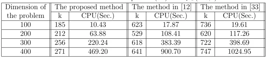
Table 1: Numerical results for problem (6.1) withei∈(1.25,2).
Dimension of The proposed method The method in [12] The method in [33] the problem k CPU(Sec.) k CPU(Sec.) k CPU(Sec.)
100 185 10.43 623 17.87 736 19.61
200 212 63.88 529 108.41 620 117.26
300 256 220.24 618 383.39 722 398.69
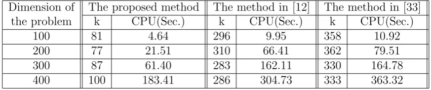
Table 2: Numerical results for problem (6.1) withei ∈(1.8,2).
Dimension of The proposed method The method in [12] The method in [33] the problem k CPU(Sec.) k CPU(Sec.) k CPU(Sec.)
100 81 4.64 296 9.95 358 10.92
200 77 21.51 310 66.41 362 79.51
300 87 61.40 283 162.11 330 164.78
400 100 183.41 286 304.73 333 363.32
Table 3: Numerical results for problem (6.1) withei∈(2,3).
Dimension of The proposed method The method in [12] The method in [33] the problem k CPU(Sec.) k CPU(Sec.) k CPU(Sec.)
100 87 4.97 303 12.23 343 13.91
200 91 23.18 339 51.53 393 55.08
300 94 60.12 321 139.94 380 154.44
400 89 136.16 335 351.83 393 391.64
Table 4: Numerical results for problem (6.1) withei∈(10,12).
Dimension of The proposed method The method in [12] The method in [33] the problem k CPU(Sec.) k CPU(Sec.) k CPU(Sec.)
100 81 4.61 196 7.06 213 7.13
200 78 19.46 304 57.93 325 59.88
300 88 57.81 356 141.58 377 149.47
400 99 168.63 389 422.36 417 480.56
Tables 1–4 show that the proposed method is more flexible and efficient for the problem tested. Moreover, it demonstrates computationally that the new method is more effective than those in [12] and [33] in the sense that the new method needs fewer iterations and less computational time.
References
[1] A. Auslender, M. Teboulle and S. Ben-Tiba,A logarithmic-quadratic proximal method for variational inequalities, Comput. Optim. Appl. 12 (1999) 31–40.
[2] A. Bnouhachem,An LQP method for pseudomonotone variational inequalities, J. Global Optim. 36 (2006) 351– 363.
[3] A. Bnouhachem, H. Benazza and M. Khalfaoui, An inexact alternating direction method for solving a class of structured variational inequalities, Appl. Math. Comput. 219 (2013) 7837–7846.
[4] A. Bnouhachem, On LQP alternating direction method for solving variational, J. Inequal. Appl. 2014 (2014):80. [5] A. Bnouhachem and M.H. Xu, An inexact LQP alternating direction method for solving a class of structured
[6] A. Bnouhachem and Q.H. Ansari,A descent LQP alternating direction method for solving variational inequality problems with separable structure, Appl. Math. Comput. 246 (2014) 519–532.
[7] A. Bnouhachem and A. Hamdi, Parallel LQP alternating direction method for solving variational inequality problems with separable structure, J. Inequal. Appl. 2014 (2014):392.
[8] A. Bnouhachem, S. Al-Homidan and Q.H. Ansari, New descent LQP alternating direction methods for solving a class of structured variational inequalities, Fixed Point Theory Appl. 2015 (2015):137.
[9] A. Bnouhachem, A. Hamdi and M.H. Xu,A new LQP alternating direction method for solving vriational inequality problems with separable structure, Optimization 65 (2016) 2251–2267.
[10] A. Bnouhachem, A. Latif and Q.H. Ansari,On the O(1/t) convergence rate of the alternating direction method with LQP regularization for solving structured variational inequality problems, J. Inequal. Appl. 2016 (2016):297. [11] A. Bnouhachem, F. Benssi and A. Hamdi, On alternating direction method for solving vriational inequality
problems with separable structure, J. Nonlinear Sci. Appl. 10 (2017) 175–185.
[12] C. Cao, D.R. Han and L.L. Xu,A new partial splitting augmented Lagrangian method for minimizing the sum of three convex functions, Appl. Math. Comput. 219 (2013) 5449–5457.
[13] G. Chen and M. Teboulle, A proximal-based decomposition method for convex minimization problems, Math. Program. 64 (1994) 81–101.
[14] J. Eckstein and D.P. Bertsekas,On the Douglas-Rachford splitting method and the proximal point algorithm for maximal monotone operators, Math. Program. 55 (1992) 293–318.
[15] J. Eckstein and M. Fukushima, Some reformulation and applications of the alternating directions method of multipliers, Large Scale Optimization: State of the Art(W. W. Hager et al, Eds.), pp. 115–134, Kluwer Acad. Publ., 1994.
[16] F. Facchinei and J.S. Pang, Finite-Dimensional Variational Inequalities and Complementarity Problems, vol. I and II. Springer Series in Operations Research. Springer, New York, 2003.
[17] M. Fortin and R. Glowinski, Augmented Lagrangian methods: Applications to the solution of boundary-valued problems, North-Holland, Amsterdam, Holland, 1983.
[18] D. Gabay and B. Mercier,A dual algorithm for the solution of nonlinear variational problems via finite-element approximations, Comput. Math. Appl. 2 (1976) 17–40.
[19] D. Gabay,Applications of the method of multipliers to variational inequalities, in Augmented Lagrange Methods: Applications to the Solution of Boundary-valued Problems, M. Fortin and R. Glowinski, Eds., NorthHolland, Amsterdam, 299–331, 1983.
[20] R. Glowinski,Numerical methods for nonlinear variational problems, Springer-Verlag, New York, 1984.
[21] R. Glowinski and P. Le Tallec, Augmented Lagrangian and operator-splitting methods in nonlinear mechanics, SIAM Studies in Applied mathematics, Philadelphia, PA, 1989.
[22] B.S He, H. Yang and S.L. Wang,Alternating directions method with self-adaptive penalty parameters for monotone variational inequalities, J. Optim. Theory Appl. 106 (2000) 349–368.
[23] B.S. He, L.Z. Liao, D.R. Han and H. Yang,A new inexact alternating directions method for monotone variational inequalities, Math. Program. 92 (2002) 103–118
[24] B.S. He and J. Zhou, A modified alternating direction method for convex minimization problems, Appl. Math. Lett. 13 (2000) 123–130.
[25] B.S. He, L.Z. Liao, D.R. Han and H. Yang,A new inexact alternating directions method for monotone variational inequalities, Math. Program. 92 (2002) 103–118
[26] B.S. He,Parallel splitting augmented Lagrangian methods for monotone structured variational inequalities, Com-put. Optim. Appl. 42 (2009) 195–212.
[27] Z.K. Jiang and A. Bnouhachem,A projection-based prediction-correction method for structured monotone varia-tional inequalities, Appl. Math. Comput. 202 (2008) 747–759.
[28] J Z.K. Jiang and X.M. Yuan, New parallel descent-like method for sloving a class of variational inequalities, J. Optim. Theory Appl. 145 (2010) 311–323.
[29] S. Kontogiorgis and R.R. Meyer,A variable-penalty alternating directions method for convex optimization, Math. Program. 83 (1998) 29–53.
[30] M. Li,A hybrid LQP-based method for structured variational inequalities, Int. J. Comput. Math. 89 (2012) 1412– 1425.
[31] B. Martinet, Regularization d’inequations variationelles par approximations sucessives, Revue Francaise d’Informatique et de Recherche Op´erationelle 4 (1970) 154–159.
[32] A. Nagurney and P. Ramanujam,Transportation network policy modeling with goal targets and generalized penalty functions, Transportation Science 30 (1996) 3–13.
problem, Comput. Math. Appl. 60 (2010) 1515–1524.
[34] R.T. Rockafellar,Augmented Lagrangians and applications of the proximal point algorithm in convex programming, Math. Oper. Res. 1 (1976) 97–116.
[35] R.T. Rockafellar,Monotone operators and the proximal point algoritm, SIAM J. Control Optim. 14 (1976) 877– 898.
[36] M. Tao M. and X.M. Yuan, On the O(1/t) convergence rate of alternating direction method with logarithmic-quadratic proximal regularization, SIAM J. Optim. 22 (2012) 1431–1448.
[37] M. Teboulle,Convergence of proximal-like algorithms, SIAM J. Optim. 7 (1997) 1069–1083.
[38] K. Wang, L.L.Xu and D.R. Han, A new parallel splitting descent method for structured variational inequalities, J. Ind. Manag. Optim. 10 (2014) 461–476.