Printed in The Islamic Republic of Iran, 2014 © Shiraz University
MULTIPLE CFO ESTIMATION IN OFDM UNDERWATER
COMMUNICATION SYSTEMS*
S. MASHDOURAND A. JAMSHIDI**
School of Electrical and Computer Engineering, Shiraz University, Shiraz, I. R. of Iran Email: [email protected]
Abstract– When channel is severely frequency selective, Orthogonal Frequency Division Multiplexing (OFDM) is a suitable candidate for high rate communications. In multipath fading channels like harsh underwater channels, due to Inter Carrier Interference (ICI) and Carrier Frequency Offset (CFO) the performance of this technique is dramatically decreased. Therefore, these effects must be alleviated to overcome the performance degradation. To do that, first the CFO’s must be estimated. In this paper, we consider an underwater channel with three sets of paths and we assume that the paths in each set have similar Doppler scale factor. For minimum transmission power, Zero Padded OFDM (ZP-OFDM) is considered. We propose a new method based on MUltiple SIgnal Classification (MUSIC) technique that facilitates the estimation of multiple CFO’s in Under Water Acoustic (UWA) channel and compare it with the derived Maximum Likelihood (ML) estimator algorithm. Simulation results show that the proposed method is robust against the received Signal to Noise Ratio (SNR) variations.
Keywords– OFDM, doppler, multiple CFO’s, MUSIC method, ML estimation
1. INTRODUCTION
The OFDM technique, a multi-carrier modulation scheme in which broadband data is transmitted in parallel as K narrowband channels on K orthogonal subcarriers, has been extensively used by the radio technology standards. It allows designing low complexity equalizers to deal with highly dispersive channels [1]. UWA channels are wideband in nature and severely suffer from time varying, multipath and frequency selectivity in its broad transmission band. Reverberation is caused mainly by the multiple reflections/diffusions/diffractions of the transmitted signal by the surface and bottom interfaces [2]. Motivated by the success of OFDM in radio channels, there is an interest in applying OFDM in underwater acoustic channels [3]-[5]. In this paper, using ZP-OFDM in the underwater acoustic channel [5] instead of CP-OFDM to minimize the transmission power it is preferred.
Time-varying channel of underwater acoustic communications due to transmitter, receiver, or surface motion induces broadband Doppler shifts that are not uniform across OFDM subcarriers. A common approach for compensating the dominant Doppler components is to estimate the time compression or dilation of packets by detecting the start of two consecutive synchronization pattern, comparing the received versus the transmitted synchronization pattern-to-pattern, and resampling the received signals to undo any compression or dilation [6]. It was shown in [7] that resampling of an OFDM signal will approximately reduce the Doppler distortion to a residual narrowband component. In fact, this residual narrowband component is the so called Doppler distortion, i.e., Carrier Frequency Offset (CFO). Note that CFO induced by the time variable channels destroys the orthogonality between OFDM subcarriers and thus degrades the system performance and increases the complexity of the equalizers [8]. Also, a UWA
channel is wide-band in nature, thus, it is more affected by CFO. This phenomenon severely reduces the performance of the OFDM system in the UWA channels [9]-[14]. To reduce the performance degradation, the effect of CFO must be compensated effectively [15].
However, for CFO compensation, first, it must be estimated. In several papers, various methods for CFO estimation have been proposed. In [4], a method based on null subcarriers energy has been suggested to estimate CFO. An iterative CFO and sparse channel estimation based on matching pursuits (MP) algorithms has been designed in [9]. In [10], adaptive algorithms of [11] are adopted for online CFO estimation. In [16], the process of removing the CFO is an iterative one, using a guess-and-check method. In the proposed method, the receiver walks through a range of possible CFO values at a step size of 0.1 Hz. At each step, it compensates the CFO before FFT processing, and then performs pilot-based channel estimation in the frequency domain. Subspace-based CFO estimators are developed to utilize the covariance matrix of the received signal with the assumption that null subcarriers are located at the end of blocks in [17] and [18]. Also, in [19] a blind ML estimator of CFO has been proposed based on two identical received blocks.
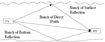
All of the previous works in this area assumed that the signal transmission paths have similar Doppler scaling factor. In this paper, we assume that the channel has three sets of paths. For each set, a different Doppler scale of other sets has been considered. In fact, the received paths in the multipath channel are divided into three sets, one of them being near to the line of sight (LOS) of the transmitter/receiver, the other is above the LOS reflected from the sea surface, and the last one lies under the LOS reflected by the bottom of the sea. As seen from Fig. 1, it is assumed that each path contains a bunch of rays with the same delay, but different from the other paths.
Fig. 1. Traveling paths between transmitter and receiver
Therefore, a different Doppler scale for each one is considered. Due to having three different Doppler scales, there will be three CFO’s in the received signal which must be estimated. In this paper, for simultaneous estimation of these three offsets, a new method is proposed based on MUltiple SIgnal Classification (MUSIC) algorithms. To comparise the proposed algorithm, we also use the Maximum Likelihood (ML) estimator and conduct some simulations based on the proposed algorithm and the ML estimator. Our proposed method and ML estimation can be applied when more Doppler scales and consequently more CFO’s are considered in the UWA channel.
The rest of this paper is organized as follows. In section 2, the UWA channel is characterized and some concepts of ZP-OFDM are described. In section 3, the MUSIC method is used to describe a CFO estimation approach. In Section 4, we present the ML method to estimate CFO’s in the received signal. In section 5, some computer simulations are conducted for the proposed MUSIC based and the ML estimation methods. Finally section 6 concludes the paper.
2. UWA CHANNEL CHARACTERIZATION AND ZP-OFDM
a) The ZP-OFDM and channel characterization
OFDM is a special case of multi-carrier transmission, where a signal data stream is transmitted over a number of lower rates subcarriers (SCs). One of the main reasons of using OFDM is to increase robustness against frequency-selective fading or narrowband interference. In OFDM, serial data are converted to parallel data in the subcarriers. If OFDM symbol duration is T, frequency space of subcarriers will be
Δf=1/T and then frequency of kth subcarrier will be fc+kΔf, where fc is the carrier frequency. By assuming
the transmitted data sample on the kth subcarrier is Sk and the number of subcarriers is N, OFDM symbol in the baseband can be written as
N k ft k j ke S t s 0 2 )
( (1) Considering (1), the transmitted signal in the pass-band is then given by
g
t f j U k ft k j
ke g t e t T T
S t x c A
( ) , 0,
Re )
( 2 2 (2) Where, Tg is the guard interval, KA is the number of active subcarriers and Kn is the number of null subcarriers. Therefore, K=KA+Kn is the total number of subcarriers. Also, g(t) does zero padding in the transmitted signal, which is described as
g T T T t T t t g , 0 , 0 1 )( (3) and UA is the active subcarriers set. ai, Cil, τil are constants over an OFDM block duration T′=T+Tg. For the channel model, we consider a multipath underwater channel that has the impulse response [5],
()
) ,
( t C t t
h l
l l
(4)
Where Cl(t) is the amplitude of lth path and τl(t) is its time delay which depends on the time t and δ is Dirac delta function. Here, three Doppler scaling factors are adopted for the paths. By considering the same scale factor for the bunch ray of each path, we can write the paths’ delays as,
t a t t a t t a
t l l l l l
l 1 1 2 2 2 3 3 3
1() , () , ()
(5)
Whereaiis Doppler scale factor of ith path, and il
is the l ray delay in the i th path. Therefore, channel impulse response can be written as follows:
l l l
l l l
l l l
t t C t t C t t C t h 3 3 2 2 1 1 ,
(6)
Using distributive law for convolution operation, the pass-band received signal can be written as,
Where L1,L2 and L3 are the number of the ray in 1st, 2nd and 3rd path sets, respectively, and n(t) is additive
noise which is zero mean and its variance has been assumed σ2. b) Compensated output and CFO representation
Various methods to Doppler scale estimation are developed in different papers. In [7], a resampling method has been proposed based on the assumption that all the paths have the same Doppler scaling factor. This is not the case in a complicated UWA channel. In this paper, we assume three paths with different scaling factor for the propagated signal. When one common Doppler scaling factor has been involved in the channel model, Doppler scaling factor can be compensated by resampling [7]. It is clear that the relation between the baseband signal~y(t)and the pass-band signal y(t)can be written as,
ytej fct
t
y() Re ~() 2 (8) The resampling method has been shown effective to compensate the scaling factor in the underwater
communications [7, 20]. This technique can be done in the pass-band or the baseband. For example, such as the work in [5], for the baseband resampling, we have
b t y t z 1 ~ ) (
~ (9)
Where,
~
y
(
t
)
is the baseband equivalent of the received signal and~
z
(
t
)
is the baseband resampled signal. To compensate the Doppler scale factors and estimate the CFO’s, we suppose that the scaling factors’ values of the different paths are close to each other. Therefore, it is possible to write ai=b+δi, δi˂˂b, this means that ai is close to b. So, a similar parameter b has been considered for all the paths. Indeed, in all paths, there is a small difference in ai’s. Here, we consider the resampling of the pass-band signaly
(
t
)
. By consideringfkfckf, separation of the summations on k and l, and using equation (4), the resampled pass-band signal z(t) can be obtained as) ( 1 1 1 1 1 1 ) ( 3 3 2 1 1 1 2 1 2 2 2 2 1 1 1 2 1 2 1 1 2 1 1 1 2 1 2 3 3 3 2 2 2 1 1 1 t t b a g e C e S e t b a g e C e S e t b a g e C e S e t z A k l c A k l c A k l c U k l l f j l t b a f k j k t b b a f j U
k l l
f j l t b a f k j k t b b a f j U
k l l
f j l t b a f k j k t b b a f j (10)
Where υ(t) is the scaled version of n(t) by factor (1+b), so, υ(t) is an additive white noise as well. By the assumptions, considering Doppler scale factor b is near to a1, a2, a3, we can use the approximation (1+ai)/(1+b)≈1. As can be seen in (7), three CFOs can be defined as follows:
c c c f b b a f b b a f b b a 1 , 1 , 1 3 3 2 2 1
1
(11)
3. MUSIC-BASED METHOD FOR CFO ESTIMATION
In this section, we use the well-known spectral estimation technique, the MUSIC algorithm, to estimate the residual CFOs. The common scale factor b can be compensated by resampling the pass-band signal, as mentioned in the previous section.
It can be seen from (10) and (11) that there are three CFO’s in the received signal that cause ICI. Some methods for CFO estimation in underwater communications are proposed based on the MUSIC method in the literature. In [5], a CFO estimation algorithm was proposed using null subcarriers for each OFDM block within a data packet. In this method, null subcarriers are used to facilitate estimation of CFO. Energy of null subcarriers is used as a cost function and CFO estimation is performed by computing minimum of the null subcarriers energy over different CFOs. In fact, the authors in [5] have proposed an exhaustive search for finding the CFO by minimizing the defined cost function. However, it seems that it is difficult to use this method for three CFO’s directly. So, in this paper, we propose a new method based on the MUSIC technique by applying an appropriate modification to this technique. For this purpose, in the next subsection we review some technical points of the MUSIC algorithm.
a) MUSIC technique
MUltiple SIgnal Classification (MUSIC) method is derived using the covariance model for the signal. In this method, it is desired to estimate the frequencies ωk , k=1,…,n, for a signal that is described by the following model:
n
k
t j ke k k t
Q
1
) (
)
( (12)
Where, Q̃(t) is defined as
n m m
t Q t
Q t Q
t)[ () ( 1) ( 1)];
( ~
Q (13)
Let the covariance matrix of (13) be
~(t)~ (t)
E
Q Q
R (14)
Where E is the expectation operation and (*) denotes the Hermitian transpose of a matrix. Now, let m
1 2 denote the eigenvalues of R arranged innon-increasing orderand let
v1,v2,,vn
be the eigenvectors associated with
1,2,,n
, respectively, and G
g1,g2,gmn
is a matrix where its columns are the set oforthogonaleigenvectors corresponding to
n1,m
.If we define
j j m
Ti e i e i
( 1)
1 )
(
a , it is shown that for each ωi, we have [11]:
) ( ) 0 ; , ,
(
i i
iGGa m n
a (15) MUSIC technique defies the inverse of the left hand side of (15) as a criterion for estimating the desired frequencies. Therefore, the locations of the peaks of the following expression will be the desired frequencies:
) ( ) (
1 )
(
a GG
a
P
(16) Sometimes (16) is called “pseudo spectrum” since it indicates the presence of sinusoidal components in
the signal, but it is not a true power spectral density. Ideally, it can be concluded from (15) that,
n m P
i i
i ( ) ( ) ;
1 )
(
a GG
In the MUSIC method, the estimation of ωi is based on (17). In practice, an estimation of matrix covariance is used in place of R, and eigenvalues and eigenvectors of this estimated covariance are used. The practical covariance matrix can be defined as,
N
i
i
i t
t
N 1
~ ~ 1
ˆ Q( )Q ( )
R
(18)
Where N is the number of samples and ti is the i th sample time. So, (17) does not hold exactly. In this case, the frequencies ωi’s can be estimated by locating the peaks of the following expression:
( )ˆˆ ( ) 1 ) ( ˆ
a G G a
P
(19) Where, Ĝis a measurement of G.
b) The proposed CFO estimation method
Now, the MUSIC method is used to estimate CFOs. If we use (19), 3kA frequencies will be estimated for expression (10), where kA is the number of active subcarriers. But, our goal is to estimate three CFOs which are added to k-dependent frequencies in each summation term in (10). So, (19) cannot be directly used to estimate CFOs. The estimation of three CFOs is performed by locating the peaks of the following expression, which is obtained by modifying the MUSIC pseudo-spectrum given in (19):
2 ) (2 2 ) ,2 ,
2 (
1
mod
i U
k
i i
ified
A
f k f
k P
a GG
a* *
(20)
Note that the MUSIC method is suitable when all frequencies are unknown and independent from each other. However, in our problem, the unknown frequencies ωi’s are not independent from each other, such that the differences between the frequencies of the subcarriers correspond to the CFOs. In the MUSIC pseudo spectrum given by (17), the denominator becomes equal to zero for each value of ωi’s. This fact can be used for finding the frequencies of subcarriers (ωi’s).Similar to this situation, the summation in the denominator of our proposed criterion in (20) becomes equal to zero when the value of ԑi is selected
as 2
2 i i
k f
. As a result, the proposed criterion (20) can be used to search the correct value of ԑi. In fact, this results in a peak for each CFO in the modified pseudo-spectrum given in (20). Therefore, the proposed method is much more compatible with our problem in this paper, because it searches only for the three CFOs. Note that this method can be used even if there are more than three Doppler scaling factors in the received signal. In the next section, we derive the ML estimate of the CFOs in our problem to compare the results of the proposed method based on the MUSIC technique.
4. ML METHOD FOR CFO ESTIMATION
In this section, for the sake of comparison with our proposed MUSIC technique, the ML method is used for simultaneous estimation of CFO’s. Using the considered assumptions in the previous sections, the received pass-band signal in (10) can be rewritten as:
t
t ge C e
S e
t g e C e
S e
t g e C e
S e
t z
k l
l f j l ft k j k t b
b a f j
k l
l f j l ft k j k t b
b a f j
k l
l f j l ft k j k t b
b a f j
k l c
k l c
k l c
3 2
3 2 1
2
2 2
2 2 1
2
1 2
1 2 1
2
3 3
2 2
1 1
The above equation is derived from (10) when (1+ai)/(1+b)s are considered equal to 1. The above received signal consists of three parts. In each part, we define:
k
Ce2 , i1,2,3 Hl
f j il
i il k
(22)
By substituting (22) in (21), the pass-band received signal can be written as
k S e
t H e e S k H e e S k H e t z k ft k j k t b b a f j k ft k j k t b b a f j k ft k j k t b b a f j c c c
2 3 1 2 2 2 1 2 2 1 1 2 3 2 1 ) ( (23)To obtain the discrete time model of z(t), we sample the received signal in (23) by sampling time Ts. Therefore, we have
s s fn
nT t t z n z
(24)
Let us define the following parameters for convenience:
i
k iiik H kS f
S~ , 2 , 2 (25) Considering these definitions and combining (24) and (25), we obtain the following for the discrete time signal model of its equivalent continuous baseband signal.
ke
n n NS e k S e k S n z k f n k j k f n k j k f n k j s s s ,..., 2 , 1 , ~ ~ ~ 3 2 1 3 2 1
(26)To write the problem in a formal structure, now, we define three matrices and three vectors as
~ 0 ~1 ~ 1
, 1,2,3 3 , 2 , 1 , 1 1 i K S S S i e e diag T i i i N jji i
i i
S
p (27)
Where N and K are the number of samples and subcarriers, respectively, and T denotes the transpose operation. Also, we know that the well-known DFT (FFT) matrix is defined as
1 1 1 ) 1 (1
1
1
1
1
K N j N j K j je
e
e
e
w
(28)Then, using (26)-(28), the vector for the received signal can be arranged as
υ ws p ws p ws p
z 1 1 2 2 3 3
Where υ is zero mean white Gaussian noise vector, and z is the received signal vector. If variance of the Gaussian noise is σ2Ι, then it is easy to show that the logarithmic likelihood function can be written as
z pws p2ws2 p3ws3z pws p2ws2 p3ws3
φ z 1 1 * 1 1 2 2 1 ln ) ; ( ln N
p (30)
Where function p(.) defines the probability density function, ‘*’ denotes the Hermitian operation and
φ=[ϕ1 ϕ2 ϕ3] is the desired vector that must be estimated. By using Newton-Raphson algorithm, φcan be
estimated iteratively as shown below:
k k k k k k k k k p p p , 3 3 , 2 2 , 1 1 3 2 1 3 2 1 1 , 3 , 2 , 1 1 , 3 1 , 2 1 , 1 ) ; ( ln ) ; ( ln ) ; ( ln , , z z zI (31)
Where I is Fisher information matrix. Here, this information matrix will be
2 3 2 2 3 2 1 3 2 3 2 2 2 2 2 1 2 2 3 1 2 2 1 2 2 1 2 3 2 1 ) ; ( ln ) ; ( ln ) ; ( ln ) ; ( ln ) ; ( ln ) ; ( ln ) ; ( ln ) ; ( ln ) ; ( ln , , z z z z z z z z z I p E p E p E p E p E p E p E p E p
E (32)
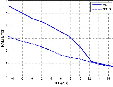
Now, we are ready to discuss the convergence of (31) and Cramer Rao Lower Bound (CRLB) to compare the performance of the MUSIC and ML methods with the ideal lower bound on the simulated Mean Square Errors (MSEs). The convergence of (31) is dependent on the number of samples, i.e., N in (26) and other parameters of the considered OFDM systems. In this paper, we consider N as high as where ML method captured the best performance in the MSE sense. Simulations show that after merely 10 iterations the MSE of the ML method reaches the minimum level for a given SNR.
We know that a useful factor which provides a lower bound on the variance of any unbiased estimator is CRLB. At least it offers a benchmark for the sake of comparison. The parameters’ vector, like the case of this paper, allows obtaining a bound on the variance of each element of the unknown vector that must be estimated. The CRLB for each element of the unknown vector is the i th element of the main diagonal in the inverse of Fisher matrix, that means
P
ii i I , ... , ) ˆ var( 1 1 θ
θ (33)
Where I(θ) is the P×P Fisher information matrix and it’s elements are defined by,
I
E p i j Pj i j
i ; , 1,...,
) ; ( ln ) ( 2 ,
xθ (34)
5. NUMERICAL RESULTS AND DISCUSSIONS
In this section, some computer simulations of CFO estimation in the UWA channels are conducted. For highlighting the MUSIC-based results, the considered values of CFOs in some of the simulations are higher than usual, moreover, the differences between the CFOs have been assumed more than typical values. Note that we have also considered some simulations with usual CFO values. In all of the simulations, the estimation of the angular frequency have been assumed, i.e., ωi’s are in the interval of (-π,
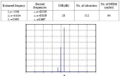
π). So, the actual and estimated values are ωi = (2πԑi/fs) and ῶi = (2πԑ̂i/fs), respectively, where fs is the sampling frequency. Through these relations one can easily compute the CFO value. For the sake of comparison, we have run the simulations for different OFDM systems. Table I shows our proposed MUSIC based method estimations. Besides, we summarize the OFDM system parameters and SNR value of our first scenario in this table. In this simulation, OFDM symbol duration is 75ms. As we can see from Table I, the estimated values and the real values are very close to each other. Figure 1 shows the pseudo-spectrum according to the contents of Table 1. This figure exhibits the results of the MUSIC-based method for the first scenario.
Table 1. Simlation results of the MUSIC based method for the first scenario
Estimated frequncy frequencies Desired SNR(dB) No. of subcarriers No. of OFDM symbols
3682 . 0 ˆ
0184 . 0 ˆ
3508 . ˆ
3 2 1
3667 . 0
0189 . 0
3516 . 0
3 2 1
20 512 64
Fig. 1. Pseudo-spectrum of MUSIC based CFO estimation for the first scenario given in Table 1
The second and third scenarios are OFDM systems with parameters given in Table 2 and 3. In these scenarios we consider that the OFDM symbol duration is 42.66ms. The simulations have been done for two different SNRs.
Table 2. Desired and estimated CFO for the second scenario with SNR=12.5dB using MUSIC based method
Estimated frequencies frequencies Desired NO. of subcarriers NO. of OFDM symbols
9001083 . 0 ˆ
8503321 . 0 ˆ
8010625 . 0 ˆ
3 2 1
95 . 0
9 . 0 85 . 0
3 2 1
512 64
Pseud
o s
pectrum
-4 -3 -2 -1 0 1 2 3 4
0 1 2 3 4 5 6 7 8
p
Table 3. Desired and estimated CFO for the second scenario with SNR=20 dB using MUSIC based method
Estimated frequencies Desired frequencies subcarriers NO. of NO. of OFDM symbols
900867 . 0 ˆ
850097 . 0 ˆ
800503 . 0 ˆ
3 2 1
9 . 0
85 . 0
8 . 0
3 2 1
512 64
The estimation results are shown in Table 2 and 3 for moderate SNR=12.5 dB and high SNR=20 dB, respectively. In Tables 4 and 5, The estimation results of the proposed MUSIC method for SNR=0 dB and SNR=15 dB are shown, respectively. The parameters of the OFDM system have also been summarized in these tables. These results show that at the low SNR, i.e., SNR=0 dB, the estimated frequencies in the proposed method are close to actual values and increasing the SNR to 15 dB makes the estimated values much better. So, we can conclude that the proposed method is robust against the SNR variations.
Table 4. Desired and estimated CFO WITH SNR=0 DB using MUSIC based estimation method
Estimated
frequencies frequencies Desired iterations NO. of subcarriers NO. of No. of OFDM symbols
90026 . 0 ˆ
85045 . 0 ˆ
80008 . 0 ˆ
3 2 1
9 . 0
85 . 0
8 . 0
3 2 1
10 512 8
Table 5. Desired and estimated CFO WITH SNR=15 DB using MUSIC based estimation method
Estimated frequencies Desired frequencies
NO.of iterations
NO. of subcarriers
No. of OFDM symbols
90003 . 0 ˆ
85007 . 0 ˆ
80000 . 0 ˆ
3 2 1
9 . 0
85 . 0
8 . 0
3 2 1
10 512 8
Fig. 2. RMS error of frequency estimation in the ML and MUSIC based methods (for2)
Fig. 3. ML frequency estimation results provided by four first iterations based on Eq. (31)
-4 -2 0 2 4 6 8 10 12 14 16
0 1 2 3 4 5
6x 10
-4
SNR(dB)
RM
S Er
ro
r
ML CRLB
Fig. 4. ML estimation and CRLB versus SNR
6. CONCLUSION
In this paper, OFDM system was considered for application in UWA channel with non-uniform Doppler shifts. The channel was considered to have three Doppler scaling factors. After compensating Doppler scale factor, a new method based on MUSIC technique has been proposed for estimating residual Doppler effects that were in the form of three carrier frequency offsets. Also, estimation has been done by use of ML method. Then, computer simulation results of ML and proposed method were shown for different scenarios with different system parameters. It seems that ML based method is more complicated. We can
-4 -2 0 2 4 6 8 10 12 14 16 0
0.2 0.4 0.6 0.8 1
x 10-3
SNR(dB)
RM
S Er
ro
r
iteration=1 iteration=2 iteration=3 iteration=4
4 6 8 10 12 14 16 18
0 0.5 1 1.5 2 2.5 3 3.5 4 4.5
5x 10
-4
SNR(dB)
R
M
S Er
ro
r
see from simulations that the ML method gives more accurate estimations of desired frequencies for 10 iterations, but this method shows more computations. These more computations are related to 3×3 fisher information matrix and its inverse and iterations. If more CFOs are required to be estimated, the fisher information matrix will be bigger and ML method will be more complicated, too. Thus, in these cases, using the proposed method is better than ML method.
REFERENCES
1. Wang, Z. & Giannakis, G. B. (2000). Wireless multicarrier communications: Where fourier meets Shannon. IEEE Signal Processing Magazine, Vol. 17, No. 3, pp. 29–48.
2. Khorshidi, S. (2014). The principal component inverse algorithm for detection in the presence of reverberation using autoregressive model. Iranian Journal of Science & Technology, Transactions of Electrical Engineering, Vol. 38, No. E1, pp. 91-97.
3. Stojanovic, M. (2006). Low complexity OFDM detector for underwater channels. in Proc. Of MTS/IEEE OCEANS conference, Boston, MA.
4. Li, B., Zhou, S., Stojanovic & Freitag, L. (2006). Pilot-tone based ZP-OFDM demodulation for an underwater acoustic channel. Proc. Of MTS/IEEE OCEANS conference, boston, MA.
5. Morozov, A. K. & Preisig, J. C. (2006). Underwater acoustic communications with multicarrier modulation. Proc. Of MTS/IEEE OCEANS conference, boston, MA, Sept. 18-21.
6. Sharif, B., Neasham, J., Hinton, O. & Adams, A. (2000). A computationally efficient Doppler compensation system for underwater acoustic communications. IEEE J. Ocean. Eng., Vol. 25, No. 1, pp. 52–61.
7. Li, B., Zhou, S., Stojanovic, M., Freitag, L. & Willet, P. (2008). Multicarrier communication over underwater acoustic channels with nonuniform Doppler shifts. IEEE Journal of Oceanic Engineeting, Vol. 33, pp. 198-209. 8. Kim, B. C. & Lu, I. T. (2000). Parameter study of OFDM underwater communications system. Proc. MTS/IEEE
OCEANS, Providence, Rhode Island.
9. Kang, T. & Iltis, R. A. (2008). Itertive carrier frequency offset and channel estimation for underwater acoustic OFDM systems. IEEE J. Select. Areas Commun., Vol. 26, No. 9, pp. 1650-1661.
10. Ma, X., Tepedelenlioglu, C., Giannakis,and, G. & Barbarossa, S. (2001). Non-data_aided carrier offset estimation for OFDM with nullsubcarriers: Identifiability, algorithms, and performance. IEEE J. Select. Areas Commun., Vol. 19, No. 12, pp. 2504-2515.
11. Barbarossa, S., Pompili, M. & Giannakis, G. B. (2001). Timing and frequency synchronization of orthogonal frequency multiple access system. Proc. Int.Conf. Communications, Vol. 6, Helsinki, Finland, pp.1674-1678. 12. Prasad, R. (2004). OFDM for wireless communications systems. Artech House Publishers.
13. Stoica, P. & Moses, R. L. (2005). Spectral analysis of signals. Prentice Hall.
14. Lyonnet, B., Siclet, C. & Brossier, J. M. (2010). Maximum likelihood estimator for doppler parameter and Cramer Rao Bound in ZP-OFDM UWA channel. ISCCSP IEEE.
15. Kay, S. M. (1993). Fundamentals of statistical signal processing. Vol. 1. Estimation Theory, Prentice Hall. 16. Mason, S., Anstett, R., Anicette, N. & Zhou, S. (2007). A broadband underwater acoustic modem
implementation using coherent OFDM. National Conference of Undergraduate Research (NCUR),California. 17. Liu, H. & Tureli, U. (1998). A high efficiency carrier estimator for OFDM communications. IEEE Commun.
Lett., Vol. 2, pp. 104-106.
18. Luise, M. & Reggiannini, R. (1996). Carrier frequency offset acquisition and tracking for OFDM system. IEEE Trans. Commun., Vol. 44, pp. 1590-1598.
19. Moose, P. H. (1994). A technique for orthogonal frequency multiplexing frequency offset correction. IEEE Trans. Commun., Vol. 42, pp. 2908-2914.
20. Beaujean, P. & LeBlanc, L. R. (2004). Adaptive array processing for high speed acoustic communication in shallow water. IEEE Journal of Oceanic Engineering, Vol. 29, No. 3, pp. 807–823.