The Thirty-Third AAAI Conference on Artificial Intelligence (AAAI-19)
Learning Object Context for Dense Captioning
Xiangyang Li,
1,2Shuqiang Jiang,
1,2Jungong Han
31Key Laboratory of Intelligent Information Processing of Chinese Academy of Sciences (CAS),
Institute of Computing Technology, CAS, Beijing, 100190, China
2University of Chinese Academy of Sciences, Beijing, 100049, China
3School of Computing and Communications, Lancaster University, United Kingdom
[email protected], [email protected], [email protected]
Abstract
Dense captioning is a challenging task which not only detects visual elements in images but also generates natural language sentences to describe them. Previous approaches do not lever-age object information in imlever-ages for this task. However, ob-jects provide valuable cues to help predict the locations of caption regions as caption regions often highly overlap with objects (i.e. caption regions are usually parts of objects or combinations of them). Meanwhile, objects also provide im-portant information for describing a target caption region as the corresponding description not only depicts its properties, but also involves its interactions with objects in the image. In this work, we propose a novel scheme with an object context encoding Long Short-Term Memory (LSTM) network to au-tomatically learn complementary object context for each cap-tion region, transferring knowledge from objects to capcap-tion regions. All contextual objects are arranged as a sequence and progressively fed into the context encoding module to obtain context features. Then both the learned object context features and region features are used to predict the bound-ing box offsets and generate the descriptions. The context learning procedure is in conjunction with the optimization of both location prediction and caption generation, thus enabling the object context encoding LSTM to capture and aggregate useful object context. Experiments on benchmark datasets demonstrate the superiority of our proposed approach over the state-of-the-art methods.
Introduction
Over the past few years, significant progress has been made in image understanding. In addition to image classification (Krizhevsky, Sutskever, and Hinton 2012; Simonyan and Zisserman 2015; Hu, Shen, and Sun 2018), object detection (Ren et al. 2015; Redmon et al. 2016; Hu et al. 2018) and im-age captioning (Karpathy and Fei-Fei 2015; Xu et al. 2015; Gu et al. 2018), some more challenging tasks such as scene graph generation (Xu et al. 2017; Li et al. 2017; Kla-wonn and Heim 2018) and visual question answering (Shih, Singh, and Hoiem 2016; Anderson et al. 2018) can be im-plemented by state-of-the-art visual understanding systems. In order to reveal more details in images and alleviate the
problem ofreporting bias(Gordon and Van Durme 2013),
dense captioning (Johnson, Karpathy, and Fei-Fei 2016;
Copyright c2019, Association for the Advancement of Artificial Intelligence (www.aaai.org). All rights reserved.
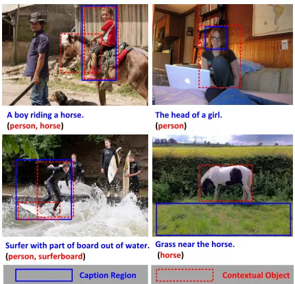
A boy riding a horse.
(person, horse)
Grass near the horse.
(horse)
The head of a girl.
(person)
Caption Region Contextual Object
Surfer with part of board out of water.
(person, surferboard)
Figure 1: Illustration of caption regions and contextual ob-jects which provide valuable cues for predicting locations and generating the target descriptions (Best viewed in color).
Yang et al. 2017) aims to describe the content of images at local region level, which not only detects visual elements but also generates natural language sentences to describe them.
Dense captioning is similar to object detection in the sense that they both need to locate regions of interest in images. The difference is that dense captioning generates natural lan-guage descriptions for regions while object detection assigns fixed class labels to them. Currently, the prevailing frame-work for dense captioning consists of three components: (i) A region proposal component is used to reduce the num-ber of candidates to be described, which is similar to the region proposal network (RPN) (Ren et al. 2015) in object detection. (ii) A language component is used to generate de-scriptions for all the proposals. (iii) A regression component is used to predict the bounding boxes of the captioned
re-gion candidates. Johnsonet al.(Johnson, Karpathy, and
0 1 2 3 4 5 6 7 8 9 1011121314
(a) the number of objects that a caption region overlap with
0 5 10 15 20 25 30 35
percentage (%)
(b) spatial relationships between caption regions and objects
0 5 10 15 20 25 30 35 40
percentage (%)
Whole Part Other contact Noncontact
Figure 2: The spatial distributions of caption regions and ob-jects in ground truth annotations on the VG-COCO dataset.
huge, Yang et al.(Yang et al. 2017) add a joint inference
module where localizing bounding boxes is jointly predicted from the features of the target regions and features of the pre-dicted descriptions. In their work, the whole image is used as context to help locate and describe caption regions.
Previous work either uses the local appearance indepen-dently or just complements it with the whole image as the context to locate and describe caption regions. In this paper, we propose a framework to exploit object context for dense captioning, transferring the knowledge from objects to cap-tion regions. Regions in dense capcap-tioning have correlacap-tions with objects from object detection mainly in two aspects.
The first one is that caption regions and objects have high overlaps in spatial locations. For example, as shown in the right of the first row in Figure 1, the region with the descrip-tion of “the head of a girl” is a part of the object instance of “person”, which is completely contained by the object. Some caption regions are almost the same with objects in locations or are the combinations of several objects. To get a holistic view, we present the statistical information of over-laps between caption regions and objects in the VG-COCO dataset (which will be elaborated in our experiments). Figure 2 (a) illustrates the number of objects that a caption region overlap with. It can be observed that most of the caption re-gions (86.5%) overlap with objects in spatial locations with the number of objects varying from 1 to 5. We categorize these caption regions according to their spatial relationships with objects into four types: (i) Caption regions which are almost the whole objects (Whole): They have Intersection-over-Union (IoU) values with objects that are bigger than 0.7, as this value is widely used to evaluate the effectiveness of a detected region in object detection (Girshick et al. 2014; Ren et al. 2015). (ii) Caption regions which are parts of ob-jects (Part): They are completely contained in obob-jects and the IoU values between them are smaller than 0.7. (iii) Cap-tion regions which have spatial contact with objects but they are neither the whole objects nor parts of objects (Other
contact). (iv) Caption regions have no spatial contact with objects (Noncontact): They are usually abstract concept
re-gions which have no overlap with any objects (i.e.sky,grass
andstreet). The examples in Figure 1 correspond to these
four kinds of relationships. Figure 2 (b) shows the percent-ages of these four kinds of regions. Objects in an image pro-vide useful indications to predict caption regions. For exam-ple, caption regions which are parts of objects appear in very distinctive locations within objects. As shown in the right of the first row of Figure 1, the caption region of a head usually tends to be near the upper middle of the person object.
The second aspect is that the descriptions for caption re-gions and objects have commonalities in semantic concepts. The descriptions for caption regions not only describe the properties such as color, shape and texture, but also involve their interactions with the surrounding objects. For example, in the first row of Figure 1, the description for the boy also involves its relationship (i.e. riding) with the horse. Even for the abstract concepts regions (i.e. Noncontact), their predic-tions are closely related with the objects in the image.
Hence, objects provide valuable cues to help locate cap-tion regions and generate descripcap-tions for them. To capture useful object information in an image, we propose a novel framework to learn complementary object context for each caption region, as shown in Figure 3. We first detect a set of objects, and then all the objects are put into a context encod-ing Long Short-Term Memory network to form informative context. The LSTM cell progressively takes each object as inputs and decides whether to retain the information from the current input or discard it, based on the information cap-tured from its previous states and current input. At last, the learned context is used as guided information to help gen-erate the descriptions and predict the bounding box offsets. The results show that the learned context is beneficial to de-scribe and locate caption regions.
In summary, our contributions are as follows: First, we propose an architecture to model complementary object con-text for dense captioning. As dense captioning and object de-tection are image understanding tasks at different levels, ex-periments demonstrate that bringing features from object de-tection can benefit dense captioning. Second, we explore dif-ferent architectures to fuse the learned context features and the features of caption regions and analyze the mechanisms for them. We also visualize the internal states of the con-text encoding LSTM cells. The visualization shows that our model can automatically select the relevant context objects to form discriminative and informative context features.
Related work
Image Captioning. Many approaches have been explored
for the task of image captioning, which aims to generate nat-ural language descriptions for the whole image. Most pre-vailing methods are based on the CNN-RNN framework.
Karpathy et al. (Karpathy and Fei-Fei 2015) use a deep
CNN to extract visual features and put these features into an RNN as the initial start word to generate image
descrip-tions. Jin et al.(Fu et al. 2017) utilize the attention
Region Features
……
Input Image
Contextual Object Features
……
ROI pooling
C
o
n
v
Conv5_3 feature map Object Detection
Region Proposal Network
Conv5_3 feature maps
Proposals Object ContextEncoding LSTM
Output
a grey shirt on a young man Young boy with one foot on a
skateboard ……
Localization and Captioning
Caption LSTM
…… ……
predictiont-1 ……
Location LSTM
Object Context
Encoding LSTM predictiont
t=N Guidance
Guidance CNN(Object1) LocSiz(Object1)
LocSiz(Object2) CNN(Object2)
LocSiz(ObjectN) CNN(ObjectN)
…… ……
+
ROI pooling
Location and Size Features CNN Features
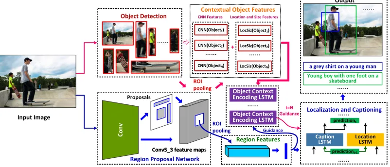
Figure 3: Overview of our framework. A region proposal network (RPN) is used to generate regions of interest (ROIs). To leverage objects information in the image, a pre-trained Faster R-CNN model is used to detect objects in the image. For both caption regions and detected objects, ROI pooling is used on top of the shared last convolutional layer (i.e. conv5 3) to get CNN features. The combination of CNN features and location and size features is used to represent each object. The features of all objects are arranged as a sequence and are put into the object context encoding LSTM with the guidance of the region features to form the complementary object context features. At last, the features of the target regions and the learned context are used to generate descriptions and bounding boxes.
each word in the sentence. Ganet al.(Gan et al. 2017)
gen-erate sentences based on detected high-level semantic con-cepts. In order to optimize captioning models on test metrics (e.g. CIDEr, SPICE), many methods based on Reinforce-ment Learning (RL) have been proposed (Rennie et al. 2017; Luo et al. 2018). In this paper, we address the task of dense captioning. For each caption region, we use the features of target regions as guidance to learn the corresponding com-plementary object context. After getting the learned context, we then use the context to guide the prediction of its descrip-tion and bounding box offset.
Object Detection.The task of object detection identifies a set of objects in the given image, providing both their pre-defined categories and the corresponding bounding box off-sets. There has been a lot of significant progress in object de-tection (Redmon et al. 2016; Liu et al. 2016; Hu et al. 2018). The first attractive work is the combination of region propos-als and CNNs (R-CNN) (Girshick et al. 2014). To achieve the goal of processing regions in an image only with a
sin-gle feedforward pass of the CNN, Girshicket al.(Girshick
2015) have modified this pipeline by sharing computation of convolutionals. Some further approaches explore region proposal strategies based on neural networks without extra algorithms to hypothesize object locations (Ren et al. 2015; Redmon et al. 2016). Our work is built on top of the region proposal network (RPN) of Faster R-CNN (Ren et al. 2015).
Similar to our work, Chenet al.(Chen and Gputa 2017)
pro-pose a Spatial Memory Network (SMN) to model object-level context to improve modern object detectors. In this work, we automatically learn complementary object context to help predict more precise locations and generate better descriptions for dense captioning.
Our Approach
The overall architecture is shown in Figure 3. In this section, we will describe each component of the proposed approach.
Region Proposal Network
We use VGG-16 (Simonyan and Zisserman 2015) as the base network. For the region proposal network, we apply
the method proposed by Renet al.(Ren et al. 2015) to
gen-erate regions of interest for dense captioning. It has 3 con-volutional layers where the first one transforms the features
of conv5 3 to suitable representations with filter size3×3.
And the remaining two layers with filter size1×1 are for
foreground/background classification and bounding box re-gression respectively. At each location, anchors with differ-ent scales and ratios are used to generate possible regions.
During training and testing, the region proposal network outputs a number of rectangular region proposals. We feed each proposal to the ROI pooling layer to obtain its fea-ture cube. Afterwards, they are flattened into a vector and pas608sed through 3 fully-connected layers. In this way, for
each generated caption regioni, we can obtain a vectorVi
of dimension D = 512 that compactly encodes its visual
appearance.
Object Context Encoding
Region Features Object Context Encoding LSTM
Vi Obj1
Object Context Encoding LSTM Obj2
Object Context Encoding LSTM ObjN
…… Guidance
Object Context Ci
t=N
bbox offset
Vi
Ci Context Decoding LSTM
prediction1 ……
predictionT-1
Caption LSTM LocationLSTM Context
Decoding LSTM
Caption LSTM LocationLSTM Context
Decoding LSTM
Caption LSTM LocationLSTM
<EOS> bbox
offset
Vi
Ci
prediction1 ……
predictionT-1
Caption
LSTM LocationLSTM Caption
LSTM LocationLSTM Caption
LSTM LocationLSTM <EOS>
Guidance
(a) (b) (c)
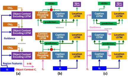
Figure 4: Illustration of object context encoding network module and region caption generation and localization mod-ule: (a) Object context encoding, (b) Object context decoded with a LSTM, and (c) Object context used as guidance.
output of the previous time step, the input of the current time step and the fixed guidance as the its current inputs. The
up-date equations at timetcan be formulated as:
it=σ(Wixxt+Wimmt−1+Wigg) (1)
ft=σ(Wf xxt+Wf mmt−1+Wf gg) (2)
ot=σ(Woxxt+Wommt−1+Wogg) (3)
ct=ftct−1+itφ(Wcxxt+Wcm+Wcgg)) (4)
mt=otφ(ct) (5)
wheregdenotes the guidance information,tranges from the
start of the input sequence to the end of it; it, ft andot
represent the input gate, forget gate, and output gate at time
stept;ctis the memory cell andmtis the hidden state;
represents the element-wise multiplication,σ(·)represents
the sigmoid function andφ(·)represents the hyperbolic
tan-gent function;W[·][·]denote the parameters of the model. In
this work, we use CNN features of the target region as the guidance for the object context encoding LSTM.
In order to obtain rich object information, we use a pre-trained Faster R-CNN to extract a set of objects from the image. Like previous approaches (Fu et al. 2017), the entire image is also utilized as a specific object region. We then put
its bounding box offset of each objectjto the ROI pooling
layer and the 3 fully-connected layers (i.e. the same architec-ture used to extract the feaarchitec-ture vectors for caption regions)
to obtain the featuresvojfrom the shared conv5 3 layer. To
acquire more information, we also extract location and size
featureslj for each objectj:
lj = [xtl W,
ytl H,
xbr
W ,
ybr H ,
jj·hj
W ·H] (6)
wherexandy are the locations of the top left and bottom
right corners of the objectj ,wj andhj are the width and
height ofj,W andHare the width and height of the image.
We then concatenate the CNN featuresvoj, the location and
size featuresljto represent objectj. At last, we use a
fully-connected layer to transform the concatenated features to the
final representationsobjjwhich has the same size withVi.
objj=Wob[voj, lj] +b (7)
where[·]denotes the concatenation operation, Wob and b
are the parameters for the fully-connected layer.
After we get the features for each detected object, we arrange them as a sequence which will be fed into the ob-ject context encoding LSTM. As the spatial information of objects is an important information for many visual tasks (Bell et al. 2016; Chen and Gputa 2017), we sort these ob-jects by their locations in the image. More accurately, they are arranged with the order of from left to right and top to down. Some other orders (e.g. area order, confidence or-der) will also be explored in our experiments. In this way,
given an image I, we utilize seq(I) to denote its object
information, which contains a sequence of representations
seq(I) ={obj1, obj2, ... , objN). For the object context de-coding procedure, we use the features of the target caption
regionvias the guidance at each step, as illustrated in Figure
4 (a). The object context encoding LSTM takes inseq(I)
progressively and encodes each object into a fixed length vector. Thus, we can obtain the encoding hidden states com-puted from:
hent =LST Men(seq(I)t, Vi, hent−1),
t= 1,2, ...N (8)
whereNis the number of objects. Once the hidden
represen-tations from all the context objects are obtained, we use the last the hidden state to represent the complementary object contextcifor the caption regioni:Ci=henN. The features
for the caption regionVi and the corresponding contextCi
will be used in the next stage to generate the description and predict the bounding box offset.
Region Caption Generation and Localization
The description for a caption region usually depicts its prop-erties and its interactions with objects in the image. So ob-ject context is of great importance for describing a caption region. It is an essential part of the input information which provides a broader understanding of the image and delivers visual cues to generate better descriptions.We explore two different architectures to leverage the
fea-tures of caption regionViand the learned object contextCi
to generate an appropriate description for each caption
re-gioni. The first architecture uses a LSTM to decode the
COCG is as follows: Because COCD has four LSTMs, it is hard to train. Removing the context decoding LSTM will alleviate the vanishing gradient problem.
For region localization, our networks are designed with the same spirits in (Yang et al. 2017). The features of the
re-gionViare put into the location LSTM as an initial word. In
the following steps, it progressively receives the outputs of the caption LSTM. After all of the predicted words (except
the token <EOS>which indicates the end of a sentence)
are put into the location LSTM, the last hidden state is used to predict the box offset. In this manner, the predicted box offset is interrelated with the corresponding description.
Training and Optimization
To obtain objects in images, we train a Faster CNN (Ren et al. 2015) model using the ResNet-101 (He et al. 2016). The model is first pre-trained on ImageNet (Russakovsky et al. 2015) dataset and then is fine-tuned on MS COCO (Lin et al. 2014) (except the test and validation images in VG-COCO). For each image, we detect 10 objects with high confidence. Because each image has an average of 7 objects (which will be introduced our experiments), most of objects will be cov-ered. For the RPN, 12 anchors are used to generate possible proposals at each location and 256 boxes are sampled for each forward procedure. The size of our vocabulary is 1000. The max length of all the sentence is set to 10. For all of the LSTM networks, the size of the hidden state is set to 512. We train the full model end-to-end in a single step of opti-mization. Our training batches consist of a single image that
has been resized so that the longer side has720pixels.
Experiments
Datasets and Evaluation Metrics
We use the Visual Genome (VG) dataset (Krishna et al. 2017) and the VG-COCO dataset which is the intersection of VG V1.2 and MS COCO (Lin et al. 2014) as the evalua-tion benchmarks.
VG.Visual Genome currently has three versions: V1.0,
V1.2 and V1.4. As the region descriptions in V1.4 are the same with the region descriptions in V1.2, we conduct our experiments on V1.0 and V1.2. The training, validation and test splits are the same with (Johnson, Karpathy, and Fei-Fei 2016). There are 77,398 images for training and 5,000 images for validation and test respectively.
VG-COCO.Even though Visual Genome provides object
annotations for each image, the target bounding boxes are much denser than the bounding boxes in other object detec-tion benchmark datasets such as MS COCO (Lin et al. 2014) and ImageNet (Russakovsky et al. 2015). For example, each image in the training set of VG V1.2 contains an average of 35.4 objects, but the average value for MS COCO is only 7.1. To get proper object bounding boxes and caption region bounding boxes for each image, the intersection of VG V1.2 and MS COCO is used in our paper, which is denoted as VG-COCO. There are 38,080 images for training, 2,489 images for validation and 2,476 for test.
For evaluation, we use mean Average Precision (mAP), which is same with (Johnson, Karpathy, and Fei-Fei 2016;
two men playing frisbee
man in red shirt
man wearing black shorts
a field of green grass
a man wearing a blue shirt
number on the shirt tall metal
pole
a pair of black shoes
the frisbee is brown
the head of a man
black shorts on man a clear
sky
a field of green grass
a tall black trash can a tree in the
background
the head of a man the head
of a man
a field of green grass
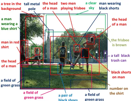
Figure 5: Illustration of detected regions and the correspond-ing descriptions generated by our method. Predictions with high confidence scores are represented.
Table 1: The results on the VG-COCO dataset (%).
Method mAP
FCLN (Johnson, Karpathy, and Fei-Fei 2016) 4.23
JIVC (Yang et al. 2017) 7.85
Max pooling 7.86
COCD 7.92
COCG 8.90
ImgG 7.81
COCG−LocSiz 8.76
COCG> 9.79
Yang et al. 2017). It measures localization and description accuracy jointly. Average precision is computed for different IoU thresholds and different Meteor scores (Lavie and Agar-wal 2007), then averaged to produce the mAP score. For lo-calization, IoU thresholds 0.3,0.4,0.5, 0.6,0.7 are used. Meanwhile, Meteor scores 0, 0.05, 0.10, 0.15,0.20,0.25 are used for language similarity. For each test image, top 300 boxes with high confidence after non-maximum suppression (NMS) with IoU of 0.7 are generated. The beam search size is set to 1 when generating descriptions. The final results are generated with a second round of NMS with IoU of 0.3.
Effectiveness of the Learned Object Context
In this section, we evaluate the effectiveness of the comple-mentary object context learned by our methods on the VG-COCO dataset. The results are shown in Table 1. We use themethod proposed by Yang et al.(Yang et al. 2017) as our
baseline method which incorporates joint inference and vi-sual context fusion (denoted as JIVC). The performance of fully convolutional localization network (denoted as FCLN)
proposed by Johnson et al.(Johnson, Karpathy, and Fei-Fei
2016) is also provided. The mAP scores for different vari-ants of models are shown in Table 1.
from 0.07 to 1.05. Several conclusions can be obtained: (i) The learned object context is effective, demonstrating its complementarity to the caption region features and its su-periority to the whole image context. For the architecture where the learned context is decoded with a LSTM (COCD), it surpasses the baseline with an improvement of 0.07. It demonstrates that the learned context is better than using the whole image as the context. While the method using max pooling to obtain the context (Max pooling) almost gets the same performance with the baseline, this demonstrates that it is better to use the proposed method to model the con-text. (ii) The architecture which uses the learned context as guidance (COCG) gets the best performance. COCG injects the context into the caption LSTM and location LSTM as guidance. Meanwhile, the context learning procedure is bun-dled together with location prediction and caption genera-tion. In this way, the context encoding LSTM is adapted to the caption and location LSTMs, and thus captures and ag-gregates useful context. (iii) The improvements of COCG mainly come from the learned region specific context. The architecture which uses the whole image as contextual infor-mation for COCG (ImgG) almost has the same performance with JIVC. Because the whole image context is fixed for each caption region, using the whole image context as the guidance is not superior to decoding it with an extra LSTM (as JIVC is a litter better than ImgG). The results demon-strate that the improvements of COCG mainly come from the learned region specific context instead of the utilization of gLSTM. (iv) The results show that only using the CNN
features to represent objects (COCG−LocSiz) leads a little
drop in the performance. The experiments also show that learning the complementary object context on the ground truth objects (COCG>) can obtain better performance. It demonstrates that accurate object bounding boxes are bene-ficial to obtain better results.
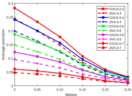
Figure 5 shows some examples generated by our method which automatically learns complementary object context for each caption region. Figure 6 shows quantitative compar-ison between the baseline (JIVC) and our method (COCG). With the Meteor score of 0, our proposed method obtains promising improvements. The results show that our method can obtain better locations. Meanwhile, it is illustrated that the proposed method obtains better performance at all set-tings, demonstrating that our complementary object context is useful for both describing and locating caption regions. Figure 7 shows several examples which qualitatively demon-strate that our method is better both at generating descrip-tions and predicting bounding box offsets. The last column in Figure 7 shows a negative example, as the generated cap-tion of COCG is slightly worse than the one of JIVC.
Context Encoding with Different Orders
For the evaluations above, we only use the location order to arrange the detected objects. In this section, we evalu-ate the performance when the objects are sorted with dif-ferent orders. Besides location order which has been used, we explore the other two kinds of orders: area and confi-dence. Area order is that context objects are sorted by their areas from big to small, as we often focus on big objects
0 0.05 0.10 0.15 0.20 0.25
Meteor
0 0.05 0.1 0.15 0.2 0.25 0.3
Average precision
COCG-0.3 JIVC-0.3 COCG-0.4 JIVC-0.4 COCG-0.5 JIVC-0.5 COCG-0.6 JIVC-0.6 COCG-0.7 JIVC-0.7
Figure 6: Average precision with different Meteor scores and different IoU thresholds on the VG-COCO dataset.
Table 2: The mAP performance on the VG-COCO dataset when context objects are arranged with different orders (%).
Method mAP
Location 8.90
Area 8.74
Confidence 8.89
and neglect small objects. Confidence order is that context objects are sorted with their confidence scores from big to small, where the confidence scores are provided by the ob-ject detection model. Table 2 shows the mAP for different orders. It can be observed that location order achieves the best performance and the other two also obtain comparable performance. So in the following sections, we only use the location order to arrange the objects.
Results on Visual Genome
We also evaluate the effectiveness of our method on Visual Genome (VG) dataset. The results are shown in Table 3. Leveraging the object context in the image, we achieve state-of-the-art performance. The proposed method obtains a rela-tive gain of 5.5% on VG V1.0 and a relarela-tive gain of 4.3% on VG V1.2. The gains are smaller than the gain in VG-COCO. The reasons are follows: First, the object detection model is only trained on MS COCO thus it have no knowledge about objects information in VG. Second, for each image, we only detect 9 images. We have not experimented with the num-ber of objects, it is possible that the improved recall from additional objects may improve the performance.
Visualized Results
As the gates of the LSTM architecture (whose activations
range from0 to1) store read, write and reset information
horse grazing on grass
horse is eating grass
(IoU: 0.80, Meteor: 0.24)
horse is white
(IoU: 0.79, Meteor: 0.13)
white shoe on a foot
white shoe on the women
(IoU: 0.68, Meteor: 0.33)
shoe on the woman
(IoU: 0.63, Meteor: 0.18)
a baseball hat the guy is wearing
a man is wearing a white hat
(IoU: 0.75, Meteor: 0.19)
a man with hat
(IoU: 0.72, Meteor: 0.11)
thin clouds in the sky
a light blue sky
(IoU: 0.50, Meteor: 0.12)
the white sky
(IoU: 0.70, Meteor: 0.13)
Figure 7: Qualitative comparisons between baseline (JIVC) and our method (COCG). The green box, the red box and the blue box are the grounding truth, the prediction of JIVC and the prediction of COCG respectively (Best viewed in color).
Table 3: The mAP performance on V1.0 and V 1.2 (%).∗
indicates that the results are obtained by our implementation.
Method VG V1.0 VG V1.2
FCLN (Johnson et al. 2016) 5.39
-FCLN∗(Johnson et al. 2016) 5.02 5.16
JIVC (Yang et al. 2017) 9.31 9.96
JIVC∗(Yang et al. 2017) 9.28 9.73
ImgG 9.25 9.68
COCD 9.36 9.75
COCG 9.82 10.39
object context encoding LSTM retains valuable context in-formation and attenuates unimportant inin-formation. Figure 8 shows two examples from the test set of VG-COCO. For the example in the first row of Figure 8, to obtain the comple-mentary object context for the region which is described as “a man wearing shorts”, the LSTM selects and propagates the most relevant object which is labeled as 5 (an object in-stance of person), as the mean input gate activations for this object is bigger than others. While for the example in the second row, the LSTM has big input gate activations for the object which is labeled as 6. The visualization indicates that meaningful patterns can be learned by the context encoding LSTM. By automatically selecting and attenuating context objects, the context encoding LSTM can generate rich com-plementary object context for each caption region.
Conclusion
In this work, we have demonstrated the importance of learn-ing object context for dense captionlearn-ing, as caption regions and objects not only have a high degree of overlap in their spatial locations but also have a lot of commonalities in their semantic concepts. To transfer knowledge from detected ob-jects to caption regions, we introduce a framework with an object context encoding LSTM module to explicitly learn complementary object context for locating and describing each caption region. The object context encoding LSTM progressively receives features from context objects to
cap-2
3 4
5 6
7 8
9
10
2
3 4
5 6
7 8
9
10
a man wearing shorts
a blue and white umbrella
1
1
Figure 8: The visualization of the object context encod-ing LSTM. The first column shows the images, where blue boxes are the detected objects, the red box is the target cap-tion region and the text is the generated descripcap-tion. The top of the second column shows the mean input gate activations for each object and the bottom shows the min-max normal-ization of them. Because the hidden state size of the object context encoding LSTM is 512, the gate activations are 512 dimensional vectors (Best viewed in color).
ture and aggregate rich object context features. After getting the learned complementary object context features, the con-text features and the region features are effectively combined to predict descriptions and locations. We explore the capa-bilities of different architectures and achieve promising re-sults on benchmark datasets. In future work, we will exploit high-level semantic information from objects to obtain more useful cues for locating and describing caption regions.
Acknowledgements
by National Program for Special Support of Eminent Pro-fessionals and National Program for Support of Top-notch Young Professionals.
References
Anderson, P.; He, X.; Buehler, C.; Teney, D.; Johnson, M.; Gould, S.; and Zhang, L. 2018. Bottom-up and top-down at-tention for image captioning and visual question answering.
InCVPR, 6077–6086.
Bell, S.; Zitnick, C. L.; Bala, K.; and Girshick, R. 2016. Inside-Outside Net: Detecting objects in context with skip
pooling and recurrent neural networks. In CVPR, 2874–
2883.
Chen, X., and Gputa, A. 2017. Spatial memory for context
reasoning in object detection. InICCV, 4106–4116.
Fu, K.; Jin, J.; Cui, R.; Sha, F.; and Zhang, C. 2017. Align-ing where to see and what to tell: image captionAlign-ing with
region-based attention and scene-specific contexts. IEEE
Transactions on Pattern Analysis and Machine Intelligence 39(12):2321–2334.
Gan, Z.; Gan, C.; He, X.; Pu, Y.; Tran, K.; Gao, J.; Carin, L.; and Deng, L. 2017. Semantic compositional networks for
visual captioning. InCVPR, 2630–2639.
Girshick, R.; Donahue, J.; Darrell, T.; and Malik, J. 2014. Rich feature hierarchies for accurate object detection and
segmentation. InCVPR, 580–587.
Girshick, R. 2015. Fast R-CNN. InICCV, 1440–1448.
Gordon, J., and Van Durme, B. 2013. Reporting bias and
knowledge acquisition. InAutomated knowledge base
con-struction Workshop, 25–30.
Gu, J.; Cai, J.; Wang, G.; and Chen, T. 2018.
Stack-captioning: Coarse-to-fine learning for image captioning. In
AAAI, 6837–6844.
He, K.; Zhang, X.; Ren, S.; and Sun, J. 2016. Deep residual
learning for image recognition. InCVPR, 770–778.
Hu, H.; Gu, J.; Zhang, Z.; Dai, J.; and Wei, Y. 2018. Relation
networks for object detection. InCVPR, 3588–3597.
Hu, J.; Shen, L.; and Sun, G. 2018. Squeeze-and-excitation
networks. InCVPR, 7132–7141.
Jia, X.; Gavves, E.; Fernando, B.; and Tuytelaars, T. 2015. Guiding Long-Short Term Memory for image caption
gena-ration. InICCV, 2407–2415.
Johnson, J.; Karpathy, A.; and Fei-Fei, L. 2016. Densecap: Fully convolutional localization networks for dense
caption-ing. InCVPR, 4565–4574.
Karpathy, A., and Fei-Fei, L. 2015. Deep visual-semantic
alignments for generating image descriptions. In CVPR,
3128–3137.
Klawonn, M., and Heim, E. 2018. Generating triples with
adversarial networks for scene graph construction. InAAAI,
6992–6999.
Krishna, R.; Zhu, Y.; Groth, O.; Johnson, J.; Hata, K.; Kravitz, J.; Chen, S.; Kalantidis, Y.; Li, L.-J.; Shamma, D. A.; Bernstein, M.; and Fei-Fei, L. 2017. Visual Genome: Connecting language and vision using crowdsourced dense
image annotations. International Journal of Computer
Vi-sion123(1):32–73.
Krizhevsky, A.; Sutskever, I.; and Hinton, G. E. 2012.
Imagenet classification with deep convolutional neural
net-works. InNIPS, 1097–1105.
Lavie, A., and Agarwal, A. 2007. METEOR: An automatic metric for MT evaluation with high levels of correlation with
human judgments. InACL, 228–231.
Li, Y.; Ouyang, W.; Zhou, B.; Wang, K.; and Wang, X. 2017. Scene graph generation from objects, phrases and region
captions. InICCV, 1270–1279.
Lin, T.-Y.; Maire, M.; Belongie, S.; Bourdev, L.; Girshick, R.; Hays, J.; Perona, P.; Ramanan, D.; Zitnick, C. L.; and Doll´ar, P. 2014. Microsoft COCO: Common object in
con-text. InECCV, 740–755.
Liu, W.; Anguelov, D.; Erhan, D.; Szegedy, C.; Reed, S.; Fu, C.-Y.; and Berg, A. C. 2016. SSD: Single shot multibox
detector. InECCV, 21–37.
Luo, R.; Price, B.; Cohen, S.; and Shakhnarovich, G. 2018. Discriminability objective for training descriptive captions.
InCVPR, 6964–6974.
Palangi, H.; Deng, L.; Shen, Y.; Gao, J.; He, X.; Chen, J.; Song, X.; and Ward, R. 2016. Deep sentence embedding using long short-term memory networks: Analysis and
ap-plication to information retrieval. IEEE/ACM Trans. Audio,
Speech, Languag. Proces.24(4):694 – 707.
Redmon, J.; Divvala, S.; Girshick, R.; and Farhadi, A. 2016. You only look once: Unified, real-time object detection. In
CVPR, 779–788.
Ren, S.; He, K.; Girshick, R.; and Sun, J. 2015. Faster R-CNN: Towards real-time object detection with region
pro-posal networks. InNIPS, 91–99.
Rennie, S. J.; Marcheret, E.; Mroueh, Y.; Ross, J.; and Goel, V. 2017. Self-critical sequence training for image
caption-ing. InCVPR, 1179–1195.
Russakovsky, O.; Deng, J.; Su, H.; Krause, J.; Satheesh, S.; Ma, S.; Huang, Z.; Karpathy, A.; Khosla, A.; Bernstein, M.; Berg, A. C.; and Fei-Fei, L. 2015. Imagenet large scale
visual recognition challenge.International Journal of
Com-puter Vision115(3):211 – 252.
Shih, K. J.; Singh, S.; and Hoiem, D. 2016. Where to
look: Focus regions for visual question answering. InCVPR,
4613–4621.
Simonyan, K., and Zisserman, A. 2015. Very deep
convolu-tional networks for large-scale image recognition. InICLR.
Xu, K.; Ba, J.; Kiros, R.; Cho, K.; Courville, A.; Salakhutdi-nov, R.; Zemel, R.; and Bengio, Y. 2015. Show, attend and tell: Neural image caption generation with visual attention.
InICML, 2048–2057.
Xu, D.; Zhu, Y.; Choy, C. B.; and Fei-Fei, L. 2017. Scene
graph generation by iterative message passing. In CVPR,
3097–3106.
Yang, L.; Tang, K.; Yang, J.; and Li, L.-J. 2017. Dense
captioning with joint inference and visual context. InCVPR,