University of Mazandaran, Iran
http://cjms.journals.umz.ac.ir
ISSN: 1735-0611
CJMS.3(1)(2014), 25-37
Numerical solution of nonlinear Hammerstein integral equations through Legendre-Bernstein basis
Farshid Mirzaee 1 and Sasan Fathi
1 Department of Mathematics, Faculty of Science, Malayer University, Malayer, 65719-95863, Iran
Abstract. In this study a numerical method is developed to solve the Hammerstein integral equations. To this end, the kernel has been approximated using the least-squares approximation schemes based on Legendre-Bernstein basis. The Legendre polynomials are orthogonal and this property improves the accuracy of the approx-imations. Also the nonlinear unknown function has been approxi-mated by using the Bernstein basis. The useful properties of Bern-stein polynomials help us to transform HammerBern-stein integral equa-tion to solve a system of nonlinear algebraic equaequa-tions.
Keywords: Nonlinear Hammerstein integral equations, Bernstein basis, Legendre basis, Orthogonal polynomials.
2000 Mathematics subject classification: 45B05, 45D05, 45G10, 65D30.
1. Introduction
The Bernstein form of a polynomial offers valuable insight into its geo-metrical behavior, and has thus won widespread acceptance as the basis for B´ezier curves and surfaces. For least-squares approximation prob-lems, on the other hand, the use of orthogonal bases, such as the Le-gendre polynomials [3,5,7], permits simple and efficient constructions for convergent sequences of approximates.
1Corresponding author: [email protected], [email protected]
Received: 25 Feb 2012 Revised: 25 May 2013 Accepted: 29 May 2013
In this paper, we consider the nonlinear Fredholm-Hammerstein inte-gral equations and nonlinear Volterra-Hammerstein inteinte-gral equations respectively by the general forms [1,8],
g(s) = f(s) +λ
∫ 1
0
k(s, t)F(t, g(t))dt, (1.1)
g(s) = f(s) +λ
∫ s
0
k(s, t)F(t, g(t))dt ; 0≤s≤1, (1.2)
where the parameterλand functionsf(s), k(s, t) andF(s, t) are known and g(s) is unknown function. It is also assumed that all of these func-tions areL2-Functions on [0,1], and g(s)∈C[0,1].
In the following we will introduce the Legendre and Bernstein poly-nomials and some properties of them used in this article.
1.1. Legendre polynomials. To emphasize symmetry properties of Legendre polynomials, they are traditionally defined on the interval [−1,+1], but for our purposes it is preferable to map this to [0,1]. The Legendre polynomialsLk(u) onu∈[0,1], can be generated through the recurrence relation [4],
(k+1)Lk+1(u) = (2k+1)(2u−1)Lk(u)kLk1(u) ; k= 1,2,· · · , (1.3)
commencing with L0(u) = 1 andL1(u) = 2u−1. This gives, in the first few instances
L0(u) = 1,
L1(u) = 2u−1,
L2(u) = 6u2−6u+ 1,
L3(u) = 20u3−30u2+ 12u−1, ..
.
The orthogonality of these polynomials is expressed by the relation ∫ 1
0
Lj(u)Lk(u)du=
{ 1
2k+1 j=k 0 j̸=k .
Now for arbitrary function f(u) on [0,1], we can express it in the Le-gendre form,
f(u)≃PN(u) = N
∑
j=0
where the coefficients lj, for Legendre polynomials are obtained from following relation
lk= (2k+ 1)
∫ 1
0
Lk(u)f(u)du ; k= 0,1,· · ·, N. (1.5)
1.2. Bernstein polynomials. (N+1)-Bernstein basic function on [0,1], are defined by using the following relation [2],
Bi,N(u) =
(
N i
)
ui(1−u)N−i ; i= 0,1,· · · , N. (1.6)
In the follow, some properties of Bernstein polynomials have been ex-pressed and used in this article,
• The product of a power basic function and a Bernstein basic function,
umBi,N(u) =
(N
i
) (N+m
i+m
)Bi+m,N+m(u). (1.7)
• The product of two Bernstein basic functions,
Bi,j(u)Bk,m(u) =
(j
i
)(m
k
) (j+m
i+k
)Bi+k,j+m(u). (1.8)
• The expression of power basic functions in the Bernstein form and vice versa,
Bk,N(u) = N
∑
i=k
(−1)i−k (
N i
)(
i k
)
ui. (1.9)
LetBst= [B0,N(s), B1,N(s),· · · , BN,N(s)] andSt= [1, s, s2,· · ·, sN] then
Bs=M S and S=M−1Bs, (1.10) where
M =
(−1)0(N0)(00) (−1)1(N1)(10) · · · (−1)N(NN)(N0) 0 (−1)0(N1)(11) · · · (−1)N−1(NN)(N1)
..
. . .. . .. ...
0 · · · 0 (−1)0(NN)(NN)
(1.11)
• All the basic functions have the same definite integral over [0,1], namely
∫ 1
0
Bi,N(u)du= 1
• The produced matrix from the integration over the product of two bases in form T =∫01BsBstds,
whereT is a (N+1)×(N+1) matrix by elements in the following form
Ti+1,j+1 = (N
i
)(N
j
)
(2N + 1)(i2+Nj) ; i, j= 0,1,· · ·, N. (1.13)
• Operational matrix of integration
LetBtt= [B0,N(t), B1,N(t),· · · , BN,N(t)], andτt= [1, t, t2,· · · , tN], then the integration of vector Bt is given by
∫ s
0
Btdt≃P Bs, (1.14)
wherePis the (N+1)×(N+1) operational matrix for integration and is given in [10]. By using of (1.11), we have
∫ s
0
Btdt=
∫ s
0
M τ dt=M
∫ s
0
τ dt=M
s
1 2s
2 .. . 1 N+1sN+1
=M MpSp,
(1.15) where Spt= [s, s2,· · · , sN+1], andMp is the following matrix
Mp =
1 0 0 · · · 0 0 12 0 · · · 0 0 0 . .. ... ... ..
. ... . .. ... 0 0 0 · · · 0 N1+1
(N+1)×(N+1)
, (1.16)
According to (1.11), we had S = M−1Bs. Therefore for k = 0,1,· · · , N, we have
sk=M[−k+1]1 Bs, (1.17)
both sides of it at Bs and integration on [0,1], we have
CN+1=T−1
∫ 1
0
sN+1Bsds=T−1 ∫1 0 s
N+1B 0,N(s)ds ∫1
0 s
N+1B 1,N(s)ds
. . .
∫1 0 s
N+1B
N,N(s)ds =
T−1
2N+ 2
(N 0 ) (2N+1
N+1
) (N
1
) (2N+1
N+2 ) . . . (N N ) (2N+1
2N+1
) . (1.18) now assume B =
M[2]−1 M[3]−1
.. .
M[−N1+1] CNt+1
, (1.19)
then Sp ≃ BBs. Therefore we have the operational matrix of integration P =M MpB.
1.3. The expression of the Legendre polynomials in the Bern-stein form. In this scale, we expand a favorite polynomial such as
PN(s) in terms of Legendre-Bernstein basis. That is, we combine two bases Legendre and Bernstein, and then calculate expansion coefficients. The Legendre polynomialsLk(s) can be expressed in the Bernstein basis
Bs of degree N as
Lk(s) = N
∑
j=0
Λk,jBj,N(s) ; k= 0,1,· · · , N, (1.20)
where [4],
Λk,j = 1 (N
j
)
min∑(j,k)
i=max(0,j+k−N)
(−1)k+i ( k i )( k i )(
N −k j−i
)
; j, k= 0,1,· · · , N.
(1.21) Now considering the polynomial PN(s) of degree N, as expressed in (1.4), we can transform it in the Bernstein form as
PN(s) = N
∑
k=0
lkLk(s) = N
∑
k=0
lk
∑N
j=0
Λk,jBj,N(s)
=
N
∑
j=0
bjBj,N(s),
where
bj = N
∑
k=0
Thatbjare expansion coefficients ofPN(s), in terms of Legendre-Bernstein basis. Similarly, we can calculate expansion coefficients of least squares approximation of kernelk(s, t), based on Legendre-Bernstein basis. Let
Lts= [L0(s), L1(s),· · ·, LN(s)], then fork(s, t) we have
k(s, t) = LtsKLt
= N
∑
m=0 N
∑
n=0
Lm(s)km,nLn(t)
= N
∑
m=0 N
∑
n=0 ( N
∑
i=0
Λm,iBi,N(s)
)
km,n
∑N
j=0
Λn,jBj,N(t)
= N
∑
i=0 N
∑
j=0
Bi,N(s)
( N ∑
m=0 N
∑
n=0
Λm,ikm,nΛn,j
)
Bj,N(t),
where
km,n = ⟨⟨
k(s, t), Ln(t)⟩, Lm(s)⟩
⟨Ln(t), Ln(t)⟩ ⟨Lm(s), Lm(s)⟩
= (2n+ 1)(2m+ 1) ∫ 1
0 ∫ 1
0
Lm(s)Ln(t)k(s, t)dtds
= (2n+ 1)(2m+ 1) N
∑
i=0 N
∑
j=0
Λm,iΛn,j
∫ 1
0 ∫ 1
0
Bi,N(s)Bj,N(t)k(s, t)dtds
; i, j= 0,1,· · ·, N.
Let
Ci,j = N
∑
m=0 N
∑
n=0
Λm,ikm,nΛn,j ; i, j= 0,1,· · ·, N, (1.22)
or
C= ΛtKΛ. (1.23)
Then
k(s, t) = N
∑
i=0 N
∑
j=0
Bi,N(s)Ci,jBj,N(t) =BstCBt. (1.24)
2. Approximation of integral equations
Consider the equation (1.1), as follows
g(s) =f(s) +λ
∫ 1
0
setw(s) =F(s, g(s)), then we have
w(s) =F
(
s, f(s) +λ
∫ 1
0
k(s, t)w(t)dt
)
,
now if we approximate w(s), by Bernstein basis as w(s) =BstA, where
At = [a0, a1,· · ·, aN], and by using of relations (1.13),(1.24), we can write
BtsA = F
(
s, f(s) +λ
∫ 1
0
BtsCBtBttAdt
)
= F
(
s, f(s) +λBstC
(∫ 1
0
BtBttdt
)
A
)
= F(s, f(s) +λBstCT A). (2.2)
So by putting the nodes {si = Ni | i= 0,1,· · · , N} in (2.2), we get a system of nonlinear algebraic equations of (N+ 1)×(N+ 1) degree, with unknown coefficients {ai |i= 0,1,· · ·N}.
After solving this nonlinear system by using of Newton method and by software Matlab, we can approximate the solution of equation (2.1), as follows
g(s) =f(s) +λBstCT A. (2.3)
3. Apprximation of Volterra integral equations
Consider the equation (1.2), as follows
g(s) =f(s) +λ
∫ s
0
k(s, t)F(t, g(t))dt ; 0≤s≤1, (3.1)
such as Fredholm kind that we set w(s) =F(s, g(s)) then
w(s) =F
(
s, f(s) +λ
∫ s
0
k(s, t)w(t)dt
)
.
Now if we approximatew(s), by Bernstein basis as w(s) =BtsA, that
At= [a0, a1,· · ·, aN], and by using of (1.24), we can write
BstA = F
(
s, f(s) +λ
∫ s
0
BstCBtBttAdt
)
= F
(
s, f(s) +λBstC
(∫ s
0
BtBttAdt
))
Now it’s only necessary to express the integration∫0sBtBttAdtin Bern-stein basis form. By using of equation (1.11), we have
∫ s
0
BtBttAdt =
∫ s 0 M τ ( N ∑ k=0
akBk,N(t)
) dt = M ∫ s 0 ∑N
k=0akBk,N(t)
∑N
k=0aktBk,N(t) ..
. ∑N
k=0aktNBk,N(t)
dt. (3.3)
Now, we approximate all functions tjBk,N(t) in terms ofBt. Namely
tjBk,N(t)≃Bttej,k ; j, k= 0,1,· · ·, N, (3.4)
whereej,k, is a approximation coefficients vector as follows
ej,k =
ej,k0 ej,k1
.. .
ej,kN
. (3.5)
By multiplyingBt, in both sides of (3.4), and integration of them, and by using of (1.13), we have
ej,k = T−1
∫ 1
0
tjBk,N(t)Btdt
= T−1
∫1 0 t jB
k,N(t)B0,N(t)dt
∫1 0 t
jB
k,N(t)B1,N(t)dt ..
. ∫1
0 tjBk,N(t)BN,N(t)dt =
T−1(Nk)
2N+j+ 1 (N 0)
(2N+j k+j)
(N
1)
(2N+j k+j+1)
.. . (N N)
(2N+j k+j+N)
. Therefore N ∑ k=0
aktjBk,N(t) ≃ N ∑
k=0
akBttej,k= N ∑ k=0 ak (N ∑ i=0
ej,ki Bi,N(t) )
=
N ∑
i=0
Bi,N(t) ( N
∑
k=0
akej,ki ) = ∑N k=0akej,k0
∑N k=0akej,k1
. . .
∑N k=0akej,kN
Bt=A
t et j,0 et j,1 . . . et j,N Bt=A
tE j+1Bt,
0,1,· · ·, N. So
N
∑
k=0
aktjBk,N(t)≃E[j+1Bt ; j= 0,1,· · ·, N. (3.6)
Now by substituting (3.6), into (3.3), we have
BstA=F
s, f(s) +λB
t sCM
∫ s
0
c
E1Bt
c
E2Bt .. .
\
EN+1Bt
dt
. (3.7)
If we define matrix Gas follows
G=
c
E1 c
E2 .. .
\
EN+1
, (3.8)
that G is a (N + 1)×(N + 1) matrix that, it has vectorsE[j+1, j = 0,1,· · ·, N, for each row. Therefore we can write the equation (3.1), as
BstA = F
(
s, f(s) +λBstCM
∫ s
0
GBtdt
)
= F
(
s, f(s) +λBstCM G
∫ s
0
Btdt
)
,
by using of (1.13), we have
BstA=F(s, f(s) +λBstCM GP Bs
)
. (3.9)
So by putting nodes {si = Ni | i = 0,1,· · · , N} in (3.9), we get a system of nonlinear algebraic equations of (N + 1)×(N + 1) degree, with unknown coefficients{ai|i= 0,1,· · ·N}.
After solving this nonlinear system by using of Newton method and by software Matlab, we can approximate the solution of equation (3.1), as follows
g(s) =f(s) +λBstCM GP Bs. (3.10)
Assume PN(x) be an approximation polynomial of function f(x) then we have the following theorem.
Theorem 3.1. (T. Popoviciu [11]). If f(x) is continuous and ω(δ) the
modulus of continuity of f(x), then
|f(x)−PN(x)| ≤ 5 4ω(N
−1
2). (3.11)
Now we find error bound for nonlinear Volterra-Hammerstein integral equations and so, for Fredholm kind is as the same. AssumePN(s) and
g(s) be approximate and exact solutions of the integral equation (3.1), respectively, so
PN(s)−λ
∫ s
0
k(s, t)F(t, PN(t))dt=f(s) +RN(s), (3.12)
whereRN(s) is the perturbation function that depends only onPN(s). LetM ≡sup0≤s,t≤1|k(s, t)|<∞, and suppose F(t, s) satisfied in Lips-chitz condition such that
|F(t, s1)−F(t, s2)| ≤L|s1−s2|. (3.13) Let E(s) = |g(s)−PN(s)| be the error function of this method. By subtracting equation (3.12), from equation (3.1), we have
|RN(s)| ≤E(s) +|λ|M LE(s) = (1 +|λ|M L)E(s), (3.14) where by substituting (3.11), into (3.14), we obtain an error bound for the perturbation functionRN(s) such as
|RN(s)| ≤(1 +|λ|M L) 5 4ω(N
−1
2). (3.15)
4. Illustrations
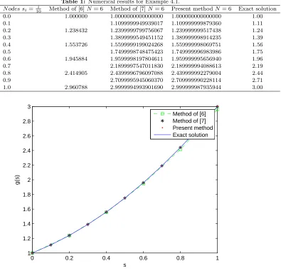
Example 4.1. Consider nonlinear Fredholm integral equation [11,12]:
g(s) = 1 +s+ (
1−3
2ln (3) +
√
3 6 π
)
s2+ ∫ 1
0
2s2tln (g(t))dt, (4.1)
Table 1: Numerical results for Example 4.1.
N odes si= 10i Method of [6]N= 6 Method of [7]N= 6 Present methodN= 6 Exact solution
0.0 1.000000 1.0000000000000000 1.000000000000000 1.00 0.1 1.1099999949939017 1.109999999879360 1.11 0.2 1.238432 1.2399999799756067 1.239999999517438 1.24 0.3 1.3899999549451152 1.389999998914235 1.39 0.4 1.553726 1.5599999199024268 1.559999998069751 1.56 0.5 1.7499998748475423 1.749999996983986 1.75 0.6 1.945884 1.9599998197804611 1.959999995656940 1.96 0.7 2.1899997547011830 2.189999994088613 2.19 0.8 2.414905 2.4399996796097088 2.439999992279004 2.44 0.9 2.7099995945060370 2.709999990228114 2.71 1.0 2.960788 2.9999994993901690 2.999999987935944 3.00
0 0.2 0.4 0.6 0.8 1
1 1.2 1.4 1.6 1.8 2 2.2 2.4 2.6 2.8 3
s
g(s)
Method of [6] Method of [7] Present method Exact solution
Figure 1. Numerical results for Example 4.1.
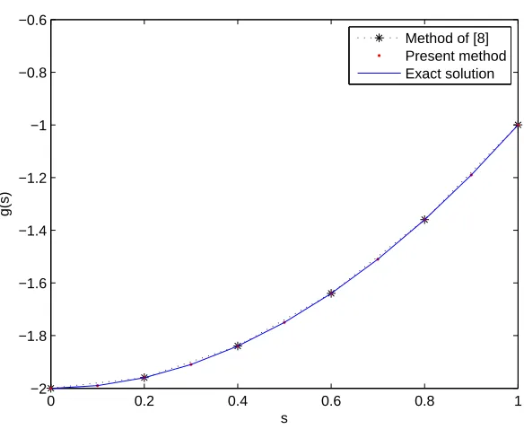
Example 4.2. Consider nonlinear Volterra integral equation [9]:
g(s) =s2−2−1 2se
(s2−2)
+1 2se
(−2)+ ∫ s
0
steg(t)dt, (4.2)
Table 2: Numerical results for Example 4.2.
N odes si=10i Method of [8] (m= 1, n= 5) Present methodN= 6 Exact solution
0.0 −1.999721 −2.000000000000000 −2.00 0.1 −1.990000220506790 −1.99 0.2 −1.959387 −1.959999536138756 −1.96 0.3 −1.909999888083469 −1.91 0.4 −1.839465 −1.840000917327985 −1.84 0.5 −1.750000310331762 −1.75 0.6 −1.639457 −1.639998696711833 −1.64 0.7 −1.509999550677477 −1.51 0.8 −1.359370 −1.360002193879734 −1.36 0.9 −1.189998649656369 −1.19 1.0 −0.999668 −1.000006046653275 −1.00
0 0.2 0.4 0.6 0.8 1
−2 −1.8 −1.6 −1.4 −1.2 −1 −0.8 −0.6
s
g(s)
Method of [8] Present method Exact solution
5. Conclusion
In this paper, the unknown function has been extended in terms of Bernstein basis. And the kernel of nonlinear Hammerstein integral equa-tions has been extended by the least squares approximation of Legendre-Bernstein basis. The advantage of this method is that, both character-istics orthogonality of Legendre polynomials and simplification of Bern-stein polynomials are used. Thus, we have accuracy and simplicity to-gether and numerical results obtained from the examples show the accu-racy. Therefore, this basis is as a reliable for approximation functions, where coefficients are easily calculated, as it in context.
References
[1] S. Abbasbandy. Numerical solution of integral equation: Homotopy perturbation method and Adomians decomposition method. Appl. Math. Comput.. Volume 173, (2006), 493-500.
[2] M. I. Bhatti & P. Bracken. Solutions of differential equations in a Bernstein polynomial basis.Comput. Appl. Math.. Volume 205, Issue 1, (2007), 272-280. [3] J. P. Boyd. Exploiting parity in converting to and from Bernstein polynomials
and orthogonal polynomials.Appl. Math. Comput.. Volume 198, Issue 2, (2008), 925-929.
[4] K. B. Datta & B. M. Mohan. Orthogonal functions in systems and control.World Scientific Pub. Co. Inc. Singapore. (1995).
[5] P. J. Davis. Interpolation and approximation.Dover; New York. (1975). [6] R. T. Farouki. Legendre-Bernstein basis transformations.Comput. Appl. Math..
Volume 119, (2000), 145-160.
[7] E. Isaacson & H. B. Keller. Analysis of numerical methods.Dover; New York. (1994).
[8] R. P. Kanwal. Linear integral equations theory and technique .Academic Press; New York and London. (1971).
[9] H. Laeli Dastjerdi & F. M. Maalek Ghaini. Numerical solution of Volterra-Fredholm integral equations by moving least square method and Chebyshev polynomials .Appl. Math. Mode.. Volume 36, (2012), 3283-3288.
[10] G. G. Lolrentz. Bernstein polynomials.Chelsea Publishing Company; New York. (1986).
[11] Y. Mahmoudi. Taylor polynomial solution of non-linear Volterra-Fredholm inte-gral equation.Int. J. Comput. Math.. Volume 82, Issue 7, (2005), 881-887. [12] K. Maleknejad, E. Hashemizadeh & B. Basirat. Computational method based
on Bernstein operational matrices for nonlinear Volterra-Fredholm-Hammerstein integral equations.Commun. Nonlinear Sci. Numer. Simulat.. Volume 17, (2012), 52-61.